Quantum Computer as a
Probabilistic Inference Engine

Abstract

We propose a new class of quantum computing algorithms which generalize many standard ones. The goal of our algorithms is to estimate probability distributions. Such estimates are useful in, for example, applications of Decision Theory and Artificial Intelligence, where inferences are made based on uncertain knowledge. The class of algorithms that we propose is based on a construction method that generalizes a Fredkin-Toffoli (F-T) construction method used in the field of classical reversible computing. F-T showed how, given any binary deterministic circuit, one can construct another binary deterministic circuit which does the same calculations in a reversible manner. We show how, given any classical stochastic network (classical Bayesian net), one can construct a quantum network (quantum Bayesian net). By running this quantum Bayesian net on a quantum computer, one can calculate any conditional probability that one would be interested in calculating for the original classical Bayesian net. Thus, we generalize the F-T construction method so that it can be applied to any classical stochastic circuit, not just binary deterministic ones. We also show that, in certain situations, our class of algorithms can be combined with Grover’s algorithm to great advantage.

1 Introduction

In this paper, we use the language of classical Bayesian (CB) and quantum Bayesian (QB) nets[1]. The reader is expected to possess a rudimentary command of this language.

We begin this paper with a review of various standard quantum computing algorithms; namely, those due to Deutsch-Jozsa[2], Simon[3], Bernstein-Vazirani[4], and Grover[5]. We discuss these standard algorithms both in terms of qubit circuits (the conventional approach) and QB nets. Then we propose a class of quantum computing algorithms which generalizes the standard ones.

Most standard quantum computing algorithms are designed for calculating deterministic or almost deterministic probability distributions. (By a deterministic probability distribution we mean one whose range is restricted to either zero or unit probabilities.) In contrast, our algorithms can also estimate more general probability distributions. Such estimates are useful in, for example, applications of Decision Theory and Artificial Intelligence, where inferences are made based on uncertain knowledge.

Since some of the standard algorithms are contained in the class of algorithms that we propose, some algorithms in our class have a time-complexity advantage over the best classical algorithms for performing the same task. Even those algorithms in our class that have no complexity advantage might still be useful for nanoscale quantum computing because they are reversible and thus dissipate less power. Power dissipation is best minimized in nanoscale devices since it can lead to serious performance degradation.

The class of algorithms that we propose in this paper is based on a construction method that generalizes a Fredkin-Toffoli (F-T) construction method[6] used in the field of classical reversible computing. F-T showed in Refs.[6] how, given any binary gate $f$ (i.e., a function $f:\{0,1\}^{r}\rightarrow\{0,1\}^{s}$, for some integers $r,s$), one can construct another binary gate $\overline{f}$ such that $\overline{f}$ is a deterministic reversible extension (DRE) of $f$. $\overline{f}$ can be used to perform the same calculations as $f$, but in a reversible manner. Binary gates $f$ and $\overline{f}$ can be represented as binary deterministic circuits. In this paper, we show how, given any CB net ${{\cal N}^{C}}$, one can construct a QB net ${{\cal N}^{Q}}$ which is a “q-embedding” (q=quantum) of ${{\cal N}^{C}}$. By running ${{\cal N}^{Q}}$ on a quantum computer, one can calculate any conditional probability that one would be interested in calculating for the CB net ${{\cal N}^{C}}$. Our method for constructing a q-embedding for a CB net is a generalization of the F-T method for constructing a DRE of a binary deterministic circuit. Thus, we generalize their method so that it applies to any classical stochastic circuit, not just binary deterministic ones.

A quantum compiler [7] [8] can “compile” a unitary matrix; i.e., it can express the matrix as a SEO (sequence of elementary operations) that a quantum computer can understand. To run a QB net on a quantum computer, we need to replace the QB net by an equivalent SEO[9]. This can be done with the help of a quantum compiler. Thus, the class of algorithms that we propose promises to be fertile ground for the use of quantum compilers.

In certain cases, the probabilities that we wish to find are too small to be measurable by running ${{\cal N}^{Q}}$ on a quantum computer. However, we will show that sometimes it is possible to define a new QB net, call it ${{\cal N}^{Q}}^{\prime}$, that magnifies and makes measurable the probabilities that were unmeasurable using ${{\cal N}^{Q}}$ alone. We will refer to ${{\cal N}^{Q}}^{\prime}$ as Grover’s Microscope for ${{\cal N}^{Q}}$, because ${{\cal N}^{Q}}^{\prime}$ is closely related to Grover’s algorithm, and it magnifies the probabilities found with ${{\cal N}^{Q}}$.

2 Notation and Other Preliminaries

In this section, we will introduce certain notation that is used throughout the paper.

We will use the word “ditto” as follows. If we say “A (ditto, X) is smaller than B (ditto, Y)”, we mean “A is smaller than B” and “X is smaller than Y”.

Let $Bool=\{0,1\}$. For integers $a$ and $b$ such that $a\leq b$, let $Z_{a,b}=\{a,a+1,a+2,\ldots b\}$.

For any statement ${\cal S}$, we define the truth function $\theta({\cal S})$ to equal 1 if ${\cal S}$ is true and 0 if ${\cal S}$ is false. For example, $\theta(x>0)$ represents the unit step function and $\delta(x,y)=\theta(x=y)$ the Kronecker delta function.

$\oplus$ will denote addition mod 2. For any integer $x$, $x\%2$ will mean the remainder from dividing $x$ by 2. For example, $4\%2=0$ and $5\%2=1$. (This same $\%$ notation is used in the C programming language.) When speaking of bits with states 0 and 1, we will often use an overbar to represent the opposite state: $\bar{0}=1$, $\bar{1}=0$. Note that if $x,k\in Bool$ then

$$\sum_{k}(-1)^{kx}=1+(-1)^{x}=2\delta(x,0)\;.$$ (1)

If $\vec{x},\vec{y}\in Bool^{n}$, we will use $\vec{x}\cdot\vec{y}=\sum_{\alpha=0}^{n-1}x_{\alpha}y_{\alpha}$, where the addition is normal, not mod 2.

Given $x\in Z_{0,\infty}$, let $x=\sum_{\alpha=0}^{\infty}x_{\alpha}2^{\alpha}$, where $x_{\alpha}\in Bool$ for all $\alpha$. Then we will denote the binary representation of $x$ by $bin(x)=(x_{0},x_{1},x_{2},\ldots)$. Thus, $bin_{\alpha}(x)=x_{\alpha}$.

On the other hand, given $\vec{x}=(x_{0},x_{1},x_{2},\ldots)\in Bool^{\infty}$, let $x=\sum_{\alpha=0}^{\infty}x_{\alpha}2^{\alpha}$. Then we will denote the decimal representation of $\vec{x}$ by $dec(\vec{x})=x$.

We will use the symbol $\sum_{\cdot}$ to denote a sum of whatever is on the right hand side of this symbol over those indices with a dot underneath them. For example, $\sum_{\cdot}f(\mbox{\@text@daccent{{\it a}}},\mbox{\@text@daccent{{\it b}}},c)=\sum_{a,b}f(a,b,c)$. Furthermore, $\sum_{all}$ will denote a sum over all indices. If we wish to exclude a particular index from the summation, we will indicate this by a slash followed by the name of the index. For example, in $\sum_{all/a,b}$ we wish to exclude summation over $a$ and $b$. Suppose $f$ maps set $S$ into the complex numbers. We will often use $\frac{f(x)}{\sum_{x}num}$ to represent $\frac{f(x)}{\sum_{x\in S}f(x)}$. Thus, $num$ is shorthand for the numerator of the fraction.

We will underline random variables. $P({\underline{a}}=a)=P_{\underline{a}}(a)$ will denote the probability that the random variable ${\underline{a}}$ assumes value $a$. $P({\underline{a}}=a)$ will often be abbreviated by $P(a)$ when no confusion will arise. $S_{\underline{a}}$ will denote the set of values which the random variable ${\underline{a}}$ may assume, and $N_{\underline{a}}$ will denote the number of elements in $S_{\underline{a}}$. $pd(B|A)$ will stand for the set of probability distributions $P(\cdot|\cdot)$ such that $P(b|a)\geq 0$ and $\sum_{b^{\prime}\in B}P(b^{\prime}|a)=1$ for all $a\in A$ and $b\in B$.

This paper will also utilize certain notation and nomenclature associated with classical and quantum Bayesian nets. For example, we will use $(x_{\cdot})_{A}$ to denote $\{x_{i}:i\in A\}$. See Ref.[1] for a review of such notation.

$H_{1}=\left(\begin{array}[]{rr}1&1\\ 1&-1\end{array}\right)$ is the one bit Hadamard matrix. $H_{N_{B}}=H_{1}^{\otimes{N_{B}}}$ (the n-fold tensor product of $H_{1}$) is the ${N_{B}}$ bit Hadamard matrix. We will also use $\hat{H}_{1}=\frac{1}{\sqrt{2}}H_{1}$ and $\hat{H}_{N_{B}}=\hat{H}_{1}^{\otimes{N_{B}}}=\frac{1}{\sqrt{2^{N_{B}}}}H_{1}^{\otimes{N_{B}}}$. Note that $(H_{1})_{b,b^{\prime}}=(-1)^{bb^{\prime}}$ for $b,b^{\prime}\in Bool$, and $(H_{N_{B}})_{\vec{b},\vec{b^{\prime}}}=(-1)^{\vec{b}\cdot\vec{b^{\prime}}}$ for $\vec{b},\vec{b^{\prime}}\in Bool^{N_{B}}$.

Any $2\times 2$ matrix $M$ which acts on bit $\alpha$ will be denoted by $M(\alpha)$. (We like to use lower case Greek letters for bit labels.) In this notation, a controlled-not (cnot) gate with control bit $\kappa$ and target bit $\tau$ can be expressed as $\sigma_{x}(\tau)^{{n}(\kappa)}$. See Ref.[8] for more details about this notation.

Let $\vec{\kappa}=(\kappa_{0},\kappa_{1},\ldots,\kappa_{{N_{B}}-1})$ label ${N_{B}}$ bits. Assume all $\kappa_{i}$ are distinct. We will often use ${N_{S}}=2^{N_{B}}$, where ${N_{B}}$ stands for number of bits and ${N_{S}}$ for number of states. If $|\phi\rangle_{\kappa_{i}}=|\phi(\kappa_{i})\rangle$ is a ket for qubit $\kappa_{i}$, define $|\phi\rangle_{\vec{\kappa}}=|\phi(\vec{\kappa})\rangle=\prod_{i=0}^{{N_{B}}-1}|\phi(\kappa_{i})\rangle$. For example, if

$$|0\rangle_{\kappa_{i}}=\left(\begin{array}[]{c}1\\ 0\end{array}\right)\;$$ (2)

for all $i$, then

$$|0\rangle_{\vec{\kappa}}=\prod_{i=0}^{{N_{B}}-1}|0\rangle_{\kappa_{i}}=\left(\begin{array}[]{c}1\\ 0\end{array}\right)\otimes\left(\begin{array}[]{c}1\\ 0\end{array}\right)\otimes\cdots\otimes\left(\begin{array}[]{c}1\\ 0\end{array}\right)=[1,0,0,\ldots,0]^{T}\;.$$ (3)

Likewise, if $\Omega(\kappa_{i})$ is an operator acting on qubit $\kappa_{i}$, define $\Omega(\vec{\kappa})=\prod_{i=0}^{{N_{B}}-1}\Omega(\kappa_{i})$. For example, $H_{1}(\vec{\kappa})=\prod_{i=0}^{{N_{B}}-1}H_{1}(\kappa_{i})$ is an ${N_{B}}$ bit Hadamard matrix.

Next, we will introduce some notation related to Pauli matrices. The Pauli matrices are given by:

$$\sigma_{x}=\left(\begin{array}[]{cc}0&1\\ 1&0\end{array}\right)\;,\;\;\sigma_{y}=\left(\begin{array}[]{cc}0&-i\\ i&0\end{array}\right)\;,\;\;\sigma_{z}=\left(\begin{array}[]{cc}1&0\\ 0&-1\end{array}\right)\;.$$ (4)

If $|+_{z}\rangle$ and $|-_{z}\rangle$ represent the eigenvectors of $\sigma_{z}$ with eigenvalues $+1$ and $-1$, respectively, then we define

$$|0\rangle=|+_{z}\rangle=\left(\begin{array}[]{c}1\\ 0\end{array}\right)\;,$$ (5)

and

$$|1\rangle=|-_{z}\rangle=\left(\begin{array}[]{c}0\\ 1\end{array}\right)\;.$$ (6)

We denote the “number operator” by ${n}$. Thus

$${n}=\left(\begin{array}[]{cc}0&0\\ 0&1\end{array}\right)=|-_{z}\rangle\langle-_{z}|=\frac{1-\sigma_{z}}{2}\;,$$ (7)

and

$${\overline{n}}=1-{n}=\left(\begin{array}[]{cc}1&0\\ 0&0\end{array}\right)=|+_{z}\rangle\langle+_{z}|=\frac{1+\sigma_{z}}{2}\;.$$ (8)

Since $n$ and $\sigma_{z}$ are diagonal, it is easy to see that

$$(-1)^{n}=\sigma_{z}\;.$$ (9)

It is also useful to introduce symbols for the projectors with respect to $|0\rangle$ and $|1\rangle$;

$$P^{z}_{0}=|0\rangle\langle 0|={\overline{n}}\;,$$ (10)

$$P^{z}_{1}=|1\rangle\langle 1|={n}\;.$$ (11)

Most of the definitions and results stated so far for $\sigma_{z}$ have counterparts for $\sigma_{x}$ and $\sigma_{y}$. The counterpart results can be easily proven by applying a rotation that interchanges the coordinate axes. Let $w\in\{x,y,z\}$. If $|+_{w}\rangle$ and $|-_{w}\rangle$ represent the eigenvectors of $\sigma_{w}$ with eigenvalues $+1$ and $-1$, respectively, then we define

$$|0_{w}\rangle=|+_{w}\rangle\;,$$ (12)

and

$$|1_{w}\rangle=|-_{w}\rangle\;.$$ (13)

Let

$${n}_{w}=|-_{w}\rangle\langle-_{w}|=\frac{1-\sigma_{w}}{2}\;,$$ (14)

$${\overline{n}}_{w}=1-{n}_{w}=|+_{w}\rangle\langle+_{w}|=\frac{1+\sigma_{w}}{2}\;.$$ (15)

As when $w=z$, one has

$$(-1)^{{n}_{w}}=\sigma_{w}\;.$$ (16)

Let

$$P^{w}_{0}=|0_{w}\rangle\langle 0_{w}|={\overline{n}}_{w}\;,$$ (17)

and

$$P^{w}_{1}=|1_{w}\rangle\langle 1_{w}|={n}_{w}\;.$$ (18)

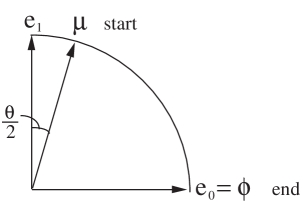
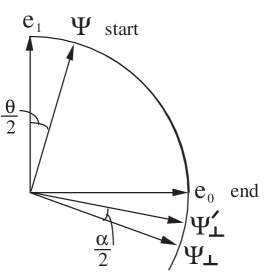
In understanding Grover’s algorithm, it is helpful to be aware of some simple properties of reflections on a plane. Suppose $\phi$ is a normalized ($\phi^{\dagger}\phi=1$) complex vector. Define the projection and reflection operators for $\phi$ by

$$\Pi_{\phi}=\phi\phi^{\dagger}\;,\;\;R_{\phi}=1-2\Pi_{\phi}\;.$$ (19)

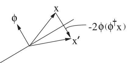
Note that $\Pi_{\phi}^{2}=\Pi_{\phi}$. Fig.1 shows that if $x^{\prime}=R_{\phi}x$, then $x^{\prime}$ is the reflection of $x$ with respect to the plane perpendicular to $\phi$. For example, $R_{\phi}\phi=-\phi$.

Figure 1: Reflection with respect to plane perpendicular to $\phi$.

Some simple properties of $R_{\phi}$ are as follows. $R_{\phi}=R_{\phi}^{\dagger}$ and $R_{\phi}R_{\phi}^{\dagger}=R_{\phi}^{2}=1$. Since reflections are unitary matrices, a product of reflections is also a unitary matrix.

Note that

$$(-1)^{\Pi_{\phi}} = e^{i\pi\Pi_{\phi}}=1+(e^{i\pi\Pi_{\phi}}-1)$$ (20a)

$$= 1+\Pi_{\phi}(e^{i\pi}-1)=1-2\Pi_{\phi}$$ (20b)

$$= R_{\phi}\;.$$ (20c)

(Eq.(20b) follows from the Taylor expansion of $e^{i\pi\Pi_{\phi}}$.)

If $e_{1},e_{2},\ldots,e_{n}$ is an orthonormal basis for a vector space, $\Pi_{i}=e_{i}e_{i}^{\dagger}$, and $R_{i}=1-2\Pi_{i}$, then the product of the $R_{i}$ in any order is $-1$. Indeed,

$$R_{1}R_{2}\ldots R_{n} = (1-2\Pi_{1})(1-2\Pi_{2})\ldots(1-2\Pi_{n})$$ (21a)

$$= 1-2(\Pi_{1}+\Pi_{2}+\ldots\Pi_{n})$$ (21b)

$$= -1\;.$$ (21c)

Another property of reflection operators which is useful for understanding Grover’s algorithm is the following. Let

$$e_{0}=\left(\begin{array}[]{c}1\\ 0\end{array}\right),\;\;e_{1}=\left(\begin{array}[]{c}0\\ 1\end{array}\right)\;.$$ (22)

Now suppose that $e^{\prime}_{1}$ is obtained by rotating $e_{1}$ clockwise by an angle $\theta/2$:

$$e^{\prime}_{1}=\left(\begin{array}[]{cc}\cos(\theta/2)&\sin(\theta/2)\\ -\sin(\theta/2)&\cos(\theta/2)\end{array}\right)e_{1}=\left(\begin{array}[]{c}\sin(\theta/2)\\ \cos(\theta/2)\end{array}\right)\;.$$ (23)

$e_{1}^{\prime}\approx e_{1}$ for small $\theta$. It is easy to check that the double reflection $-R_{e^{\prime}_{1}}R_{e_{0}}$ is equivalent to a rotation (also clockwise) by $\theta$:

$$-R_{e^{\prime}_{1}}R_{e_{0}}=\left(\begin{array}[]{cc}\cos\theta&\sin\theta\\ -\sin\theta&\cos\theta\end{array}\right)\;.$$ (24)

(That these two successive reflections equal a rotation was to be expected, since the reflections are orthogonal matrices and a product of orthogonal matrices is itself orthogonal.)

Above, we have considered plane reflections $R_{\phi}$ acting on a complex vector space, but our formulas still hold true when $R_{\phi}$ acts on a real instead of a complex vector space. In the case of real vector spaces, the Hermitian conjugate symbol $\dagger$ is replaced by the matrix transpose symbol $T$, and unitary matrices are replaced by orthogonal matrices.

3 Some Standard Algorithms

Next we will discuss several standard algorithms that are considered among the best that the quantum computation field has to offer at the present time. Later, we will try to generalize these standard algorithms.

3.1 Deutsch-Jozsa Algorithm

In this section we will discuss the D-J (Deutsch-Jozsa) algorithm[2]. We will do this first in terms of qubit circuits (the conventional approach), and then in terms of QB nets.

Figure 2: Qubit circuit for D-J’s algorithm.

Let $\vec{\kappa}=(\kappa_{0},\kappa_{1},\ldots,\kappa_{{N_{B}}-1})$ label ${N_{B}}$ “control” bits and let $\tau$ label a single “target” bit. Assume that $\tau$ and all the $\kappa_{i}$ are distinct. We will denote the state of these bits in the preferred basis (the eigenvectors of $\sigma_{z}$) by $|x\rangle_{\vec{\kappa}}|y\rangle_{\tau}$, where $x\in Bool^{N_{B}}$ and $y\in Bool$. Given a function $f:Bool^{N_{B}}\rightarrow Bool$, define the unitary operator $\Omega$ by

$$\Omega=\sigma_{x}(\tau)\hat{H}_{1}(\tau)\hat{H}_{1}(\vec{\kappa})\sigma_{x}^{f(\vec{{n}}(\vec{\kappa}))}(\tau)\hat{H}_{1}(\vec{\kappa})\hat{H}_{1}(\tau)\sigma_{x}(\tau)\;,$$ (25)

where $\vec{{n}}(\vec{\kappa})=({n}(\kappa_{0}),{n}(\kappa_{1}),\ldots,{n}(\kappa_{{N_{B}}-1}))$. The operation $\sigma_{x}^{f(\vec{{n}}(\vec{\kappa}))}(\tau)$, because it depends on $f$, is often called an “oracle” and each use of it is called a “query”. The right hand side of Eq.(25) may be represented by the circuit diagram shown in Fig.2. The D-J algorithm consists of applying $\Omega$ to an initial state $|0\rangle_{\vec{\kappa}}|0\rangle_{\tau}$ of bits $\vec{\kappa}$ and $\tau$, and then measuring the final state of these bits in the preferred basis.

Fig.2 and the right hand side of Eq.(25) are two equivalent ways of representing a particular SEO. There are infinitely many SEOs that yield $\Omega$. Fig.2 is just one of them. In fact, the original D-J paper[2] gave a different SEO for $\Omega$, one with two queries instead of one.

For $X\in Bool^{N_{B}},Y\in Bool$, let

$$|\psi_{0}\rangle=|X\rangle_{\vec{\kappa}}|Y\rangle_{\tau}\;,$$ (26)

and

$$|\psi_{i}\rangle=\Omega_{i}|\psi_{i-1}\rangle\;\;{\rm for}\;\;i=1,2,\ldots\;,$$ (27)

where

$$\Omega_{1}=\hat{H}_{1}(\vec{\kappa})\hat{H}_{1}(\tau)\sigma_{x}(\tau)\;,$$ (28)

$$\Omega_{2}=\sigma_{x}^{f(\vec{{n}}(\vec{\kappa}))}(\tau)\;,$$ (29)

and

$$\Omega_{3}=\Omega_{1}^{\dagger}\;.$$ (30)

Then it is easy to show using simple identities (such as $(H_{1})_{b,b^{\prime}}=(-1)^{bb^{\prime}}$, $\overline{0}=1$, $\overline{1}=0$, and $(-1)^{b}=(-1)^{-b}$ for $b,b^{\prime}\in Bool$) that

$$|\psi_{1}\rangle=\frac{1}{\sqrt{2^{{N_{B}}+1}}}\sum_{x,y}(-1)^{x\cdot X+y\overline{Y}}|x\rangle_{\vec{\kappa}}|y\rangle_{\tau}\;,$$ (31)

$$|\psi_{2}\rangle=\frac{1}{\sqrt{2^{{N_{B}}+1}}}\sum_{x,y}(-1)^{x\cdot X+y\overline{Y}}|x\rangle_{\vec{\kappa}}|y\oplus f(x)\rangle_{\tau}\;,$$ (32)

$$|\psi_{3}\rangle=\frac{1}{2^{{N_{B}}+1}}\sum_{x,y,X^{\prime},Y^{\prime}}(-1)^{x\cdot(X^{\prime}-X)+y(\overline{Y^{\prime}}-\overline{Y})+\overline{Y^{\prime}}f(x)}|X^{\prime}\rangle_{\vec{\kappa}}|Y^{\prime}\rangle_{\tau}\;.$$ (33)

Applying $\langle X^{\prime},Y^{\prime}|$ to the right hand side of Eq.(33) and using the identity Eq.(1) finally yields:

$$\langle X^{\prime},Y^{\prime}|\Omega|X,Y\rangle=\delta(Y^{\prime},Y)\frac{1}{2^{N_{B}}}\sum_{x\in Bool^{N_{B}}}(-1)^{x\cdot(X^{\prime}-X)+\overline{Y^{\prime}}f(x)}\;$$ (34)

for all $X^{\prime},X\in Bool^{N_{B}}$ and $Y^{\prime},Y\in Bool$. Thus, if the initial states of $\vec{\kappa}$ and $\tau$ are ${\underline{X}}=0$ and ${\underline{Y}}=0$, then the probability of obtaining ${\underline{X}}^{\prime}=X^{\prime}$ for the final state of $\vec{\kappa}$ is

$$P(X^{\prime}|{\underline{X}}={\underline{Y}}=0) = \sum_{Y^{\prime}}|\langle X^{\prime},Y^{\prime}|\Omega|X=0,Y=0\rangle|^{2}$$ (35)

$$= \frac{1}{4^{N_{B}}}|\sum_{x}(-1)^{x\cdot X^{\prime}+f(x)}|^{2}\;.$$

Let ${\cal F}_{bal}$, the set of “balanced” functions, be the set of all $f:Bool^{N_{B}}\rightarrow Bool$ such that $f$ maps exactly half of its domain to zero and half to one. Let ${\cal F}_{con}$, the set of “constant” functions, be the set of all $f:Bool^{N_{B}}\rightarrow Bool$ such that $f$ maps all its domain to zero or all of it to one. From Eq.(35), if $X^{\prime}=0$ and $f\in{\cal F}_{bal}\cup{\cal F}_{con}$, then

$$P({\underline{X}}^{\prime}=0|{\underline{X}}={\underline{Y}}=0)=\left\{\begin{array}[]{ll}1&{\rm if}\;\;f\in{\cal F}_{con}\\ 0&{\rm if}\;\;f\in{\cal F}_{bal}\end{array}\right.\;.$$ (36)

Now consider the QB net defined by Fig.3 and Table 3.1.

Figure 3: QB net for D-J’s algorithm.

nodes	states	amplitudes	comments
${\underline{X}}$	$X\in Bool^{N_{B}}$	$\delta(X,0)$
${\underline{Y}}$	$Y\in Bool$	$\delta(Y,0)$
${\underline{x}}$	$x\in Bool^{N_{B}}$	$(-1)^{x\cdot X}/{\sqrt{2^{N_{B}}}}$
${\underline{y}}$	$y\in Bool$	$(-1)^{y\overline{Y}}/{\sqrt{2}}$
${\underline{c}}$	$c=(c_{x},c_{y}),c_{x}\in Bool^{N_{B}},c_{y}\in Bool$	$\delta(c_{x},x)\delta(c_{y},y\oplus f(x))$
${\underline{x}}^{\prime}$	$x^{\prime}\in Bool^{N_{B}}$	$\delta(x^{\prime},c_{x})$
${\underline{y}}^{\prime}$	$y^{\prime}\in Bool$	$\delta(y^{\prime},c_{y})$
${\underline{X}}^{\prime}$	$X^{\prime}\in Bool^{N_{B}}$	$(-1)^{X^{\prime}\cdot x^{\prime}}/{\sqrt{2^{N_{B}}}}$
${\underline{Y}}^{\prime}$	$Y^{\prime}\in Bool$	$(-1)^{\overline{Y^{\prime}}y^{\prime}}/{\sqrt{2}}$

Table 1

For this net, the amplitude $A(x.)$ of net story $x.$ is the product of all the terms in the third column of Table 3.1. If ${\underline{X}}=0$ and ${\underline{Y}}=0$, then the probability of obtaining ${\underline{X}}^{\prime}=X^{\prime}$ is

$$P(X^{\prime}|{\underline{X}}={\underline{Y}}=0)=\frac{\sum_{Y^{\prime}}\left|\sum_{all/X^{\prime}Y^{\prime},X,Y}A(x.)|_{X=Y=0}\right|^{2}}{\sum_{X^{\prime}}num}\;,$$ (37)

where $A(x.)$ on the right hand side is evaluated at $X=Y=0$. Substituting the value of $A(x.)$ into Eq.(37) immediately yields Eq.(35).

Note that one can calculate the probability distribution Eq.(35) by means of a CB net instead of a QB net. One can do this with the CB net defined by the graph ${\underline{X}}^{\prime}\rightarrow{\underline{Y}}^{\prime}$, with:

nodes	states	probabilities	comments
${\underline{X}}^{\prime}$	$X^{\prime}\in Bool^{N_{B}}$	$P_{{\underline{X}}^{\prime}}(X^{\prime})$
${\underline{Y}}^{\prime}$	$Y^{\prime}\in Bool$	$P_{{\underline{Y}}^{\prime}|{\underline{X}}^{\prime}}(Y^{\prime}|X^{\prime})$

Table 2

where $P_{{\underline{X}}^{\prime}}$ and $P_{{\underline{Y}}^{\prime}|{\underline{X}}^{\prime}}$ are calculated from

$$P_{{\underline{X}}^{\prime},{\underline{Y}}^{\prime}}(X^{\prime},Y^{\prime})=|\langle X^{\prime},Y^{\prime}|\Omega|X=0,Y=0\rangle|^{2}\;.$$ (38)

We will say that the CB net defined by the graph ${\underline{X}}^{\prime}\rightarrow{\underline{Y}}^{\prime}$ and Table 3.1 is “q-embedded” in the QB net defined by Fig.3 and Table 3.1. In subsequent sections, we will say much more about q-embedding of CB nets.

3.2 Simon’s Algorithm

In this section we will discuss Simon’s algorithm[3]. We will do this first in terms of qubit circuits (the conventional approach), and then in terms of QB nets.

Figure 4: Qubit circuit for Simon’s algorithm.

Simon’s algorithm uses ${N_{B}}$ “control” bits, just like the D-J algorithm. However, it uses ${N_{B}}$ target bits whereas the D-J algorithm uses only one. Simon’s algorithm deals with a vector-valued function $f:Bool^{N_{B}}\rightarrow Bool^{N_{B}}$, whereas D-J’s algorithm deals with a scalar-valued function $f:Bool^{N_{B}}\rightarrow Bool$. Let $\vec{\kappa}=(\kappa_{0},\kappa_{1},\ldots,\kappa_{{N_{B}}-1})$ label ${N_{B}}$ “control” bits and let $\vec{\tau}=(\tau_{0},\tau_{1},\ldots,\tau_{{N_{B}}-1})$ label ${N_{B}}$ “target” bits. Assume all $\tau_{i}$ and $\kappa_{i}$ are distinct. We will denote the state of these bits in the preferred basis (the eigenvectors of $\sigma_{z}$) by $|x\rangle_{\vec{\kappa}}|y\rangle_{\vec{\tau}}$, where $x\in Bool^{N_{B}}$ and $y\in Bool^{N_{B}}$. Given a function $f=(f_{0},f_{1},\ldots,f_{{N_{B}}-1})$ where $f_{i}:Bool^{N_{B}}\rightarrow Bool$, define the unitary operator $\Omega$ by

$$\Omega=\hat{H}_{1}(\vec{\kappa})\left[\prod_{i=0}^{{N_{B}}-1}\sigma_{x}^{f_{i}(\vec{{n}}(\vec{\kappa}))}(\tau_{i})\right]\hat{H}_{1}(\vec{\kappa})\;.$$ (39)

The operator $\Omega$ for Simon’s algorithm is analogous to the $\Omega$ defined by Eq.(25) for the D-J algorithm. The right hand side of Eq.(39) may be represented by the circuit diagram of Fig.4. Simon’s algorithm consists of applying $\Omega$ given by Eq.(39) to an initial state $|0\rangle_{\vec{\kappa}}|0\rangle_{\vec{\tau}}$ of bits $\vec{\kappa}$ and $\vec{\tau}$, and then measuring the final state of these bits in the preferred basis. One performs this routine several times. The measurement outcomes allow one to determine the period of the function $f$ if $f$ is of a special periodic type that will be specified later.

Using the same techniques that we used to evaluate the matrix elements of $\Omega$ for the D-J algorithm, one finds

$$\langle X^{\prime},Y^{\prime}|\Omega|X,Y\rangle=\frac{1}{2^{N_{B}}}\sum_{x\in Bool^{N_{B}}}(-1)^{x\cdot(X^{\prime}-X)}\delta(Y^{\prime},Y\oplus f(x))\;,$$ (40)

for all $X^{\prime},Y^{\prime},X,Y\in Bool^{N_{B}}$. If the initial states of $\vec{\kappa}$ and $\vec{\tau}$ are ${\underline{X}}=0$ and ${\underline{Y}}=0$, then the probability of obtaining ${\underline{X}}^{\prime}=X^{\prime}$ for the final state of $\vec{\kappa}$ is

$$P(X^{\prime}|{\underline{X}}={\underline{Y}}=0) = \sum_{Y^{\prime}}|\langle X^{\prime},Y^{\prime}|\Omega|X=0,Y=0\rangle|^{2}$$ (41)

$$= \frac{1}{4^{N_{B}}}\sum_{Y^{\prime}}|\sum_{x}(-1)^{x\cdot X^{\prime}}\delta(Y^{\prime},f(x))|^{2}\;.$$

Now suppose ${\cal F}_{S}$ is the set of those functions $f:Bool^{N_{B}}\rightarrow Bool^{N_{B}}$ such that $f$ is 2 to 1 (i.e., $f$ maps exactly two domain points into each image point) and has a “period” $\Delta$. By a period $\Delta$, we mean a non-zero element of $Bool^{N_{B}}$ such that $f(x)=f(x\oplus\Delta)$ for all $x\in Bool^{N_{B}}$. For any $f\in{\cal F}_{S}$ and any $y\in Bool^{N_{B}}$, there exist exactly two elements of $Bool^{N_{B}}$, call them $x_{1}$ and $x_{2}$, such that $x_{1}=x_{2}\oplus\Delta$ and $f(x_{1})=f(x_{2})=y$. Call $f^{-1}_{p}(y)$ one of these $x$ values, and call $f^{-1}_{p}(y)\oplus\Delta$ the other. (The $p$ subscript stands for “principal part”, in analogy with Complex Analysis.) If $f\in{\cal F}_{S}$, and $I(f)$ is the image of $f$, then

$$\delta(Y^{\prime},f(x))=\left\{\begin{array}[]{ll}\delta(f^{-1}_{p}(Y^{\prime}),x)+\delta(f^{-1}_{p}(Y^{\prime})\oplus\Delta,x),&{\rm if}\;\;Y^{\prime}\in I(f)\\ 0&{\rm otherwise}\end{array}\right.\;.$$ (42)

Substituting this expression for $\delta(Y^{\prime},f(x))$ into Eq.(41) and using Eq.(1) yields

$$P(X^{\prime}|{\underline{X}}={\underline{Y}}=0)=\frac{1}{2^{{N_{B}}-1}}\delta(X^{\prime}\cdot\Delta,0)\;.$$ (43)

To calculate the period $\Delta$ of $f$, run the experiment $\nu$ times, measuring $X^{\prime}$ each time. Let $X^{\prime}(i)$ represent the $i$th measurement outcome. Then, for sufficiently large $\nu$, one can find $\Delta$ by solving the equations $X^{\prime}(1)\cdot\Delta=0$, $X^{\prime}(2)\cdot\Delta=0$, … , $X^{\prime}(\nu)\cdot\Delta=0$.

Now consider the QB net defined by Fig.5 and Table 3.2.

Figure 5: QB net for Simon’s algorithm.

nodes	states	amplitudes	comments
${\underline{X}}$	$X\in Bool^{N_{B}}$	$\delta(X,0)$
${\underline{Y}}$	$Y\in Bool^{N_{B}}$	$\delta(Y,0)$
${\underline{x}}$	$x\in Bool^{N_{B}}$	$(-1)^{x\cdot X}/{\sqrt{2^{N_{B}}}}$
${\underline{c}}$	$c=(c_{x},c_{y});c_{x},c_{y}\in Bool^{N_{B}}$	$\delta(c_{x},x)\delta(c_{y},Y\oplus f(x))$
${\underline{x}}^{\prime}$	$x^{\prime}\in Bool^{N_{B}}$	$\delta(x^{\prime},c_{x})$
${\underline{X}}^{\prime}$	$X^{\prime}\in Bool^{N_{B}}$	$(-1)^{X^{\prime}\cdot x^{\prime}}/{\sqrt{2^{N_{B}}}}$
${\underline{Y}}^{\prime}$	$Y^{\prime}\in Bool^{N_{B}}$	$\delta(Y^{\prime},c_{y})$

Table 3

For this net, the amplitude $A(x.)$ of net story $x.$ is the product of all the terms in the third column of Table 3.2. If ${\underline{X}}=0$ and ${\underline{Y}}=0$, then the probability of obtaining ${\underline{X}}^{\prime}=X^{\prime}$ is

$$P(X^{\prime}|{\underline{X}}={\underline{Y}}=0)=\frac{\sum_{Y^{\prime}}\left|\sum_{all/X^{\prime}Y^{\prime},X,Y}A(x.)|_{X=Y=0}\right|^{2}}{\sum_{X^{\prime}}num}\;,$$ (44)

where $A(x.)$ on the right hand side is evaluated at $X=Y=0$. Substituting the value of $A(x.)$ into Eq.(44) immediately yields Eq.(41).

It is possible to calculate the probability distribution Eq.(41) by means of a CB net instead of a QB net. One can do this with the CB net defined by the graph ${\underline{X}}^{\prime}\rightarrow{\underline{Y}}^{\prime}$, with:

nodes	states	probabilities	comments
${\underline{X}}^{\prime}$	$X^{\prime}\in Bool^{N_{B}}$	$P_{{\underline{X}}^{\prime}}(X^{\prime})$
${\underline{Y}}^{\prime}$	$Y^{\prime}\in Bool^{N_{B}}$	$P_{{\underline{Y}}^{\prime}|{\underline{X}}^{\prime}}(Y^{\prime}|X^{\prime})$

Table 4

where $P_{{\underline{X}}^{\prime}}$ and $P_{{\underline{Y}}^{\prime}|{\underline{X}}^{\prime}}$ are calculated from

$$P_{{\underline{X}}^{\prime},{\underline{Y}}^{\prime}}(X^{\prime},Y^{\prime})=|\langle X^{\prime},Y^{\prime}|\Omega|X=0,Y=0\rangle|^{2}\;.$$ (45)

We will say that the CB net defined by the graph ${\underline{X}}^{\prime}\rightarrow{\underline{Y}}^{\prime}$ and Table 3.2 is “q-embedded” in the QB net defined by Fig.5 and Table 3.2.

3.3 Bernstein-Vazirani Algorithm

In this section we will discuss the B-V (Bernstein-Vazirani) algorithm[4].

To understand the B-V algorithm, it is helpful to first establish the following simple single qubit identities. First note that the single qubit Hadamard matrix rotates the $Z$-direction number operator into the $X$-direction number operator:

$$\hat{H}_{1}{n}_{z}\hat{H}_{1}=\frac{1}{2}\left(\begin{array}[]{cc}1&-1\\ -1&1\end{array}\right)={n}_{x}\;.$$ (46)

Thus,

$$\sigma_{x}^{b}=[(-1)^{{n}_{x}}]^{b}=(-1)^{b{n}_{x}}=\hat{H}_{1}(-1)^{b{n}_{z}}\hat{H}_{1}\;.$$ (47)

Next note that $\sigma_{x}$ exchanges the components of any vector it acts on:

$$\sigma_{x}\left(\begin{array}[]{c}\alpha\\ \beta\end{array}\right)=\left(\begin{array}[]{c}\beta\\ \alpha\end{array}\right)\;,$$ (48)

for any complex numbers $\alpha,\beta$. In particular, if $b\in Bool$, then

$$\sigma_{x}^{b}|0\rangle=|b\rangle\;.$$ (49)

Now we are ready to discuss the B-V algorithm. Let $\vec{\kappa}=(\kappa_{0},\kappa_{1},\ldots,\kappa_{{N_{B}}-1})$ label ${N_{B}}$ “control” bits and let $\tau$ label a single “target” bit. Assume that $\tau$ and all the $\kappa_{i}$ are distinct. We will denote the state of these bits in the preferred basis (the eigenvectors of $\sigma_{z}$) by $|x\rangle_{\vec{\kappa}}|y\rangle_{\tau}$, where $x\in Bool^{N_{B}}$ and $y\in Bool$. For $\vec{b}\in Bool^{N_{B}}$, define the unitary operator

$$\omega_{\vec{b}}=\prod_{i=0}^{{N_{B}}-1}\sigma_{x}(\kappa_{i})^{b_{i}}\;.$$ (50)

The B-V algorithm is simply the following multi-qubit generalization of Eq.(49)

$$\omega_{\vec{b}}|0\rangle_{\vec{\kappa}}=|\vec{b}\rangle_{\vec{\kappa}}\;.$$ (51)

That’s all there is to B-V!

Eq.(51) can be represented by a qubit circuit consisting of a single wire for $\vec{\kappa}$, with a single node representing $\omega_{\vec{b}}$. Eq.(51) can also be represented by a QB net defined by the graph ${\underline{X}}\rightarrow{\underline{X}}^{\prime}$, with

nodes	states	amplitudes	comments
${\underline{X}}$	$X=(X_{0},X_{1},X_{{N_{B}}-1})\in Bool^{N_{B}}$	$\delta(X,0)$
${\underline{X}}^{\prime}$	$X^{\prime}=(X^{\prime}_{0},X^{\prime}_{1},X^{\prime}_{{N_{B}}-1})\in Bool^{N_{B}}$	$\prod_{i=0}^{{N_{B}}-1}\delta^{b_{i}}(X^{\prime}_{i},\overline{X_{i}})$

Table 5

We should mention that it is common in the literature to dress up and obfuscate Eq.(50) as follows. By virtue of Eq.(47), one can re-express $\omega_{\vec{b}}$ as

$$\omega_{\vec{b}}=\prod_{i=0}^{{N_{B}}-1}\sigma_{x}(\kappa_{i})^{b_{i}}=\hat{H}_{1}(\vec{\kappa})(-1)^{\sum_{i=0}^{{N_{B}}-1}b_{i}{n}_{z}(\kappa_{i})}\hat{H}_{1}(\vec{\kappa})\;.$$ (52)

Some workers ascend to an even higher peak of obfuscation by adding a totally unnecessary target qubit. They define an operator, call it $\Omega_{\vec{b}}$, obtained by replacing the $(-1)$ in Eq.(52) by the operator $\sigma_{x}(\tau)$ acting on a target qubit $\tau$:

$$\Omega_{\vec{b}}=\hat{H}_{1}(\vec{\kappa})[\sigma_{x}(\tau)]^{\sum_{i=0}^{{N_{B}}-1}b_{i}{n}_{z}(\kappa_{i})}\hat{H}_{1}(\vec{\kappa})\;.$$ (53)

At the beginning of the experiment, they put the target qubit in a state which is an eigenvector of $\sigma_{x}(\tau)$ with eigenvalue $-1$. Thus, the obfuscated version of the B-V algorithm with a target qubit can be summarized by

$$\Omega_{\vec{b}}|-_{x}\rangle_{\tau}|0\rangle_{\vec{\kappa}}=\omega_{\vec{b}}|-_{x}\rangle_{\tau}|0\rangle_{\vec{\kappa}}=|-_{x}\rangle_{\tau}|\vec{b}\rangle_{\vec{\kappa}}\;.$$ (54)

We emphasize that for the B-V algorithm, the target qubit is a totally unnecessary affectation.

So far we have given an unconventional presentation of the B-V algorithm. For completeness, we now give a conventional one. Define

$$|\psi_{0}\rangle=|0\rangle_{\vec{\kappa}}|-_{x}\rangle_{\tau}\;,$$ (55)

and

$$|\psi_{i}\rangle=\Omega_{i}|\psi_{i-1}\rangle\;\;{\rm for}\;\;i=1,2,\ldots\;,$$ (56)

where

$$\Omega_{1}=\hat{H}_{1}(\vec{\kappa})\;,$$ (57)

$$\Omega_{2}=[\sigma_{x}(\tau)]^{\sum_{i=0}^{{N_{B}}-1}b_{i}{n}_{z}(\kappa_{i})}\;,$$ (58)

and

$$\Omega_{3}=\Omega_{1}\;.$$ (59)

It follows that

$$|\psi_{1}\rangle=\frac{1}{\sqrt{2^{N_{B}}}}\sum_{\vec{x}\in Bool^{N_{B}}}|\vec{x}\rangle_{\vec{\kappa}}|-_{x}\rangle_{\tau}\;,$$ (60)

$$|\psi_{2}\rangle=\frac{1}{\sqrt{2^{N_{B}}}}\sum_{\vec{x}}(-1)^{\vec{b}\cdot\vec{x}}|\vec{x}\rangle_{\vec{\kappa}}|-_{x}\rangle_{\tau}\;,$$ (61)

and

$$|\psi_{3}\rangle = \frac{1}{\sqrt{2^{N_{B}}}}\sum_{\vec{x}}(-1)^{\vec{b}\cdot\vec{x}}\frac{1}{\sqrt{2^{N_{B}}}}\sum_{\vec{y}}(-1)^{\vec{y}\cdot\vec{x}}|\vec{y}\rangle_{\vec{\kappa}}|-_{x}\rangle_{\tau}$$ (62a)

$$= \frac{1}{2^{N_{B}}}\sum_{\vec{x},\vec{y}}(-1)^{(\vec{b}-\vec{y})\cdot\vec{x}}|\vec{y}\rangle_{\vec{\kappa}}|-_{x}\rangle_{\tau}$$ (62b)

$$= |\vec{b}\rangle_{\vec{\kappa}}|-_{x}\rangle_{\tau}\;.$$ (62c)

To go from step (b) to step (c) of Eq.(62), we used the orthogonality property given by Eq.(1).

3.4 Grover’s Algorithm

In this section we will discuss Grover’s algorithm [5].

Let $\vec{\kappa}=(\kappa_{0},\kappa_{1},\ldots,\kappa_{{N_{B}}-1})$ label ${N_{B}}$ bits. Assume all $\kappa_{i}$ are distinct. We begin by defining the following ${N_{S}}$-dimensional column vectors:

$$|\mu\rangle_{\vec{\kappa}}=\mu=\mu_{N_{S}}=\frac{1}{\sqrt{{N_{S}}}}[1,1,1,1\ldots,1]^{T}=\frac{1}{\sqrt{{N_{S}}}}H_{N_{B}}[1,0,0,0,\ldots,0]^{T}\;,$$ (63)

$$|\phi\rangle_{\vec{\kappa}}=\phi=[0,\ldots,0,0,1,0,0,\ldots,0]^{T}\;.$$ (64)

All components of $\phi$ are zero except for one predetermined component, located at position $j_{targ}\in Z_{0,{N_{S}}-1}$, which equals one. We will refer to $j_{targ}$ as the target state (not to be confused with a target qubit). Note that we chose a special basis (or, equivalently, a special matrix representation) from the start. Note that $\langle\phi|\mu\rangle=\frac{1}{\sqrt{{N_{S}}}}$, so $\mu$ and $\phi$ are nearly orthogonal for large ${N_{S}}$. It is also convenient to define the component-wise negation of $\phi$:

$$|\phi^{not}\rangle_{\vec{\kappa}}=\phi^{not}=[1,\ldots,1,1,0,1,1,\ldots,1]^{T}\;.$$ (65)

Note that $\phi^{not}$ is not normalized.

Define projection and reflection operators for $\mu$ and $\phi$:

$$\Pi_{\mu}=|\mu\rangle\langle\mu|\;,\;\;R_{\mu}=1-2\Pi_{\mu}=(-1)^{\Pi_{\mu}}\;,$$ (66)

and

$$\Pi_{\phi}=|\phi\rangle\langle\phi|\;,\;\;R_{\phi}=1-2\Pi_{\phi}=(-1)^{\Pi_{\phi}}\;.$$ (67)

Grover’s algorithm can be summarized by the following equation[10][11]:

$$(-R_{\mu}R_{\phi})^{r}\mu\approx\phi\;,$$ (68)

for some integer $r$ to be determined, where “$\approx$” means approximation at large ${N_{S}}$. Thus, starting with an ${N_{B}}$ qubit system in a state $\mu$, one applies the operator $(-R_{\mu}R_{\phi})$ consecutively $r$ times, so that the ${N_{B}}$ qubit system ends in a state as close to $\phi$ as possible. Measuring state $\phi$ in the special basis yields the target state $j_{targ}$.

Eq.(68) can be represented by a qubit circuit consisting of a single wire for $\vec{\kappa}$, with $r$ nodes, each representing $-R_{\mu}R_{\phi}$. Eq.(68) can also be represented by a QB net defined by a Markov chain graph ${\underline{X}}_{0}\rightarrow{\underline{X}}_{1}\rightarrow{\underline{X}}_{2}\rightarrow\ldots\rightarrow{\underline{X}}_{r-1}$, with

nodes	states	amplitudes	comments
${\underline{X}}_{0}$	$X_{0}\in Bool^{N_{B}}$	$\delta(X_{0},0)$
${\underline{X}}_{i}$ for $i\in Z_{1,r-1}$	$X_{i}\in Bool^{N_{B}}$	$\langle X_{i}|(-R_{\mu}R_{\phi})|X_{i-1}\rangle$

Table 6

To find the optimum number $r$ of iterations, one can proceed as follows.

First, notice that Eq.(68) describes a process which is entirely confined to the vector subspace spanned by $\mu$ and $\phi$. Since $\mu$ and $\phi$ are not orthogonal, it is convenient to define an orthonormal basis $e_{0},e_{1}$ for the space $span(\mu,\phi)$. Let

$$e_{0}=\phi\;,\;\;e_{1}=\frac{\phi^{not}}{\sqrt{{N_{S}}-1}}\;.$$ (69)

Then

$$\mu=\frac{1}{\sqrt{{N_{S}}}}(e_{0}+\sqrt{{N_{S}}-1}\;e_{1})\;.$$ (70)

Fig.6 portrays various vectors that arise in explaining Grover’s algorithm.

Figure 6: Various vectors relevant to Grover’s Algorithm.

Since we plan to stay within the two dimensional vector space with orthonormal basis $e_{0},e_{1}$, it is convenient to switch matrix representations. Within $span(e_{0},e_{1})$, $e_{0},e_{1}$ can be represented more simply by:

$$e_{0}=\left(\begin{array}[]{c}1\\ 0\end{array}\right)\;,\;\;e_{1}=\left(\begin{array}[]{c}0\\ 1\end{array}\right)\;.$$ (71)

If $e_{0},e_{1}$ are represented in this way, then

$$\phi=\left(\begin{array}[]{c}1\\ 0\end{array}\right)\;,\;\;\mu=\frac{1}{\sqrt{{N_{S}}}}\left(\begin{array}[]{c}1\\ \sqrt{{N_{S}}-1}\end{array}\right)\;,$$ (72)

and

$$-R_{\mu}R_{\phi}=\frac{1}{{N_{S}}}\left(\begin{array}[]{cc}{N_{S}}-2&2\sqrt{{N_{S}}-1}\\ -2\sqrt{{N_{S}}-1}&{N_{S}}-2\end{array}\right)\;.$$ (73)

Thus,

$$-R_{\mu}R_{\phi}=\left(\begin{array}[]{cc}\cos\theta&\sin\theta\\ -\sin\theta&\cos\theta\end{array}\right)\;,$$ (74)

where

$$\sin\theta=\frac{2\sqrt{{N_{S}}-1}}{{N_{S}}}\approx\frac{2}{\sqrt{{N_{S}}}}\;.$$ (75)

Eq.(74) is just Eq.(24) with $e^{\prime}_{1}=\mu$ and $e_{0}=\phi$. It follows that

$$(-R_{\mu}R_{\phi})^{r}=\left(\begin{array}[]{cc}\cos(r\theta)&\sin(r\theta)\\ -\sin(r\theta)&\cos(r\theta)\end{array}\right)\;,$$ (76)

and

$$(-R_{\mu}R_{\phi})^{r}\mu = \left(\begin{array}[]{cc}\cos(r\theta)&\sin(r\theta)\\ -\sin(r\theta)&\cos(r\theta)\end{array}\right)\frac{1}{\sqrt{{N_{S}}}}\left(\begin{array}[]{c}1\\ \sqrt{{N_{S}}-1}\end{array}\right)$$ (81)

$$\approx \left(\begin{array}[]{c}\sin(r\theta)\\ \cos(r\theta)\end{array}\right)\;.$$ (84)

We want the final state of the system to be parallel or anti-parallel to $e_{0}=\phi$ ; therefore, we want

$$\left(\begin{array}[]{c}\sin(r\theta)\\ \cos(r\theta)\end{array}\right)\approx\left(\begin{array}[]{c}\pm 1\\ 0\end{array}\right)\;.$$ (85)

This will occur if

$$r\theta\approx\frac{\pi}{2}(1+2k)\;\;,\;\;r\approx\frac{\pi}{4}(1+2k)\sqrt{{N_{S}}}$$ (86)

for some integer $k$.

Note that, in Grover’s algorithm, the number of “queries” (calls to a unitary matrix that depends on $\phi$) is far from unique. To illustrate this, let $Q$ be a permutation matrix that satisfies

$$Q\phi=|0\rangle=[1,0,0,\ldots,0]^{T}\;.$$ (87)

Since all the components of $\mu$ are equal, $Q\mu=\mu$. Thus

$$(-R_{\mu}R_{\phi})^{r}\mu=Q^{T}(-R_{\mu}R_{|0\rangle})^{r}Q\mu=Q^{T}(-R_{\mu}R_{|0\rangle})^{r}\mu\;.$$ (88)

Hence, it is possible to accomplish the full Grover transformation of $\mu$ with only a single query $Q^{T}$.

Since $\left(\begin{array}[]{cc}0&1\\ -1&0\end{array}\right)\left(\begin{array}[]{c}a\\ b\end{array}\right)=\left(\begin{array}[]{c}b\\ -a\end{array}\right)$, the matrix $\left(\begin{array}[]{cc}0&1\\ -1&0\end{array}\right)$ is just a clockwise rotation by $\pi/2$. Let

$$U_{Grov} = \left(\begin{array}[]{cc}0&1\\ -1&0\end{array}\right)$$

$$= -e_{1}e_{0}^{T}+e_{0}e_{1}^{T}$$

$$= \frac{1}{\sqrt{{N_{S}}-1}}[-\phi^{not}\phi^{T}+\phi(\phi^{not})^{T}]\;.$$ (92)

Note that

$$U_{Grov}\mu = \frac{1}{\sqrt{{N_{S}}-1}}\left(-\phi^{not}[\phi^{T}\mu]+\phi[(\phi^{not})^{T}\mu]\right)$$ (93)

$$= \frac{1}{\sqrt{{N_{S}}({N_{S}}-1)}}[-\phi^{not}+({N_{S}}-1)\phi]\;.$$

From the point of view of quantum compiling, what Grover found is that the $\pi/2$ rotation $U_{Grov}$ is (approximately) equal to the $r$-fold product of $-R_{\mu}R_{\phi}$, where $-R_{\mu}R_{\phi}$ can be shown to have a SEO of low (polynomial in ${N_{B}}$) complexity.

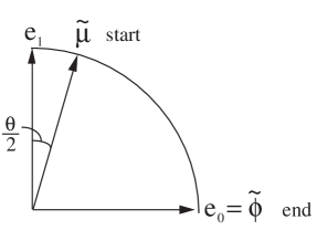
Grover’s algorithm has been modified in various, minor ways since it was first published. For example, Brassard et al. pointed out in Ref.[12] that the vector $\mu$ need not be the vector whose components are all equal. Other vectors $\mu$ will do just as well. Another modification of Grover’s algorithm due to Younes-Miller[13] adds an extra qubit to the original ${N_{B}}$ qubits. Next we will discuss the Younes-Miller modification of Grover’s algorithm, because it resembles a modification of Grover’s algorithm that we will use in a future section.

Let $\vec{\kappa}=(\kappa_{0},\kappa_{1},\ldots,\kappa_{{N_{B}}-1})$ label ${N_{B}}$ bits. Let $\tau$ label a single bit. Assume $\tau$ and all the $\kappa_{i}$ are distinct. Let $\mu$ and $\phi$ denote the same ${N_{S}}$ dimensional column vectors that we used in discussing the original Grover algorithm. In addition, define the following $2{N_{S}}$ dimensional column vectors:

$$|{\tilde{\mu}}\rangle=|+_{z}\rangle_{\tau}|\mu\rangle_{\vec{\kappa}}=\left(\begin{array}[]{c}1\\ 0\end{array}\right)\otimes\mu_{N_{S}}=\left(\begin{array}[]{c}\mu_{N_{S}}\\ 0\end{array}\right)\;,$$ (94)

$$|{\tilde{\phi}}\rangle=|-_{x}\rangle_{\tau}|\phi\rangle_{\vec{\kappa}}=\frac{1}{\sqrt{2}}\left(\begin{array}[]{c}1\\ -1\end{array}\right)\otimes\phi=\frac{1}{\sqrt{2}}\left(\begin{array}[]{c}\phi\\ -\phi\end{array}\right)\;.$$ (95)

Note that $\langle{\tilde{\phi}}|{\tilde{\mu}}\rangle=\frac{1}{\sqrt{2{N_{S}}}}$, so ${\tilde{\phi}}$ and ${\tilde{\mu}}$ are nearly orthogonal for large ${N_{S}}$. Define projection and reflection operators for ${\tilde{\phi}}$ in the usual way:

$$\Pi_{{\tilde{\phi}}}=|{\tilde{\phi}}\rangle\langle{\tilde{\phi}}|\;,\;R_{{\tilde{\phi}}}=1-2\Pi_{{\tilde{\phi}}}=1-2\Pi_{|\phi\rangle_{\vec{\kappa}}}\Pi_{|-_{x}\rangle_{\tau}}\;.$$ (96)

$R_{{\tilde{\phi}}}$ can be re-expressed as

$$R_{{\tilde{\phi}}} = 1+\Pi_{|\phi\rangle_{\vec{\kappa}}}(\sigma_{x}(\tau)-1)=\exp[{\Pi_{|\phi\rangle_{\vec{\kappa}}}\ln\sigma_{x}(\tau)}]=$$ (97)

$$= [\sigma_{x}(\tau)]^{\Pi_{|\phi\rangle_{\vec{\kappa}}}}\;.$$

Define projection and reflection operators for ${\tilde{\mu}}$ in the usual way:

$$\Pi_{{\tilde{\mu}}}=|{\tilde{\mu}}\rangle\langle{\tilde{\mu}}|\;,\;R_{{\tilde{\mu}}}=1-2\Pi_{{\tilde{\mu}}}=1-2\Pi_{|\mu\rangle_{\vec{\kappa}}}\Pi_{|+_{z}\rangle_{\tau}}\;.$$ (98)

$R_{{\tilde{\mu}}}$ can be re-expressed as

$$R_{{\tilde{\mu}}}=\hat{H}_{1}(\vec{\kappa})\left(1-2\Pi_{|0\rangle_{\vec{\kappa}}}\Pi_{|0\rangle_{\tau}}\right)\hat{H}_{1}(\vec{\kappa})\;.$$ (99)

In analogy with the original Grover’s algorithm, the Younes-Miller version can be summarized by

$$(-R_{{\tilde{\mu}}}R_{{\tilde{\phi}}})^{r}|{\tilde{\mu}}\rangle\approx|{\tilde{\phi}}\rangle\;,$$ (100)

for some integer $r$ to be determined, where “$\approx$” means approximation at large ${N_{S}}$. Thus, starting with an ${N_{B}}+1$ qubit system in a state ${\tilde{\mu}}$, one applies the operator $(-R_{\mu}R_{\phi})$ consecutively $r$ times, so that the final state of the ${N_{B}}+1$ qubit system ends in a state as close to ${\tilde{\phi}}$ as possible. Measuring state ${\tilde{\phi}}$ in the special basis yields the target state $j_{targ}$.

To find the optimum number $r$ of iterations, one can proceed as follows.

First, notice that Eq.(100) describes a process which is entirely confined to the vector subspace spanned by ${\tilde{\mu}}$ and ${\tilde{\phi}}$. Since ${\tilde{\mu}}$ and ${\tilde{\phi}}$ are not orthogonal, it is convenient to define an orthonormal basis $e_{0},e_{1}$ for the space $span({\tilde{\mu}},{\tilde{\phi}})$. Let

$$e_{0}={\tilde{\phi}}=\frac{1}{\sqrt{2}}\left(\begin{array}[]{c}\phi\\ -\phi\end{array}\right)\;,$$ (101)

and

$$e_{1}=\frac{1}{K}[{\tilde{\mu}}-({\tilde{\mu}}\cdot e_{0})e_{0}]\;,$$ (102)

where $K$ is chosen so that $e_{1}^{2}=1$. It is easy to show that

$$K=|{\tilde{\mu}}-({\tilde{\mu}}\cdot e_{0})e_{0}|=\sqrt{\frac{{N_{S}}-\frac{1}{2}}{{N_{S}}}}\;.$$ (103)

Thus,

$$e_{1}=\frac{1}{\sqrt{{N_{S}}-\frac{1}{2}}}\left(\begin{array}[]{c}\phi^{not}+\frac{\phi}{2}\\ \frac{\phi}{2}\end{array}\right)\;.$$ (104)

Furthermore,

$${\tilde{\mu}}=\frac{1}{\sqrt{2{N_{S}}}}[e_{0}+\sqrt{2{N_{S}}-1}\;e_{1}]\;.$$ (105)

Fig.7 portrays various vectors that arise in explaining Younes’ version of Grover’s algorithm.

Figure 7: Various vectors relevant to Younes’ version of Grover’s Algorithm.

Since we plan to stay within the two dimensional vector space with orthonormal basis $e_{0},e_{1}$, it is convenient to switch matrix representations. Within $span(e_{0},e_{1})$, $e_{0},e_{1}$ can be represented more simply by:

$$e_{0}=\left(\begin{array}[]{c}1\\ 0\end{array}\right)\;,\;\;e_{1}=\left(\begin{array}[]{c}0\\ 1\end{array}\right)\;.$$ (106)

If $e_{0},e_{1}$ are represented this way, then

$${\tilde{\phi}}=\left(\begin{array}[]{c}1\\ 0\end{array}\right)\;,\;\;{\tilde{\mu}}=\frac{1}{\sqrt{2{N_{S}}}}\left(\begin{array}[]{c}1\\ \sqrt{2{N_{S}}-1}\end{array}\right)\;,$$ (107)

and

$$-R_{{\tilde{\mu}}}R_{\tilde{\phi}}=\frac{1}{{N_{S}}}\left(\begin{array}[]{cc}{N_{S}}-1&\sqrt{2{N_{S}}-1}\\ -\sqrt{2{N_{S}}-1}&{N_{S}}-1\end{array}\right)\;.$$ (108)

Thus,

$$-R_{{\tilde{\mu}}}R_{\tilde{\phi}}=\left(\begin{array}[]{cc}\cos\theta&\sin\theta\\ -\sin\theta&\cos\theta\end{array}\right)\;,$$ (109)

where

$$\sin\theta=\frac{\sqrt{2{N_{S}}-1}}{{N_{S}}}\approx\sqrt{\frac{2}{{N_{S}}}}\;.$$ (110)

A comparison of Eq.(72) (for the original Grover’s algorithm) and Eq.(107) (for Younes’s version of Grover’s algorithm) reveals that for the purpose of finding the optimal number $r$ of iterations, Younes’ algorithm is the same as Grover’s algorithm if one replaces ${N_{S}}$ in Grover’s algorithm by $2{N_{S}}$. This comes from the fact that Younes’ algorithm uses ${N_{B}}+1$ bits whereas Grover’s uses ${N_{B}}$.

4 Generalization of Standard Algorithms,
a list of Desiderata

So far we have analyzed several standard quantum computing algorithms, namely those attributed to Deutsch-Jozsa, Bernstein-Vazirani, Simon and Grover. (Two other standard algorithm’s that we didn’t analyze are Shor’s algorithm[14] and the algorithm for Teleportation[15].) In this section, we will try to point out those features of the standard algorithms that would be, in our opinion, fruitful to generalize. Bear in mind that generalizations are seldom unique, but some are more natural, fruitful and far-reaching than others.

(a) Allow more complicated graph topologies

The standard algorithms discussed here can all be represented by QB nets with trivial topologies such as 2 body scattering graphs or Markov chains. However, other important quantum algorithms, such as the one for Teleportation[15], can be represented by QB nets with more complicated graph topologies (e.g., with loops).

(b) Estimate more general probability distributions

The goal of most standard algorithms is to estimate a deterministic probability distribution. However, estimating non-deterministic ones is also very useful. Such estimates are useful in, for example, applications of Decision Theory and Artificial Intelligence, where inferences are made based on uncertain knowledge.

(c) Allow multiple runs and the rejection of some

If one is estimating a non-deterministic probability distribution, it will be necessary to do multiple runs. It may also be necessary to allow rejection of runs. Obviously, the number of rejected runs is best kept as small as possible.

(d) Allow more general measurements

Suppose ${\underline{x}}$ is a node of a QB net. Let $S_{\underline{x}}$ be the set of its possible states. We will say that node ${\underline{x}}$ has been measured if during the experiment which the QB net describes, a measurement is performed that restricts the possible states of ${\underline{x}}$ to a proper subset $S^{\prime}_{\underline{x}}$ of $S_{\underline{x}}$. When ${\underline{x}}$ is an internal (ditto, external) node of the QB net, we will refer to its measurement as an internal (ditto, external) measurement.

The standard algorithms discussed here use external but no internal measurements. However, other important quantum algorithms, such as the one for Teleportation, do use internal ones.

5 Q-Embeddings

The remainder of this paper will be devoted to discussing a class of algorithms which generalizes some standard algorithms and achieves some of the desiderata given in the previous section. Our algorithms are based on the idea that, given a CB net, one can always embed it in a QB net. Simple examples of such q-embeddings have already been given in the sections dealing with standard algorithms.

We start by defining some terminology that will be useful.

A probability matrix $P(y|x)$ is a rectangular (not necessarily square) matrix with row index $y\in S_{\underline{y}}$ and column index $x\in S_{x}$ such that $P(y|x)\geq 0$ for all $x,y$, and $\sum_{y}P(y|x)=1$ for all $x$. The set of all probability matrices $P(y|x)$ where $x\in S_{\underline{x}}$ and $y\in S_{\underline{y}}$ will be denoted by $pd(S_{\underline{y}}|S_{\underline{x}})$ (pd = probability distribution). A probability matrix is assigned to each node of a CB net. A probability matrix $P(y|x)$ is deterministic if for each column $x$, there exists a single row $y$, call it $y(x)$, such that $P(y|x)=\delta(y(x),y)$. Any map $f:S_{\underline{x}}\rightarrow S_{\underline{y}}$ uniquely specifies (and is uniquely specified) by the deterministic probability matrix $P$ with matrix elements $P(y|x)=\delta(y,f(x))$ for all $x\in S_{\underline{x}}$ and $y\in S_{\underline{y}}$. We will often talk about a map $f$ and its associated probability matrix $P(y|x)$ as if they were the same thing.

Given two matrices $A$ and $B$ of the same dimensions, their Hadamard product $C=A\odot B$ is defined by $C_{i,j}=A_{i,j}B_{i,j}$ for all $i,j$. We will call ${\rm HAS}(A)=A\odot A^{\dagger}$ the Hadamard Absolute Square (HAS) of matrix $A$. If $U$ is a unitary matrix, then ${\rm HAS}(U)$ is a probability matrix. For example, for any angle $\theta$,

$${\rm HAS}(\left[\begin{array}[]{cc}\cos\theta&\sin\theta\\ -\sin\theta&\cos\theta\end{array}\right])=\left[\begin{array}[]{cc}\cos^{2}\theta&\sin^{2}\theta\\ \sin^{2}\theta&\cos^{2}\theta\end{array}\right]\;.$$ (111)

Another example is

$${\rm HAS}(\hat{H}_{1})=\frac{1}{2}\left[\begin{array}[]{cc}1&1\\ 1&1\end{array}\right]\;.$$ (112)

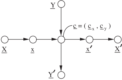
A CB net ${{\cal N}^{C}}$ is the HAS of QB net ${{\cal N}^{Q}}$ if ${{\cal N}^{Q}}$ and ${{\cal N}^{C}}$ have the same graph, and their node matrices are related as follows. For each node ${\underline{x}}_{i}$, if $A[x_{i}|(x.)_{\Gamma_{i}}]$ is the amplitude of node ${\underline{x}}_{i}$ in ${{\cal N}^{Q}}$, and $P[x_{i}|(x.)_{\Gamma_{i}}]$ is the probability of node ${\underline{x}}_{i}$ in ${{\cal N}^{C}}$, then $|A[x_{i}|(x.)_{\Gamma_{i}}]|^{2}=P[x_{i}|(x.)_{\Gamma_{i}}]$. In such a case, we will write ${\rm HAS}({{\cal N}^{Q}})={{\cal N}^{C}}$.

A unitary matrix $A(y,\tilde{x}|x,\tilde{y})$ (with rows labelled by $y,\tilde{x}$ and columns by $x,\tilde{y}$) is a q-embedding of probability matrix $P(y|x)$ if

$$\sum_{\tilde{x}}|A(y,\tilde{x}|x,\tilde{y}=0)|^{2}=P(y|x)\;$$ (113)

for all possible values of $y$ and $x$. (the “q” in “q-embedding” stands for “quantum”). We say $\tilde{y}$ is a source index and $\tilde{x}$ is a sink index. We also refer to $\tilde{x}$ and $\tilde{y}$ collectively as ancilla indices. Note that any unitary matrix is a q-embedding of its HAS. Indeed, in this case Eq.(113) is satisfied with the indices $\tilde{x}$ and $\tilde{y}$ each ranging over a single value (i.e., $\tilde{x}$ and $\tilde{y}$ are fixed). If a q-embedding satisfies $A(y,\tilde{x}|x,\tilde{y})\in Bool$ for all $y,\tilde{x},x,\tilde{y}$, we say that it is a deterministic q-embedding or a deterministic reversible extension (DRE) of its probability matrix (note that its probability matrix must also be deterministic). By an extension of a matrix we mean adding extra rows and/or columns to it. General q-embeddings use the square root of the entries of the original probability matrix so they are not simply extensions of the original matrix; they are, however, reversible since they are unitary matrices.

Given a QB net ${{\cal N}^{Q}}$, let

$$P[(x.)_{L}]=\left|\sum_{(x.)_{\Gamma_{Q}-L}}A(x.)\right|^{2}\;.$$ (114)

On the right hand side of Eq.(114), $A(x.)$ is the amplitude of story $(x.)$, $\Gamma_{Q}$ is the set of indices of all the nodes of ${{\cal N}^{Q}}$, and $L$ is the set of indices of all leaf (aka external) nodes of ${{\cal N}^{Q}}$. We say ${{\cal N}^{Q}}$ is a q-embedding of CB net ${{\cal N}^{C}}$ if $P[(x.)_{L}]$ defined by Eq.(114) satisfies

$$P[(x.)_{\Gamma_{C}}]=\sum_{L_{1}}P[(x.)_{L}]\;,$$ (115)

where $L_{1}\subset L$, and $\Gamma_{C}$ is the set of indices of all nodes of ${{\cal N}^{C}}$. Thus, the probability distribution associated with all nodes of ${{\cal N}^{C}}$ can be obtained from the probability distribution associated with the external nodes of ${{\cal N}^{Q}}$. Some examples of q-embeddings of CB nets have already been given during our discussion of standard algorithms. More examples will be given in subsequent sections.

For some positive integers $r$ and $s$, we will say a map $f:Bool^{r}\rightarrow Bool^{s}$ is a binary gate from $r$ to $s$ bits. $f$ uniquely specifies (and is uniquely specified) by the deterministic probability matrix with entries $P(y|x)=\delta(f(x),y)$, where $x=(x_{0},x_{1},\dots,x_{r-1})\in Bool^{r}$ and $y=(y_{0},y_{1},\dots,y_{s-1})\in Bool^{s}$. If $f$ is an invertible map, we will say that the gate is reversible. For example, the AND gate which takes $(x_{1},x_{0})\rightarrow y_{0}$ with $y_{0}=x_{0}x_{1}$ is a binary gate. So are the OR and NOT gates. Out of these 3 gates, only the NOT gate is reversible.

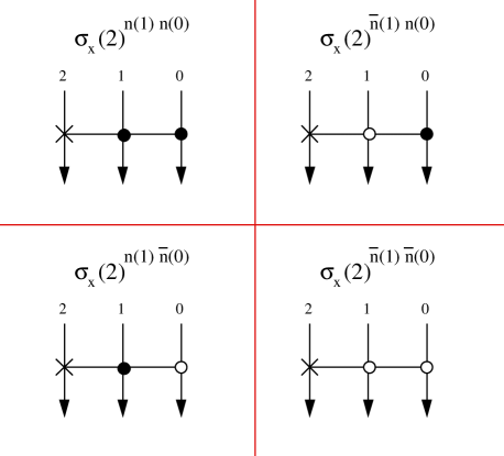
Another example of a reversible binary gate is the Toffoli gate[6]. It maps 3 bits into 3 bits as follows:

$$\begin{array}[]{l}y_{0}=T_{0}(x)=x_{0},\\ y_{1}=T_{1}(x)=x_{1},\\ y_{2}=T_{2}(x)=x_{2}\oplus x_{0}x_{1}.\end{array}\;$$ (116)

The Toffoli gate can also be defined as the following deterministic probability matrix

$$P(y|x)=\delta(y,T(x))=\delta(y_{2},x_{2}\oplus x_{0}x_{1})\delta(y_{1},x_{1})\delta(y_{0},x_{0})\;.$$ (117)

Consider 3 bits labelled 0, 1, and 2, and suppose the $i$th bit changes value from $x_{i}$ to $y_{i}$. Then bits 0 and 1 do not change whereas bit 2 flips iff the product $x_{0}x_{1}$ equals one. Thus, the probability matrix with entries given by Eq.(117) is simply a doubly controlled not:

$$[P(y|x)]=\sigma_{x}(2)^{{n}(1){n}(0)}\;.$$ (118)

It is convenient to use the term Toffoli gate to refer not only to the gate defined by Eq.(117), but also to the 3 other gates that one obtains by replacing $x_{0}x_{1}$ in Eq.(117) by $x_{0}\overline{x_{1}}$, or $\overline{x_{0}}x_{1}$, or $\overline{x_{0}}\overline{x_{1}}$. This corresponds to replacing ${n}(1){n}(0)$ in Eq.(118) by ${n}(1){\overline{n}}(0)$, or ${\overline{n}}(1){n}(0)$, or ${\overline{n}}(1){\overline{n}}(0)$. Fig.8 shows the 4 doubly-controlled nots that we call Toffoli gates as well as the circuit diagrams usually used to represent them.

Figure 8: Four different kinds of Toffoli gates. 0,1,2 are bit labels.

Figure 9: How to express elementary gates in terms of Toffoli gates. $x_{0},x_{1},x_{2}\in Bool$ are bit values.

5.1 Q-Embedding of Probability Matrices

In this section we will first give some examples of q-embeddings of probability matrices. Then we will show that any probability matrix has a q-embedding.

Any unitary matrix is a q-embedding of its HAS, but such q-embeddings are trivial in the sense that they have no ancilla indices.

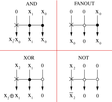
As first shown in Refs.[6], the Toffoli gates can be used to build q-embeddings (in fact, DREs) of the elementary binary gates AND, XOR, NOT, FANOUT. See Fig.9. Let $x=(x_{0},x_{1},x_{2})\in Bool^{3}$ and $y=(y_{0},y_{1},y_{2})\in Bool^{3}$. For the AND gate,

$$\sum_{y_{1},y_{0}}\left|\langle y|\sigma_{x}(2)^{{n}(1){n}(0)}|x_{2}=0,x_{1},x_{0}\rangle\right|^{2}=\delta(y_{2},x_{1}x_{0})\;.$$ (119a)

For the FANOUT gate,

$$\sum_{y_{1}}\left|\langle y|\sigma_{x}(2)^{{\overline{n}}(1){n}(0)}|x_{2}=0,x_{1}=0,x_{0}\rangle\right|^{2}=\delta(y_{2},x_{0})\delta(y_{0},x_{0})\;.$$ (119b)

For the XOR gate,

$$\sum_{y_{1},y_{0}}\left|\langle y|\sigma_{x}(2)^{{n}(1){\overline{n}}(0)}|x_{2},x_{1},x_{0}=0\rangle\right|^{2}=\delta(y_{2},x_{2}\oplus x_{1})\;.$$ (119c)

For the NOT gate,

$$\sum_{y_{1},y_{0}}\left|\langle y|\sigma_{x}(2)^{{\overline{n}}(1){\overline{n}}(0)}|x_{2},x_{1}=0,x_{0}=0\rangle\right|^{2}=\delta(y_{2},x_{2}\oplus 1)=\delta(y_{2},\overline{x_{2}})\;.$$ (119d)

Note that the NOT gate is just $\sigma_{x}$, which is a DRE of itself. Eq.(119d) gives a different DRE of $\sigma_{x}$. In the left hand side of Eqs.(119), the $x_{i}$ indices that are set to zero are called source indices, and the $y_{i}$ indices that are summed over are called sink indices. Sink and source indices are collectively called ancilla indices.

Next we will prove that any probability matrix has a q-embedding. Suppose that we are given a probability matrix $P(y|x)$ where $x\in S_{\underline{x}}$ and $y\in S_{\underline{y}}$. Let $N_{\underline{x}}$ (ditto, $N_{\underline{y}}$) denote the number of elements in $S_{\underline{x}}$ (ditto, $S_{\underline{y}}$). Let $\xi^{(x)}$ for $x\in S_{\underline{x}}$ be any orthonormal basis of the complex $N_{\underline{x}}$ dimensional vector space. The components of $\xi^{(x)}$ will be denoted by $\xi^{(x)}_{\tilde{x}}$, where $\tilde{x}\in S_{\underline{x}}$. If the $\xi^{(x)}$’s are the standard basis, then $\xi^{(x)}_{\tilde{x}}=\delta(x,\tilde{x})$. Define matrix $A$ by

$$A(y,\tilde{x}|x,\tilde{y})=\left\{\begin{array}[]{ll}\sqrt{P(y|x)}\;\;\xi^{x}_{\tilde{x}}&\mbox{ if}\;\tilde{y}=0\\ \mbox{obtained by Gram-Schmidt method}&\mbox{ if}\;\tilde{y}\neq 0\end{array}\right.\;.$$ (120)

Figure 10: How to construct a q-embedding of any probability matrix.

To understand the last equation, consider Fig.10. In that figure we have assumed for definiteness that $S_{\underline{x}}=\{0,1,2\}$ and $S_{\underline{y}}=\{0,1,2,3\}$. The shaded (ditto, unshaded) columns have $\tilde{y}\neq 0$ (ditto, $\tilde{y}=0$). It is easy to see that the unshaded columns are orthonormal because the vectors $\xi^{x}$ are orthonormal and $\sum_{y}P(y|x)=1$. Since the unshaded columns are orthonormal, one can use the Gram-Schmidt method[10] to fill the shaded columns so that all the columns of $A$ are orthonormal and therefore $A$ is unitary. Note that by virtue of Eq.(120),

$$\sum_{\tilde{x}}|A(y,\tilde{x}|x,\tilde{y}=0)|^{2}=\sum_{\tilde{x}}P(y|x)\xi^{(x)*}_{\tilde{x}}\xi^{(x)}_{\tilde{x}}=P(y|x)\;$$ (121)

so that the $A$ defined by Eq.(120) does indeed satisfy Eq.(113).[16]

Note that the matrix $A$ defined by Eq.(120) has dimensions $N_{\underline{x}}N_{\underline{y}}\times N_{\underline{x}}N_{\underline{y}}$. It is sometimes possible to find a smaller q-embedding of an $N_{\underline{y}}\times N_{\underline{x}}$ probability matrix $P(y|x)$. For example, $\sigma_{x}$ is a q-embedding of itself. As a less trivial example, suppose

$$P(y|x_{1},x_{2})=\delta(y,x_{1}\oplus x_{2})\;,$$ (122)

for $y,x_{1},x_{2}\in Bool$. Then define

$$A(y,e|x_{1},x_{2})=\frac{(-1)^{x_{1}e}}{\sqrt{2}}\delta(y,x_{1}\oplus x_{2})\;,$$ (123)

for $y,e,x_{1},x_{2}\in Bool$. It is easy to check that matrix $A$ is unitary. Furthermore,

$$\sum_{e}|A(y,e|x_{1},x_{2})|^{2}=\frac{1}{2}\sum_{e}\delta(y,x_{1}\oplus x_{2})=\delta(y,x_{1}\oplus x_{2})\;.$$ (124)

5.2 Q-Embedding of CB Nets

As we’ve said before, F-T showed in Refs.[6] how, given any binary gate $f$, one can construct another binary gate $\overline{f}$ such that $\overline{f}$ is a DRE of $f$. Their method for constructing $\overline{f}$ is to first represent $f$ as a binary deterministic circuit composed of elementary gates (AND, XOR, NOT, FANOUT), and then to modify the circuit by replacing each of its gates by a DRE of it. The desired gate $\overline{f}$ is then specified by the modified circuit.

In this section we will show how, given any CB net ${{\cal N}^{C}}$, one can construct a QB net ${{\cal N}^{Q}}$ which is a q-embedding of ${{\cal N}^{C}}$. So far we’ve shown how to construct a q-embedding for any probability matrix. Now remember that each node of ${{\cal N}^{C}}$ has a probability matrix assigned to it. The main step in constructing a q-embedding of ${{\cal N}^{C}}$ is to replace each node matrix of ${{\cal N}^{C}}$ with a q-embedding of it. Thus, our method for constructing a q-embedding of a CB net is a generalization of the F-T method for constructing a DRE of a binary deterministic circuit. We generalize their method so that it can be applied to any classical stochastic circuit, not just binary deterministic ones.

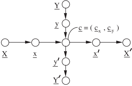
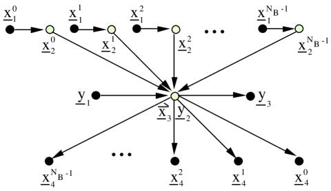
Before describing our construction method, we need some definitions. We say a node ${\underline{m}}$ is a marginalizer node if it has a single input arrow and a single output arrow. Furthermore, the parent node of ${\underline{m}}$, call it ${\underline{x}}$, has states $x=(x_{1},x_{2},\ldots,x_{n})$, where $x_{i}\in S_{{\underline{x}}_{i}}$ for each $i\in Z_{1,n}$. Furthermore, for some particular integer $i_{0}\in Z_{1,n}$, the set of possible states of ${\underline{m}}$ is $S_{\underline{m}}=S_{{\underline{x}}_{i_{0}}}$, and the node matrix of ${\underline{m}}$ is $P({\underline{m}}=m|{\underline{x}}=x)=\delta(m,x_{i_{0}})$.

Let ${{\cal N}^{C}}$ be a CB net for which we want to obtain a q-embedding. Our construction has two steps:

(Step 1) Add marginalizer nodes.

More specifically, replace ${{\cal N}^{C}}$ by a modified CB net ${{\cal N}^{C}}_{mod}$ obtained as follows. For each node ${\underline{x}}$ of ${{\cal N}^{C}}$, add a marginalizer node between ${\underline{x}}$ and every child of ${\underline{x}}$. If ${\underline{x}}$ has no children, add a child to it.

As an example of this step, consider the net ${{\cal N}^{C}}$ (“two body scattering net”) defined by Fig.11 and Table 5.2.

Figure 11: CB net for 2-body scattering. We show how to construct a q-embedding for this CB net.

nodes	states	probabilities	comments
${\underline{a}}$	$a\in S_{\underline{a}}$	$P(a)$
${\underline{b}}$	$b\in S_{\underline{b}}$	$P(b)$
${\underline{c}}$	$c\in S_{\underline{c}}$	$P(c|x)$
${\underline{d}}$	$d\in S_{\underline{d}}$	$P(d|x)$
${\underline{x}}$	$x\in S_{\underline{x}}$	$P(x|a,b)$

Table 7

Applying Step 1 to ${{\cal N}^{C}}$ for two body scattering yields ${{\cal N}^{C}}_{mod}$ defined by Fig.12 and Table 5.2.

Figure 12: CB net of Fig.11 after adding marginalizer nodes.

nodes	states	probabilities	comments
${\underline{a}}_{2}$	$a_{2}\in S_{\underline{a}}$	$P_{\underline{a}}(a_{2})$
${\underline{a}}_{3}$	$a_{3}\in S_{\underline{a}}$	$\delta(a_{3},a_{2})$
${\underline{b}}_{2}$	$b_{2}\in S_{\underline{b}}$	$P_{\underline{b}}(b_{2})$
${\underline{b}}_{3}$	$b_{3}\in S_{\underline{b}}$	$\delta(b_{3},b_{2})$
${\underline{c}}_{2}$	$c_{2}\in S_{\underline{c}}$	$P_{{\underline{c}}|{\underline{x}}}(c_{2}|x_{3c})$
${\underline{c}}_{3}$	$c_{3}\in S_{\underline{c}}$	$\delta(c_{3},c_{2})$
${\underline{d}}_{2}$	$d_{2}\in S_{\underline{d}}$	$P_{{\underline{d}}|{\underline{x}}}(d_{2}|x_{3d})$
${\underline{d}}_{3}$	$d_{3}\in S_{\underline{d}}$	$\delta(d_{3},d_{2})$
$({\underline{x}}_{2c},{\underline{x}}_{2d})$	$(x_{2c},x_{2d})\in S_{\underline{x}}^{2}$	$P_{{\underline{x}}|{\underline{a}},{\underline{b}}}(x_{2c}|a_{3},b_{3})\delta(x_{2d},x_{2c})$
${\underline{x}}_{3c}$	$x_{3c}\in S_{\underline{x}}$	$\delta(x_{3c},x_{2c})$
${\underline{x}}_{3d}$	$x_{3d}\in S_{\underline{x}}$	$\delta(x_{3d},x_{2d})$

Table 8

(Step 2) Replace node probability matrices by their q-embeddings. Add ancilla nodes.

More specifically, replace ${{\cal N}^{C}}_{mod}$ by a QB net ${{\cal N}^{Q}}$ obtained as follows. For each node of ${{\cal N}^{C}}_{mod}$, except for the marginalizer nodes that were added in the previous step, replace its node matrix by a new node matrix which is a q-embedding of the original node matrix. Add a new node for each ancilla index of each new node matrix. These new nodes will be called ancilla nodes (of either the source or sink type) because they correspond to ancilla indices.

Applying Step 2 to net ${{\cal N}^{C}}_{mod}$ for two body scattering yields ${{\cal N}^{Q}}$ defined by Fig.13 and Table 5.2.

Figure 13: A QB Net which is a q-embedding for the CB net of Fig.11.

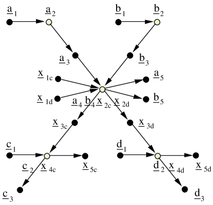
nodes	states	amplitudes	comments
${\underline{a}}_{1}$	$a_{1}\in S_{\underline{a}}$	$\delta(a_{1},0)$
${\underline{a}}_{2}$	$a_{2}\in S_{\underline{a}}$	$A(a_{2}|a_{1}=0)=\sqrt{P_{\underline{a}}(a_{2})}$
${\underline{a}}_{3}$	$a_{3}\in S_{\underline{a}}$	$\delta(a_{3},a_{2})$
$({\underline{a}}_{4},{\underline{b}}_{4},{\underline{x}}_{2c},{\underline{x}}_{2d})$	$(a_{4},b_{4},x_{2c},x_{2d})\in S_{{\underline{a}},{\underline{b}},{\underline{x}},{\underline{x}}}$	$A(a_{4},b_{4},x_{2c},x_{2d}|a_{3},b_{3},x_{1c}=0,x_{1d}=0)=$
		$\sqrt{P_{{\underline{x}}|{\underline{a}},{\underline{b}}}(x_{2c}|a_{3},b_{3})}\delta(a_{4},a_{3})\delta(b_{4},b_{3})\delta(x_{2d},x_{2c})$
${\underline{a}}_{5}$	$a_{5}\in S_{{\underline{a}}}$	$\delta(a_{5},a_{4})$
${\underline{b}}_{1}$	$b_{1}\in S_{\underline{b}}$	$\delta(b_{1},0)$
${\underline{b}}_{2}$	$b_{2}\in S_{\underline{b}}$	$A(b_{2}|b_{1}=0)=\sqrt{P_{\underline{b}}(b_{2})}$
${\underline{b}}_{3}$	$b_{3}\in S_{\underline{b}}$	$\delta(b_{3},b_{2})$
${\underline{b}}_{5}$	$b_{5}\in S_{{\underline{b}}}$	$\delta(b_{5},b_{4})$
${\underline{c}}_{1}$	$c_{1}\in S_{\underline{c}}$	$\delta(c_{1},0)$
$({\underline{c}}_{2},{\underline{x}}_{4c})$	$(c_{2},x_{4c})\in S_{{\underline{c}},{\underline{x}}}$	$A(c_{2},x_{4c}|c_{1}=0,x_{3c})=$
		$\sqrt{P_{{\underline{c}}|{\underline{x}}}(c_{2}|x_{3c})}\delta(x_{4c},x_{3c})$
${\underline{c}}_{3}$	$c_{3}\in S_{\underline{c}}$	$\delta(c_{3},c_{2})$
${\underline{d}}_{1}$	$d_{1}\in S_{\underline{d}}$	$\delta(d_{1},0)$
$({\underline{d}}_{2},{\underline{x}}_{4d})$	$(d_{2},x_{4d})\in S_{{\underline{d}},{\underline{x}}}$	$A(d_{2},x_{4d}|d_{1}=0,x_{3d})=$
		$\sqrt{P_{{\underline{d}}|{\underline{x}}}(d_{2}|x_{3d})}\delta(x_{4d},x_{3d})$
${\underline{d}}_{3}$	$d_{3}\in S_{\underline{d}}$	$\delta(d_{3},d_{2})$
${\underline{x}}_{1c}$	$x_{1c}\in S_{{\underline{x}}}$	$\delta(x_{1c},0)$
${\underline{x}}_{1d}$	$x_{1d}\in S_{{\underline{x}}}$	$\delta(x_{1d},0)$
${\underline{x}}_{3c}$	$x_{3c}\in S_{\underline{x}}$	$\delta(x_{3c},x_{2c})$
${\underline{x}}_{3d}$	$x_{3d}\in S_{\underline{x}}$	$\delta(x_{3d},x_{2d})$
${\underline{x}}_{5c}$	$x_{5c}\in S_{\underline{x}}$	$\delta(x_{5c},x_{4c})$
${\underline{x}}_{5d}$	$x_{5d}\in S_{\underline{x}}$	$\delta(x_{5d},x_{4d})$

Table 9

${{\cal N}^{Q}}$ looks much more complicated than ${{\cal N}^{C}}$, but it really isn’t, since most of its node matrices are delta functions which quickly disappear when adding over node states.

According to Table 5.2, the probability amplitude for the external (aka leaf) nodes is given by

$$\begin{array}[]{l}A(a_{5},b_{5},c_{3},d_{3},x_{5c},x_{5d})=\\ =\sum_{\cdot}\sqrt{P_{{\underline{a}}}(\mbox{\@text@daccent{{\it a}}}_{2})P_{{\underline{b}}}(\mbox{\@text@daccent{{\it b}}}_{2})P_{{\underline{x}}|{\underline{a}},{\underline{b}}}(\mbox{\@text@daccent{{\it x}}}_{2c}|\mbox{\@text@daccent{{\it a}}}_{3},\mbox{\@text@daccent{{\it b}}}_{3})P_{{\underline{c}}|{\underline{x}}}(\mbox{\@text@daccent{{\it c}}}_{2}|\mbox{\@text@daccent{{\it x}}}_{3c})P_{{\underline{d}}|{\underline{x}}}(\mbox{\@text@daccent{{\it d}}}_{2}|\mbox{\@text@daccent{{\it x}}}_{3d})}\\ \;\;\;\;\theta(\mbox{\@text@daccent{{\it a}}}_{2}=\mbox{\@text@daccent{{\it a}}}_{3}=\mbox{\@text@daccent{{\it a}}}_{4}=a_{5})\theta(\mbox{\@text@daccent{{\it b}}}_{2}=\mbox{\@text@daccent{{\it b}}}_{3}=\mbox{\@text@daccent{{\it b}}}_{4}=b_{5})\\ \;\;\;\;\theta(\mbox{\@text@daccent{{\it x}}}_{2c}=\mbox{\@text@daccent{{\it x}}}_{3c}=\mbox{\@text@daccent{{\it x}}}_{4c}=x_{5c})\theta(\mbox{\@text@daccent{{\it x}}}_{2d}=\mbox{\@text@daccent{{\it x}}}_{3d}=\mbox{\@text@daccent{{\it x}}}_{4d}=x_{5d})\theta(x_{5c}=x_{5d})\\ \;\;\;\;\theta(\mbox{\@text@daccent{{\it c}}}_{2}=c_{3})\theta(\mbox{\@text@daccent{{\it d}}}_{2}=d_{3})\\ \;\;\;\;\theta(\mbox{\@text@daccent{{\it a}}}_{1}=\mbox{\@text@daccent{{\it b}}}_{1}=\mbox{\@text@daccent{{\it c}}}_{1}=\mbox{\@text@daccent{{\it d}}}_{1}=\mbox{\@text@daccent{{\it x}}}_{1c}=\mbox{\@text@daccent{{\it x}}}_{1d}=0)\end{array}\;,$$ (125)

where we have summed over all internal (non-leaf) nodes. Eq.(125) immediately reduces to

$$\begin{array}[]{l}A(a_{5},b_{5},c_{3},d_{3},x_{5c},x_{5d})=\\ =\sqrt{P_{{\underline{a}}}(a_{5})P_{{\underline{b}}}(b_{5})P_{{\underline{x}}|{\underline{a}},{\underline{b}}}(x_{5c}|a_{5},b_{5})P_{{\underline{c}}|{\underline{x}}}(c_{3}|x_{5c})P_{{\underline{d}}|{\underline{x}}}(d_{3}|x_{5d})}\theta(x_{5c}=x_{5d})\end{array}\;.$$ (126)

Eq.(126) shows that the net ${{\cal N}^{Q}}$ that we constructed from the net ${{\cal N}^{C}}$ by following steps 1 and 2 satisfies the definition Eq.(115) that we gave earlier for a q-embedding of ${{\cal N}^{C}}$. The probability distribution of the states of the external nodes of the QB net ${{\cal N}^{Q}}$ contains all the probabilistic information of the original CB net ${{\cal N}^{C}}$. Hurray!

From Eq.(126), it is clear that by running ${{\cal N}^{Q}}$ on a quantum computer (or similar quantum system), we can calculate any conditional probability that one would want to calculate for ${{\cal N}^{C}}$. For example, suppose we wanted to calculate $P_{{\underline{a}},{\underline{d}}|{\underline{x}}}$. Run ${{\cal N}^{Q}}$ on the quantum computer several times, each time measuring nodes ${\underline{a}}_{5},{\underline{d}}_{3}$ and ${\underline{x}}_{5d}$ and not measuring all other external nodes. The resulting measurements will be distributed according to $P_{{\underline{a}},{\underline{d}},{\underline{x}}}$. Taking the magnitude squared of the amplitude and summing the result over the states of the un-measured external nodes will be performed automatically by Nature. The laws of quantum mechanics guarantee it. Proceed in the same way to calculate $P_{{\underline{x}}}$. Run ${{\cal N}^{Q}}$ on the quantum computer several times, each time measuring node ${\underline{x}}_{5d}$ and not measuring all other external nodes. Finally divide $P_{{\underline{a}},{\underline{d}},{\underline{x}}}$ by $P_{{\underline{x}}}$ on a classical (or quantum?) computer.

The q-embedding of a CB net, as defined by Eq.(115), is not unique. For example, we could have defined the net ${{\cal N}^{Q}}$ given by Fig.13 without nodes ${\underline{a}}_{3}$ and ${\underline{b}}_{3}$. We chose to include such nodes for pedagogical reasons.

To run a QB net on a quantum computer, we need to replace the QB net by an equivalent SEO that a quantum computer can understand. This can be done with the help of a quantum compiler [9][8]. One could compile individually each node representing a q-embedding, or one could compile whole subgraphs of the QB net all at once. Note that it may suffice to find a SEO that is only approximately (within a certain precision) equivalent instead of exactly equivalent to the QB net. This may be true if, for example, the probabilities associated with the CB net that was q-embedded were not specified too precisely to begin with.

Suppose $a_{1},a_{2},\ldots a_{\nu}$ belong to a finite set $S_{\underline{a}}$, and suppose that they are distributed according to a probability distribution $P_{\underline{a}}$. What number $\nu$ of samples $a_{i}$ is necessary to estimate $P_{\underline{a}}$ within a given precision? This question is directly relevant to our method for estimating probabilities by running a QB net on a quantum computer. We will not give a detailed answer to this question here. For an answer, the reader can consult any book on the mathematical theory of Statistics. An imprecise rule of thumb is that if the support of $P_{\underline{a}}$ has $\nu_{0}$ elements, then $\nu$ must be at least as large as $\nu_{0}$; i.e., one needs at least “one data point per bin” to estimate $P_{\underline{a}}$ with any decent accuracy.

We have given a method for calculating, via a quantum computer, the conditional probabilities associated with a CB net. Does our method have an advantage in time complexity with respect to classical methods for calculating the same probabilities? We will not give a detailed answer to this question here. The answer must be yes, sometimes. After all, our method generalizes the algorithms by Deutsch-Jozsa, Simon, Grover, etc., and these are known to have a complexity advantage.

To conclude this section, we will present a second, more complicated example of our method of finding a q-embedding for a CB net. A CB net (first given in Ref.[17]) for lung disease diagnosis is defined by Fig.14 and Table 5.2.

Figure 14: CB net for lung disease diagnosis. We show how to construct a q-embedding for this CB net.

nodes	states	probabilities	comments
${\underline{a}}$	$a\in Bool$	$P({\underline{a}}=1)=.01$	Visited Asia?
${\underline{b}}$	$b\in Bool$	$\begin{array}[]{l}P({\underline{b}}=1|{\underline{s}}=1)=.60\\ P({\underline{b}}=1|{\underline{s}}=0)=.30\end{array}$	Bronchitis?
${\underline{d}}$	$d\in Bool$	$\begin{array}[]{l}P({\underline{d}}=1|{\underline{e}}=1,{\underline{b}}=1)=.90\\ P({\underline{d}}=1|{\underline{e}}=1,{\underline{b}}=0)=.70\\ P({\underline{d}}=1|{\underline{e}}=0,{\underline{b}}=1)=.80\\ P({\underline{d}}=1|{\underline{e}}=0,{\underline{b}}=0)=.10\end{array}$	Dyspnea(trouble breathing)?
${\underline{e}}$	$e\in Bool$	$P(e|l,t)=\delta(e,l\vee t)$	Either TB or Lung Cancer?
${\underline{l}}$	$l\in Bool$	$\begin{array}[]{l}P({\underline{l}}=1|{\underline{s}}=1)=.10\\ P({\underline{l}}=1|{\underline{s}}=0)=.01\end{array}$	Lung Cancer?
${\underline{s}}$	$s\in Bool$	$P({\underline{s}}=1)=.5$	Smokes?
${\underline{t}}$	$t\in Bool$	$\begin{array}[]{l}P({\underline{t}}=1|{\underline{a}}=1)=.05\\ P({\underline{t}}=1|{\underline{a}}=0)=.01\end{array}$	Tuberculosis?
${\underline{x}}$	$x\in Bool$	$\begin{array}[]{l}P({\underline{x}}=1|{\underline{e}}=1)=.98\\ P({\underline{x}}=1|{\underline{e}}=0)=.05\end{array}$	Positive X-ray?

Table 10

If one follows the two steps that were described earlier in this section, one obtains the QB net defined by Fig.15 and Table 5.2.

Figure 15: A QB Net which is a q-embedding for the CB net of Fig.14.

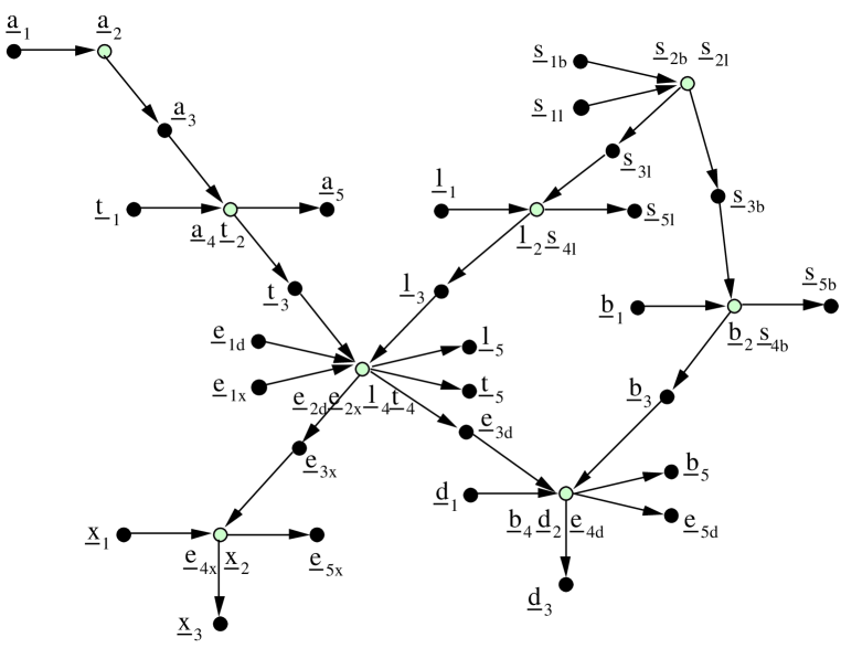
nodes	states	amplitudes
${\underline{a}}_{1}$	$a_{1}\in Bool$	$\delta(a_{1},0)$
${\underline{a}}_{2}$	$a_{2}\in Bool$	$A(a_{2}|a_{1}=0)=\sqrt{P_{\underline{a}}(a_{2})}$
${\underline{a}}_{3}$	$a_{3}\in Bool$	$\delta(a_{3},a_{2})$
$({\underline{a}}_{4},{\underline{t}}_{2})$	$(a_{4},t_{2})\in Bool^{2}$	$A(a_{4},t_{2}|a_{3},t_{1}=0)=\sqrt{P_{{\underline{t}}|{\underline{a}}}(t_{2}|a_{3})}\delta(a_{4},a_{3})$
${\underline{a}}_{5}$	$a_{5}\in Bool$	$\delta(a_{5},a_{4})$
${\underline{b}}_{1}$	$b_{1}\in Bool$	$\delta(b_{1},0)$
$({\underline{b}}_{2},{\underline{s}}_{4b})$	$(b_{2},s_{4b})\in Bool^{2}$	$A(b_{2},s_{4b}|b_{1}=0,s_{3b})=\sqrt{P_{{\underline{b}}|{\underline{s}}}(b_{2}|s_{3b})}\delta(s_{4b},s_{3b})$
${\underline{b}}_{3}$	$b_{3}\in Bool$	$\delta(b_{3},b_{2})$
$({\underline{b}}_{4},{\underline{d}}_{2},{\underline{e}}_{4d})$	$(b_{4},d_{2},e_{4d})\in Bool^{3}$	$A(b_{4},d_{2},e_{4d}|b_{3},d_{1}=0,e_{3d})=\sqrt{P_{{\underline{d}}|{\underline{b}},{\underline{e}}}(d_{2}|b_{3},e_{3d})}\delta(b_{4},b_{3})\delta(e_{4d},e_{3d})$
${\underline{b}}_{5}$	$b_{5}\in Bool$	$\delta(b_{5},b_{4})$
${\underline{d}}_{1}$	$d_{1}\in Bool$	$\delta(d_{1},0)$
${\underline{d}}_{3}$	$d_{3}\in Bool$	$\delta(d_{3},d_{2})$
${\underline{e}}_{1d}$	$e_{1d}\in Bool$	$\delta(e_{1d},0)$
${\underline{e}}_{1x}$	$e_{1x}\in Bool$	$\delta(e_{1x},0)$
$({\underline{e}}_{2d},{\underline{e}}_{2x},{\underline{l}}_{4},{\underline{t}}_{4})$	$(e_{2d},e_{2x},l_{4},t_{4})$	$A(e_{2d},e_{2x},l_{4},t_{4}|e_{1d}=0,e_{1x}=0,l_{3},t_{3})=$
	$\in Bool^{4}$	$\sqrt{P_{{\underline{e}}|{\underline{l}},{\underline{t}}}(e_{2d}|l_{3},t_{3})}\delta(e_{2x},e_{2d})\delta(l_{4},l_{3})\delta(t_{4},t_{3})$
${\underline{e}}_{3d}$	$e_{3d}\in Bool$	$\delta(e_{3d},e_{2d})$
${\underline{e}}_{3x}$	$e_{3x}\in Bool$	$\delta(e_{3x},e_{2x})$
$({\underline{e}}_{4x},{\underline{x}}_{2})$	$(e_{4x},x_{2})\in Bool^{2}$	$A(e_{4x},x_{2}|e_{3x},x_{1}=0)=\sqrt{P_{{\underline{x}}|{\underline{e}}}(x_{2}|e_{3x})}\delta(e_{4x},e_{3x})$
${\underline{e}}_{5d}$	$e_{5d}\in Bool$	$\delta(e_{5d},e_{4d})$
${\underline{e}}_{5x}$	$e_{5x}\in Bool$	$\delta(e_{5x},e_{4x})$
${\underline{l}}_{1}$	$l_{1}\in Bool$	$\delta(l_{1},0)$
$({\underline{l}}_{2},{\underline{s}}_{4l})$	$(l_{2},s_{4l})\in Bool^{2}$	$A(l_{2},s_{4l}|l_{1}=0,s_{3l})=\sqrt{P_{{\underline{l}}|{\underline{s}}}(l_{2}|s_{3l})}\delta(s_{4l},s_{3l})$
${\underline{l}}_{3}$	$l_{3}\in Bool$	$\delta(l_{3},l_{2})$
${\underline{l}}_{5}$	$l_{5}\in Bool$	$\delta(l_{5},l_{4})$
${\underline{s}}_{1b}$	$s_{1b}\in Bool$	$\delta(s_{1b},0)$
${\underline{s}}_{1l}$	$s_{1l}\in Bool$	$\delta(s_{1l},0)$
$({\underline{s}}_{2b},{\underline{s}}_{2l})$	$(s_{2b},s_{2l})\in Bool^{2}$	$A(s_{2b},s_{2l}|s_{1b}=0,s_{1l}=0)=\sqrt{P_{{\underline{s}}}(s_{2b})}\delta(s_{2l},s_{2b})$
${\underline{s}}_{3b}$	$s_{3b}\in Bool$	$\delta(s_{3b},e_{2b})$
${\underline{s}}_{3l}$	$s_{3l}\in Bool$	$\delta(s_{3l},s_{2l})$
${\underline{s}}_{5b}$	$s_{5b}\in Bool$	$\delta(s_{5b},s_{4b})$
${\underline{s}}_{5l}$	$s_{5l}\in Bool$	$\delta(s_{5l},s_{4l})$
${\underline{t}}_{1}$	$t_{1}\in Bool$	$\delta(t_{1},0)$
${\underline{t}}_{3}$	$t_{3}\in Bool$	$\delta(t_{3},t_{2})$
${\underline{t}}_{5}$	$t_{5}\in Bool$	$\delta(t_{5},t_{4})$
${\underline{x}}_{1}$	$x_{1}\in Bool$	$\delta(x_{1},0)$
${\underline{x}}_{3}$	$x_{3}\in Bool$	$\delta(x_{3},x_{2})$

Table 11

According to Table 5.2, the probability amplitude for the external (aka leaf) nodes is given by

$$\begin{array}[]{l}A(a_{5},b_{5},d_{3},e_{5d},e_{5x},l_{5},s_{5b},s_{5l},t_{5},x_{3})=\\ =\sqrt{P_{{\underline{a}}}(a_{5})P_{{\underline{t}}|{\underline{a}}}(t_{5}|a_{5})P_{{\underline{b}}|{\underline{s}}}(b_{5}|s_{5b})P_{{\underline{d}}|{\underline{b}},{\underline{e}}}(d_{3}|b_{5},e_{5d})P_{{\underline{e}}|{\underline{l}},{\underline{t}}}(e_{5d}|l_{5},t_{5})P_{{\underline{x}}|{\underline{e}}}(x_{3}|e_{5d})P_{{\underline{l}}|{\underline{s}}}(l_{5}|s_{5l})P_{\underline{s}}(s_{5b})}\\ \;\;\;\;\theta(e_{5d},e_{5x})\theta(s_{5b},s_{5l})\end{array}\;.$$ (127)

6 Voting Net and Grover’s Microscope

In this section we will first present a CB net, call it ${{\cal N}^{C}}$, that describes voting. Then we will find a QB net ${{\cal N}^{Q}}$ that is a q-embedding of ${{\cal N}^{C}}$. In certain cases, the probabilities that we wish to find are too small to be measurable by running ${{\cal N}^{Q}}$ on a quantum computer. However, we will show that sometimes it is possible to define a new QB net, call it ${{\cal N}^{Q}}^{\prime}$, that magnifies and makes measurable the probabilities that were unmeasurable using ${{\cal N}^{Q}}$ alone. We will refer to ${{\cal N}^{Q}}^{\prime}$ as Grover’s Microscope for ${{\cal N}^{Q}}$, because ${{\cal N}^{Q}}^{\prime}$ is closely related to Grover’s algorithm, and it magnifies the probabilities found with ${{\cal N}^{Q}}$.

Suppose $y\in Bool$ and $\vec{x}=(x^{0},x^{1},\ldots,x^{{N_{B}}-1})\in Bool^{N_{B}}$. Consider the CB net (“voting net”) defined by Fig.16 and Table 6.

Figure 16: “Voting” CB net.

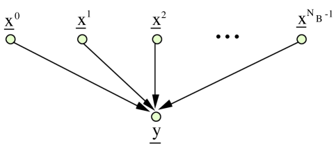
nodes	states	probabilities	comments
${\underline{x}}^{i}\;\;\mbox{for all}\;\;i\in Z_{0,{N_{B}}-1}$	$x^{i}\in Bool$	$P(x^{i})$
${\underline{y}}$	$y\in Bool$	$P(y|\vec{x})$

Table 12

Henceforth, we will abbreviate $P(y=0|\vec{x})=p_{i}$ and $P(y=1|\vec{x})=q_{i}$, where $i=dec(\vec{x})\in Z_{0,{N_{S}}-1}$. Hence $p_{i}+q_{i}=1$ for all $i\in Z_{0,{N_{S}}-1}$. In general, the probability matrix $P(y|\vec{x})$ has $2^{N_{B}}$ free parameters (namely, $p_{i}$ for all $i\in Z_{0,{N_{S}}-1}$). This number of parameters is a forbiddingly large for large ${N_{B}}$. To ease the task of specifying $P(y|\vec{x})$ , it is common to impose additional constraints on $P(y|\vec{x})$. An interesting special type of $P(y|\vec{x})$ is deterministic $pd(Bool|Bool^{N_{B}})$ matrices; that is, those that can be expressed in the form

$$P(y|\vec{x})=\delta(y,f(\vec{x}))\;,$$ (128)

where $f:Bool^{N_{B}}\rightarrow Bool$. In this case, the voting net can be used to pose the satisfiability problem (SAT): given $y=0$, find the most likely $\vec{x}\in Bool^{N_{B}}$; in other words, find those $\vec{x}$ for which $f(\vec{x})=0$. We say $f$ is AND-like if all $p_{i}$ equal zero except for one $p_{i}$ which equals one. For example, for ${N_{B}}=2$, if $f$ is an AND gate, then

$$P(y|\vec{x})_{AND}=\left\{\begin{array}[]{r}(x^{0},x^{1})\rightarrow\\ \begin{array}[]{llllll}&&\vline 00&01&10&11\\ \hline\cr y\downarrow&0&\vline 1&1&1&0\\ &1&\vline 0&0&0&1\\ \end{array}\end{array}\right.\;.$$ (129)

A slightly more general type of $P(y|\vec{x})$ is quasi-deterministic $pd(Bool|Bool^{N_{B}})$ matrices; that is, those that can be expressed in the form

$$P(y|\vec{x})=\sum_{\vec{t}}\delta(y,f(\vec{t}))P(t^{0}|x^{0})P(t^{1}|x^{1})\ldots P(t^{{N_{B}}-1}|x^{{N_{B}}-1})\;,$$ (130)

where $f:Bool^{N_{B}}\rightarrow Bool$ and we sum over all $\vec{t}=(t^{0},t^{1},\ldots,t^{{N_{B}}-1})\in Bool^{N_{B}}$. When $f(\vec{t})=t^{0}\vee t^{1}\vee\ldots\vee t^{{N_{B}}-1}$, $P(y|\vec{x})$ is called a noisy-OR. Appendix A discusses how to q-embed deterministic $pd(Bool|Bool^{N_{B}})$ matrices, and how to express such q-embeddings as a SEO . Appendix B discusses the same thing for quasi-deterministic $pd(Bool|Bool^{N_{B}})$ matrices.

A q-embedding for the CB net defined by Fig.16 and Table 6 is given by the QB net defined by Fig.17 and Table 6.

Figure 17: A QB Net which is a q-embedding for the CB net of Fig.16.

nodes	states	amplitudes	comments
$\vec{{\underline{x}}}_{1}$	$\vec{x}_{1}\in Bool^{N_{B}}$	$\delta(\vec{x}_{1},0)$
$\vec{{\underline{x}}}_{2}$	$\vec{x}_{2}\in Bool^{N_{B}}$	$A(\vec{x}_{2}|\vec{x}_{1}=0)=\sqrt{P_{\vec{{\underline{x}}}}(\vec{x}_{2})}$
$(\vec{{\underline{x}}}_{3},{\underline{y}}_{2})$	$(\vec{x}_{3},y_{2})\in Bool^{{N_{B}}+1}$	$A(\vec{x}_{3},y_{2}|\vec{x}_{2},y_{1}=0)=\sqrt{P_{{\underline{y}}|\vec{{\underline{x}}}}(y_{2}|\vec{x}_{2})}\delta(\vec{x}_{3},\vec{x}_{2})$
$\vec{{\underline{x}}}_{4}$	$\vec{x}_{4}\in Bool^{N_{B}}$	$\delta(\vec{x}_{4},\vec{x}_{3})$
${\underline{y}}_{1}$	$y_{1}\in Bool$	$\delta(y_{1},0)$
${\underline{y}}_{3}$	$y_{3}\in Bool$	$\delta(y_{3},y_{2})$

Table 13

According to Table 6, the probability amplitude for the leaf (external) nodes is

$$A(\vec{x}_{4},y_{3})=$$ (131a)

$$= \sum_{\cdot}\sqrt{P_{\vec{{\underline{x}}}}(\vec{\mbox{\@text@daccent{{\it x}}}}_{2})P_{{\underline{y}}|\vec{{\underline{x}}}}(\mbox{\@text@daccent{{\it y}}}_{2}|\vec{\mbox{\@text@daccent{{\it x}}}}_{2})}\theta(\mbox{\@text@daccent{{\it y}}}_{2}=y_{3})\theta(\vec{\mbox{\@text@daccent{{\it x}}}}_{2}=\vec{\mbox{\@text@daccent{{\it x}}}}_{3}=\vec{x}_{4})\theta(\vec{\mbox{\@text@daccent{{\it x}}}}_{1}=\mbox{\@text@daccent{{\it y}}}_{1}=0)$$

$$= \sqrt{P_{\vec{{\underline{x}}}}(\vec{x}_{4})P_{{\underline{y}}|\vec{{\underline{x}}}}(y_{3}|\vec{x}_{4})}\;.$$ (131b)

To fully specify the QB net for voting, we need to extend $A(\vec{x}_{2}|\vec{x}_{1}=0)$ and $A(\vec{x}_{3},y_{2}|\vec{x}_{2},y_{1}=0)$ into unitary matrices by adding columns to them. This can always be accomplished by applying the Gram-Schmidt algorithm. But sometimes one can guess a matrix extension and applying Gram-Schmidt becomes unnecessary. If $P_{\vec{{\underline{x}}}}$ is uniform (i.e., $P(\vec{x})=1/{N_{S}}$ for all $\vec{x}$, which means there is no a priori information about $\vec{x}$), then $A(\vec{x}_{2}|\vec{x}_{1}=0)=1/\sqrt{{N_{S}}}$. In this case, we can extend $A(\vec{x}_{2}|\vec{x}_{1}=0)$ into the unitary matrix

$$[A(\vec{x}_{2}|\vec{x}_{1})]=\hat{H}_{N_{B}}\;.$$ (132)

(This works because all entries of the first column of $\hat{H}_{N_{B}}$ are equal to $1/\sqrt{{N_{S}}}$.) As to extending $A(\vec{x}_{3},y_{2}|\vec{x}_{2},y_{1}=0)$, this can be done as follows. Define

$$\Delta_{p}=diag(\sqrt{p_{0}},\sqrt{p_{1}},\ldots,\sqrt{p_{{N_{S}}-1}})\;,$$ (133)

and

$$\Delta_{q}=diag(\sqrt{q_{0}},\sqrt{q_{1}},\ldots,\sqrt{q_{{N_{S}}-1}})\;.$$ (134)

A possible way of extending $A(\vec{x}_{3},y_{2}|\vec{x}_{2},y_{1}=0)$ into a unitary matrix is

$$[A(\vec{x}_{3},y_{2}|\vec{x}_{2},y_{1})]=\left(\begin{array}[]{cc}\Delta_{p}&-\Delta_{q}\\ \Delta_{q}&\Delta_{p}\end{array}\right)\;.$$ (135)

Unitary matrices of this kind are called D-matrices in Ref.[8]. Ref.[8] shows how to decompose any D-matrix into a SEO.

Earlier, we explained how to estimate a conditional probability for a CB net by running a QB net $\nu$ times on a quantum computer. If we wanted to find $P(y|x^{0},x^{1})$ for the voting CB net, then the number of runs $\nu$ required to estimate $P(y|x^{0},x^{1})$ with moderate accuracy would not be too onerous, because the domain of $P(y|x^{0},x^{1})$ is $Bool^{3}$, which contains only 8 points. But what if we wanted to estimate $P(y|\vec{x})$? For large ${N_{B}}$, the domain of $P(y|\vec{x})$ is very large ($2^{{N_{B}}+1}$ points). If the support of $P(y|\vec{x})$ occupies a large fraction of this domain, then the number of runs $\nu$ required to estimate $P(y|\vec{x})$ with moderate accuracy is forbiddingly large. However, there are some cases in which “Grover’s Microscope” can come to the rescue, by allowing us to amplify certain salient features of $P(y|\vec{x})$ so that they become measurable in only a few runs.

Next we will discuss Grover’s Microscope for the voting QB net defined by Fig.17 and Table 6. For simplicity, we will assume that $P_{\vec{{\underline{x}}}}$ is uniform.

Let $\vec{\kappa}=(\kappa_{0},\kappa_{1},\ldots,\kappa_{{N_{B}}-1})$ label ${N_{B}}$ bits and let $\tau$ label another bit. Assume that $\tau$ and all the $\kappa_{i}$ are distinct. Define

$$|\phi_{p}\rangle_{\vec{\kappa}}=\phi_{p}=(\sqrt{p_{0}},\sqrt{p_{1}},\ldots,\sqrt{p_{{N_{S}}-1}})^{T}\;,$$ (136)

$$|\phi_{q}\rangle_{\vec{\kappa}}=\phi_{q}=(\sqrt{q_{0}},\sqrt{q_{1}},\ldots,\sqrt{q_{{N_{S}}-1}})^{T}\;,$$ (137)

and

$$|\Psi\rangle = \frac{1}{\sqrt{{N_{S}}}}\left(|0\rangle_{\tau}|\phi_{p}\rangle_{\vec{\kappa}}+|1\rangle_{\tau}|\phi_{q}\rangle_{\vec{\kappa}}\right)$$ (144)

$$= \frac{1}{\sqrt{{N_{S}}}}\left[\left(\begin{array}[]{c}1\\ 0\end{array}\right)\otimes\phi_{p}+\left(\begin{array}[]{c}0\\ 1\end{array}\right)\otimes\phi_{q}\right]=\frac{1}{\sqrt{{N_{S}}}}\left(\begin{array}[]{c}\phi_{p}\\ \phi_{q}\end{array}\right)=\Psi\;.$$

Since $p_{i}+q_{i}=1$ for all $i$, $\phi_{p}^{T}\phi_{p}+\phi_{q}^{T}\phi_{q}={N_{S}}$. According to Eq.(131), when $P_{\vec{{\underline{x}}}}$ is uniform, the voting QB net fully specifies a unitary matrix $U_{net}$ such that

$$|\Psi\rangle=U_{net}|0\rangle_{\vec{\kappa}}|0\rangle_{\tau}\;.$$ (145)

Define orthonormal vectors $e_{0}$ and $e_{1}$ by

$$e_{0}=\left(\begin{array}[]{c}\hat{\phi}_{p}\\ 0\end{array}\right)\;,\;\;e_{1}=\left(\begin{array}[]{c}0\\ \hat{\phi}_{q}\end{array}\right)\;,$$ (146)

where $\hat{V}$ is a unit vector in the direction of $\vec{V}$. If $P(y|\vec{x})$ is deterministic with AND-like $f$, then all components of $e_{0}$ are zero except for the one at the target state $j_{targ}$.

In terms of $e_{0},e_{1}$, $\Psi$ can be expressed as

$$\Psi=\frac{1}{\sqrt{{N_{S}}}}\left(\begin{array}[]{c}\phi_{p}\\ \phi_{q}\end{array}\right)=\frac{1}{\sqrt{{N_{S}}}}(|\phi_{p}|e_{0}+|\phi_{q}|e_{1})\;.$$ (147)

It is convenient to define a vector $\Psi_{\perp}$ orthogonal to $\Psi$:

$$\Psi_{\perp}=\frac{1}{\sqrt{{N_{S}}}}(|\phi_{q}|e_{0}-|\phi_{p}|e_{1})\;.$$ (148)

If $P(y|\vec{x})$ is deterministic with AND-like $f$, then $|\phi_{p}|=1$ and $|\phi_{q}|=\sqrt{{N_{S}}-1}$ so, for large ${N_{S}}$, $\Psi\approx e_{1}$ and $\Psi_{\perp}\approx e_{0}$. For an arbitrary angle $\alpha$, let

$$\Psi^{\prime}_{\perp}=\frac{1}{\sqrt{{N_{S}}}}\left[(c_{\frac{\alpha}{2}}|\phi_{q}|+s_{\frac{\alpha}{2}}|\phi_{p}|)e_{0}+(s_{\frac{\alpha}{2}}|\phi_{q}|-c_{\frac{\alpha}{2}}|\phi_{p}|)e_{1}\right]\;,$$ (149)

where $s_{A}=\sin A$ and $c_{A}=\cos A$ for any angle $A$. Let $\angle(x,y)$ denote the angle between 2 vectors $x$ and $y$. Note that $\angle(\Psi^{\prime}_{\perp},\Psi_{\perp})=\alpha/2$. We define $\angle(e_{1},\Psi)=\theta/2$.

Fig.18 portrays various vectors that arise in explaining Grover’s Microscope. Note that $\Psi^{\prime}_{\perp}=e_{0}$ when $\alpha=\theta$.

Figure 18: Various vectors relevant to Grover’s Microscope.

Since we plan to stay within the two dimensional vector space with orthonormal basis $e_{0},e_{1}$, it is convenient to switch matrix representations. Within $span(e_{0},e_{1})$, $e_{0},e_{1}$ can be represented more simply by:

$$e_{0}=\left(\begin{array}[]{c}1\\ 0\end{array}\right)\;,\;\;e_{1}=\left(\begin{array}[]{c}0\\ 1\end{array}\right)\;.$$ (150)

If $e_{0},e_{1}$ are represented in this way, then

$$\Psi=\frac{1}{\sqrt{{N_{S}}}}\left(\begin{array}[]{c}|\phi_{p}|\\ |\phi_{q}|\end{array}\right)\;,$$ (151)

$$\Psi_{\perp}=\frac{1}{\sqrt{{N_{S}}}}\left(\begin{array}[]{c}|\phi_{q}|\\ -|\phi_{p}|\end{array}\right)\;,$$ (152)

and

$$\Psi^{\prime}_{\perp}=W\Psi\;,\;\;\mbox{where}\;\;W=\left(\begin{array}[]{cc}c_{\frac{\alpha}{2}}&-s_{\frac{\alpha}{2}}\\ s_{\frac{\alpha}{2}}&c_{\frac{\alpha}{2}}\end{array}\right)\left(\begin{array}[]{cc}0&1\\ -1&0\end{array}\right)\;.$$ (153)

The matrix $\left(\begin{array}[]{cc}0&1\\ -1&0\end{array}\right)$ is a clockwise rotation by $\pi/2$ in space $span(e_{0},e_{1})$. Thus, $W$ equals a clockwise rotation by $\pi/2$ followed by a counter-clockwise rotation by $\alpha/2$.

Define the following reflection operators

$$R_{0}=1-2\Pi_{|0\rangle_{\vec{\kappa}}}\Pi_{|0\rangle_{\tau}}=(-1)^{\Pi_{|0\rangle_{\vec{\kappa}}}\Pi_{|0\rangle_{\tau}}}\;,$$ (154)

$$R_{\Psi}=U_{net}R_{0}U^{\dagger}_{net}\;,$$ (155)

$$R_{\Psi^{\prime}_{\perp}}=WR_{\Psi}W^{\dagger}=WU_{net}R_{0}U^{\dagger}_{net}W^{\dagger}\;.$$ (156)

From Eq.(24), it follows that

$$-R_{\Psi}R_{\Psi^{\prime}_{\perp}}=c_{\alpha}\Psi\Psi^{T}-s_{\alpha}\Psi\Psi^{T}_{\perp}+s_{\alpha}\Psi_{\perp}\Psi^{T}+c_{\alpha}\Psi_{\perp}\Psi^{T}_{\perp}\;.$$ (157)

Thus, $-R_{\Psi}R_{\Psi^{\prime}_{\perp}}$ rotates vectors in $span(e_{0},e_{1})$, clockwise by an angle $\alpha$.

Grover’s Microscope can be summarized by the following equation

$$(-R_{\Psi}R_{\Psi^{\prime}_{\perp}})^{r}\Psi\approx e_{0}\;,$$ (158)

for some integer $r$ to be determined, where “$\approx$” means approximation at large ${N_{S}}$. What this means is that our system starts in state $\Psi$ and is rotated consecutively $r$ times, each time by a small angle $\alpha$, until it arrives at the state $e_{0}$. If $P(y|\vec{x})$ is deterministic with AND-like $f$, then measuring state $e_{0}$ yields the target state $j_{targ}$.

The optimum number $r$ of iterations is

$$r\alpha\approx\frac{\pi}{2}(1+2k)\;$$ (159)

for some integer $k$. Note that $\cos(\theta/2)=\langle\Psi|e_{1}\rangle=|\phi_{q}|/\sqrt{{N_{S}}}$ so, in general, $\theta$ depends on $|\phi_{p}|$ (or on $|\phi_{q}|=\sqrt{{N_{S}}-|\phi_{p}|^{2}}$). If $P(y|\vec{x})$ is deterministic with AND-like $f$, then $|\phi_{p}|=1$ and $|\phi_{q}|=\sqrt{{N_{S}}-1}$. In this case, it is convenient to choose $\alpha=\theta$, so that $\Psi_{\perp}^{\prime}=e_{1}$ and Figs.6 and 18 become the same diagram under the mapping $\Psi\rightarrow\mu$ and $\Psi^{\prime}_{\perp}\rightarrow\phi=e_{0}$. Then the optimum number $r$ of iterations for Grover’s original algorithm and for Grover’s Microscope are equal. If we don’t know ahead of time the value of $|\phi_{p}|$, then setting $\theta=\alpha$ will make both $r$ and $\alpha$ depend on the unknown $|\phi_{p}|$, although the product $r\alpha$ will still be independent of it.

Let

$$U_{\mu scope} = \left(\begin{array}[]{cc}0&1\\ -1&0\end{array}\right)$$

$$= -e_{1}e_{0}^{T}+e_{0}e_{1}^{T}$$

$$= -\Psi\Psi_{\perp}^{T}+\Psi_{\perp}\Psi^{T}\;.$$ (163)

Note that

$$U_{\mu scope}\Psi=\Psi_{\perp}\;.$$ (164)

From the point of view of quantum compiling, Grover’s Microscope approximates the $\pi/2$ rotation $U_{\mu scope}$ by the $r$-fold product of $-R_{\Psi}R_{\Psi^{\prime}_{\perp}}$, where we assume that $-R_{\Psi}R_{\Psi^{\prime}_{\perp}}$ can be shown to have a SEO of low (polynomial in ${N_{B}}$) complexity. (If such a low complexity SEO cannot be found, then it is pointless to divide $U_{\mu scope}$ into $r$ iterations of $-R_{\Psi}R_{\Psi^{\prime}_{\perp}}$, and we might be better off compiling $U_{\mu scope}$ all at once.)

Appendix A Appendix: Deterministic $pd(Bool|Bool^{N_{B}})$ matrices

In this Appendix, we will first define a special kind of probability matrices which we call deterministic $pd(Bool|Bool^{N_{B}})$ matrices. Then we will show how such probability matrices can be q-embedded, and how their q-embedding can be expressed as a SEO.

Suppose $y\in Bool$ and $\vec{x}=(x^{0},x^{1},\ldots,x^{{N_{B}}-1})\in Bool^{N_{B}}$. Let $f:Bool^{N_{B}}\rightarrow Bool$.

We will say that $f$ is AND-like if $f(\vec{x})=\theta(\vec{x}=\vec{x}_{targ})$ for some target vector $\vec{x}_{targ}\in Bool^{N_{B}}$. An AND-like $f$ maps all $\vec{x}$ into zero except for $\vec{x}_{targ}$ which it maps into one. Thus, $|f^{-1}(1)|=1$. An example of an AND-like $f$ is the multiple AND gate $f(\vec{x})=x^{0}\wedge x^{1}\wedge\ldots\wedge x^{{N_{B}}-1}$, which can also be expressed as $f(\vec{x})=\theta[\vec{x}=(1,1,\ldots,1)]$.

We will say that $f$ is OR-like if $f(\vec{x})=\theta(\vec{x}\neq\vec{x}_{targ})$ for some target vector $\vec{x}_{targ}\in Bool^{N_{B}}$. An OR-like $f$ maps all $\vec{x}$ into one except for $\vec{x}_{targ}$ which it maps into zero. Thus, $|f^{-1}(0)|=1$. An example of an OR-like $f$ is the multiple OR gate $f(\vec{x})=x^{0}\vee x^{1}\vee\ldots\vee x^{{N_{B}}-1}$, which can also be expressed as $f(\vec{x})=\theta[\vec{x}\neq(0,0,\ldots,0)]$.

We will say that $f$ has a single target if it is either AND-like or OR-like. If $f$ has more than one target (i.e., if $|f^{-1}(0)|$ and $|f^{-1}(1)|$ are both greater than one), then we will say that $f$ has multiple targets.

Suppose $y\in Bool$ and $\vec{x}=(x^{0},x^{1},\ldots,x^{{N_{B}}-1})\in Bool^{N_{B}}$. Let $f:Bool^{N_{B}}\rightarrow Bool$. In this section, we consider deterministic $pd(Bool|Bool^{N_{B}})$ matrices; that is, probability matrices of the form $P(y|\vec{x})=\delta(y,f(\vec{x}))$. First let us consider the case that $f$ has a single target. For example, for ${N_{B}}=2$, if $f$ is an AND gate

$$P(y|\vec{x})_{AND}=\left\{\begin{array}[]{r}(x^{0},x^{1})\rightarrow\\ \begin{array}[]{llllll}&&\vline 00&01&10&11\\ \hline\cr y\downarrow&0&\vline 1&1&1&0\\ &1&\vline 0&0&0&1\\ \end{array}\end{array}\right.\;,$$ (165)

and if $f$ is an OR gate

$$P(y|\vec{x})_{OR}=\left\{\begin{array}[]{r}(x^{0},x^{1})\rightarrow\\ \begin{array}[]{llllll}&&\vline 00&01&10&11\\ \hline\cr y\downarrow&0&\vline 1&0&0&0\\ &1&\vline 0&1&1&1\\ \end{array}\end{array}\right.\;.$$ (166)

Suppose bit value $y$ is stored in the bit labelled $\tau$. And suppose bit values $x^{0},x^{1},\ldots,x^{{N_{B}}-1}$ are stored in the bits labelled $\vec{\kappa}=(\kappa_{0},\kappa_{1},\ldots,\kappa_{{N_{B}}-1})$. Define $e_{j}$ for all $j\in Z_{0,{N_{S}}-1}$ to be the ${N_{S}}$ dimensional column vector with $j$th component equal to one and all other components equal to zero. Let $\Pi_{j}=e_{j}e_{j}^{T}$ and $\Pi_{targ}=\Pi_{j_{targ}}$, where $j_{targ}\in Z_{0,{N_{S}}-1}$ is the target state. $\Pi_{targ}$ can expressed as product of number operators. Indeed, if

$$j_{targ}=\sum_{i=0}^{{N_{B}}-1}x_{targ,i}2^{i}\;,$$ (167)

then

$$\Pi_{targ}=\Pi_{j_{targ}}=\prod_{i=0}^{{N_{B}}-1}\left[{n}(\kappa_{i})\theta(x_{targ,i}=1)+{\overline{n}}(\kappa_{i})\theta(x_{targ,i}=0)\right]\;.$$ (168)

For example, if $j_{targ}=0$ then $\Pi_{targ}={\overline{n}}(\kappa_{0}){\overline{n}}(\kappa_{1})\ldots{\overline{n}}(\kappa_{{N_{B}}-1})$.

An AND-like probability matrix $P(y|\vec{x})$ is q-embedded within the unitary matrix

$$U_{AND-like}=[A(y,\vec{\tilde{x}}|\tilde{y},\vec{x})]=\begin{array}[]{lll}&\vline\tilde{y}=0&\tilde{y}=1\\ \hline\cr y=0&\vline 1-\Pi_{targ}&-\Pi_{targ}\\ y=1&\vline\Pi_{targ}&1-\Pi_{targ}\end{array}\;.$$ (169)

Note that

$$U_{AND-like} = 1+\left(\begin{array}[]{cc}-1&-1\\ 1&-1\end{array}\right)\otimes\Pi_{targ}$$ (170c)

$$= 1+\Pi_{targ}(\vec{\kappa})(-i\sigma_{y}(\tau)-1)$$ (170d)

$$= [-i\sigma_{y}(\tau)]^{\Pi_{targ}(\vec{\kappa})}\;.$$ (170e)

Eqs.(168) and (170e) show how to express $U_{AND-like}$ as a qubit rotation with multiple control qubits. Operations of this kind can be decomposed into a SEO using the techniques of Refs.[7] and [8].

An OR-like probability matrix $P(y|\vec{x})$ is q-embedded within the unitary matrix

$$U_{OR-like}=[A(y,\vec{\tilde{x}}|\tilde{y},\vec{x})]=\begin{array}[]{lll}&\vline\tilde{y}=0&\tilde{y}=1\\ \hline\cr y=0&\vline\Pi_{targ}&1-\Pi_{targ}\\ y=1&\vline 1-\Pi_{targ}&-\Pi_{targ}\end{array}\;.$$ (171)

Note that

$$U_{OR-like} = \left(\begin{array}[]{cc}0&I_{N_{S}}\\ I_{N_{S}}&0\end{array}\right)\left(\begin{array}[]{cc}1-\Pi_{targ}&-\Pi_{targ}\\ \Pi_{targ}&1-\Pi_{targ}\end{array}\right)$$ (172e)

$$= \sigma_{x}(\tau)[-i\sigma_{y}(\tau)]^{\Pi_{targ}(\vec{\kappa})}\;.$$ (172f)

Finally, let us consider the case when $f:Bool^{N_{B}}\rightarrow Bool$ has multiple targets. Let $T\subset Z_{0,{N_{S}}-1}$ be the set of these targets; i.e., either $T=f^{-1}(0)$ or $T=f^{-1}(1)$. Define $\Pi_{targ}$ by

$$\Pi_{targ}=\sum_{j\in T}\Pi_{j}\;.$$ (173)

$\Pi_{targ}$ can be expressed as a product of number operators. Indeed, each $\Pi_{j}$ on the right hand side of Eq.(173) can be separately expressed, using Eq.(168), as a product of number operators. If $T=f^{-1}(1)$, then $P(y|\vec{x})$ is q-embedded within the unitary matrix

$$U_{multi-targ} = [A(y,\vec{\tilde{x}}|\tilde{y},\vec{x})]=\begin{array}[]{lll}&\vline\tilde{y}=0&\tilde{y}=1\\ \hline\cr y=0&\vline 1-\Pi_{targ}&-\Pi_{targ}\\ y=1&\vline\Pi_{targ}&1-\Pi_{targ}\end{array}$$ (177)

$$= [-i\sigma_{y}(\tau)]^{\Pi_{targ}(\vec{\kappa})}\;.$$ (178)

Appendix B Appendix: Quasi-deterministic $pd(Bool|Bool^{N_{B}})$ matrices

In this Appendix, we will first define a special kind of probability matrices which we call quasi-deterministic $pd(Bool|Bool^{N_{B}})$ matrices. Then we will show how such probability matrices can be q-embedded, and how their q-embedding can be expressed as a SEO.

Suppose $y\in Bool$ and $\vec{x}=(x^{0},x^{1},\ldots,x^{{N_{B}}-1})\in Bool^{N_{B}}$. Let $f:Bool^{N_{B}}\rightarrow Bool$. In the previous appendix, we considered deterministic $pd(Bool|Bool^{N_{B}})$ matrices; that is, probability matrices of the form $P(y|\vec{x})=\delta(y,f(\vec{x}))$. In this section, we will consider quasi-deterministic $pd(Bool|Bool^{N_{B}})$ matrices; that is, probability matrices of the form

$$P(y|\vec{x})=\sum_{\vec{t}}\delta(y,f(\vec{t}))P(t^{0}|x^{0})P(t^{1}|x^{1})\ldots P(t^{{N_{B}}-1}|x^{{N_{B}}-1})\;,$$ (179)

where we sum over all $\vec{t}=(t^{0},t^{1},\ldots,t^{{N_{B}}-1})\in Bool^{N_{B}}$. Fig.19 shows a CB net representation of Eq.(179).

Figure 19: Quasi-deterministic (“noisy”) $pd(Bool|Bool^{N_{B}})$ gate.

Examples of quasi-deterministic $pd(Bool|Bool^{N_{B}})$ matrices are: (1)the noisy OR, for which $f(\vec{t})=t^{0}\vee t^{1}\vee\ldots\vee t^{{N_{B}}-1}$; (2)the noisy AND, for which $f(\vec{t})=t^{0}\wedge t^{1}\wedge\ldots\wedge t^{{N_{B}}-1}$; (3)the noisy CNOT, for which $f(\vec{t})=t^{0}\oplus t^{1}\oplus\ldots\oplus t^{{N_{B}}-1}$, etc.

For each $\alpha\in Z_{0,{N_{B}}-1}$, the probabilities $P({\underline{t}}^{\alpha}=t|{\underline{x}}^{\alpha}=x)$ will be abbreviated by $p_{t,x}^{\alpha}$ for $t,x\in Bool$. $P({\underline{t}}^{\alpha}=t|{\underline{x}}^{\alpha}=x)$ has two independent parameters which we may take to be $p_{01}^{\alpha}$ (the probability of false negatives) and $p_{10}^{\alpha}$ (the probability of false positives). $p_{00}^{\alpha}$ and $p_{11}^{\alpha}$ can be expressed in terms of these independent parameters: $p_{00}^{\alpha}=1-p_{10}^{\alpha}$, $p_{11}^{\alpha}=1-p_{01}^{\alpha}$. Whereas a completely general probability matrix $P(y|\vec{x})\in pd(Bool|Bool^{N_{B}})$ has $2^{N_{B}}$ free parameters, a quasi-deterministic $P(y|\vec{x})$ has $2{N_{B}}$ free parameters.

Rather than q-embedding the probability matrix $P(y|\vec{x})$ as a whole, it is convenient to q-embed separately the probability matrices $P(y|\vec{t})$ and $P(t^{\alpha}|x^{\alpha})$ for every $\alpha\in Z_{0,{N_{B}}-1}$. $P(y|\vec{t})=\delta(y,f(\vec{t}))$ is a deterministic $pd(Bool|Bool^{N_{B}})$ matrix so its q-embedding is discussed in Appendix A. As for $P(t^{\alpha}|x^{\alpha})$, it can be easily q-embedded as follows. For each $\alpha\in Z_{0,{N_{B}}-1}$, let

$$\Delta^{\alpha}_{p}=\left(\begin{array}[]{cc}\sqrt{p_{00}^{\alpha}}&0\\ 0&\sqrt{p_{01}^{\alpha}}\end{array}\right)\;,\;\;\Delta^{\alpha}_{q}=\left(\begin{array}[]{cc}\sqrt{p_{10}^{\alpha}}&0\\ 0&\sqrt{p_{11}^{\alpha}}\end{array}\right)\;.$$ (180)

$P(t^{\alpha}|x^{\alpha})$ is q-embedded within the unitary matrix:

$$[A(t^{\alpha},\tilde{x}^{\alpha}|\tilde{t}^{\alpha},x^{\alpha})]=\left(\begin{array}[]{cc}\Delta^{\alpha}_{p}&-\Delta^{\alpha}_{q}\\ \Delta^{\alpha}_{q}&\Delta^{\alpha}_{p}\end{array}\right)\;.$$ (181)

Unitary matrices of this kind are called D-matrices in Ref.[8]. Ref.[8] shows how to decompose any D-matrix into a SEO.

References

- [1] R.R. Tucci, “Quantum Information Theory - A Quantum Bayesian Nets Perspective”, ArXiv eprint quant-ph/9909039 .
- [2] D. Deutsch and R. Jozsa, Proc. Roy. Soc. of London A (1992) 439, 553. R. Jozsa, ArXiv eprint quant-ph/9707033 .
- [3] D.R. Simon, Proceedings of the 35th Annual IEEE Symp. on the Found. of Comp. Sci. (IEEE Computer Society, Los Alamitos, 1994). Extended Abstract on page 116. Full Version of the paper in S.I.A.M. Jour. on Computing, 26, Oct 97.
- [4] E. Bernstein, U. Vazirani, Proceedings of the 25th Annual ACM Synposium on Theory of Computing, pages 11-20 (1993)
- [5] Lov K. Grover, ArXiv eprint quant-ph/9605043
- [6] T. Toffoli, Automata, Languages and Programming, 7th Coll. (Springer Verlag, 1980) pg. 632. E. Fredkin, T. Toffoli, Int. Jour. of Th. Phys. (1982) 21, 219.
- [7] Barenco et al. “Elementary gates for quantum computation”, ArXiv eprint quant-ph/9503016
- [8] R.R. Tucci, “A Rudimentary Quantum Compiler(2cnd ed.)”, ArXiv eprint quant-ph/9902062 .
- [9] R.R. Tucci, “How to Compile a Quantum Bayesian Net”, ArXiv eprint quant-ph/9805016
- [10] B. Noble and J.W. Daniels, Applied Linear Algebra, Third Edition (Prentice Hall, 1988).
- [11] Grover’s algorithm expresses an orthogonal matrix as a product of real reflections. This is related to the QR decomposition of Linear Algebra[10], wherein any real (ditto, complex) matrix is expressed as , where is a product of real (ditto, complex) “Householder” reflections and is an upper triangular real (ditto, complex) matrix. A byproduct of the decomposition is a method for expanding an orthogonal (ditto, unitary) matrix as a product of real (ditto, complex) Householder reflections.
- [12] G. Brassard , P. Hoyer , M. Mosca , A. Tapp, ArXiv eprint quant-ph/0005055
- [13] Ahmed Younes, Jon Rowe, Julian Miller, ArXiv eprint quant-ph/0312022
- [14] P. Shor, Proceedings of the 35th Annual IEEE Symp. on the Found. of Comp. Sci. (IEEE Computer Society, Los Alamitos, 1994), page 124.
- [15] C.H. Bennett, G. Brassard, C. Crépeau, R. Jozsa, A. Peres, W. Wootters, Phys. Rev. Lett., 70, 1895 (1993).
- [16] Note that the matrix defined by Eq.(120) will have real entries if the basis is chosen to lie in the real dimensional vector space and the Gram-Schmidt process is carried out in that same space. Thus, one can always find a q-embedding for a probability matrix such that is not merely unitary, but also orthogonal. However, if is destined to become a node matrix in a QB net, it may be counterproductive to constrain to be real, since this constraint may cause SEO decompositions of to be longer.
- [17] S.L. Lauritzen and D.J. Spiegelhalter, Jour. of the Royal Statistical Society B (1988) 50, 157.