Quantum state protection
using all-optical feedback

Quantum state protection
using all-optical feedback

Abstract. An all-optical feedback scheme in which the output of a cavity mode is used to influence the dynamics of another cavity mode is considered. We show that under ideal conditions, perfect preservation against decoherence of a generic quantum state of the source mode can be achieved.

1 Introduction

Electromagnetic fields in cavities have already been used for quantum information processing. For example, one of the first experimental demonstration of a quantum gate has been implemented using two cavity modes characterized by a nonlinear dispersive interaction mediated by a beam of Cs atoms turchette . In particular, quantum information can be stored in high-Q electromagnetic cavities, and with this respect it is important to develop schemes able to increase the quantum information storage time as much as possible, and provide therefore a good quantum state protection against the effects of the decoherence due to cavity leakage.

We have developed schemes for the preservation of generic quantum states in cavities based on feedback loops originating from homodyne measurements goe ; vitto , or associated with direct photodetection supplemented with the injection of an appropriately prepared atom prl ; pra . These schemes provide a significative increase of the decoherence time of an initially prepared quantum state, but are both characterized by some limitations. In the case of homodyne-mediated feedback, the scheme is “anisotropic” in phase-space goe , that is, it does not protect all the quantum states in the same way. This is due to the fact that the dynamics in the presence of feedback has a privileged direction, coinciding with that of the measured quadrature. In the case of photodetection-mediated feedback, the scheme is isotropic but it is affected by phase diffusion, which, although very slowly, leads to destruction of quantum phases pra .

The schemes considered in goe ; vitto ; prl ; pra employ the usual implementation of optical feedback, i.e., electro-optical feedback, in which the light exiting the cavity enters a detector and the photocurrent produced is used to control the cavity dynamics by some electro-optical device. Here we show that a promising way to obtain perfect quantum state protection, that is, the preservation of an initially prepared quantum state for an arbitarily large time, can be obtained by using an all-optical feedback scheme. In these schemes, the output light is not detected, but it is reflected around a feedback loop and sent into another cavity (the driven cavity) which is coupled to the first in some way. This scheme is an actual feedback scheme if the loop is one-way, i.e., it goes from the source to the driven cavity and it cannot go backward. This can be achieved by inserting in the loop a system analogous to a Faraday isolator. With this respect, all-optical feedback schemes are an example of cascaded quantum systems, introduced and described by Gardiner gard and Carmichael carm . In these systems, the output from a source mode is used as an input for a second mode. The new feature introduced by feedback is the presence of an interaction term between the two modes, so that the source mode dynamics is affected by the driven mode.

All-optical feedback schemes have been already studied by Wiseman and Milburn in wisemil . However they focus their attention to the adiabatic regime, where the linewidth of the driven cavity is much larger than that of the source mode, so that the driven mode can be adiabatically eliminated. In this case, an all-optical feedback scheme reduces to an analogous electro-optical feedback scheme whenever the interaction between driven and source mode has a quantum non demolition (QND)-like form, that is, it is a product of source and driven mode operators. In this case, in fact, the role of the driven mode is completely equivalent to that of a detection apparatus wisemil . On the contrary, all-optical feedback cannot be reduced to an electro-optical analogous in the case of a non-factorized form of interaction Hamiltonian. This is the most interesting case and in this work we shall only consider this case, which can be experimentally realized, for example, using a simple set up involving a single cavity. In this case, one polarization mode plays the role of the source mode and an orthogonal polarization mode plays the role of the driven system. The unidirectional coupling is provided by an optically active element supplemented with two polarized beam splitter and a polarizer. We shall see that the scheme is able to provide an “isotropic”, i.e. phase-independent, quantum state protection for the source mode. More interestingly, we show that in the ideal limit of unit efficiency of the feedback loop, feedback parameters can be chosen so to achieve perfect state protection, i.e., perfect freezing of the source mode dynamics.

2 The all-optical feedback scheme

Let us briefly recall the theory of cascaded quantum systems developed by Gardiner and Carmichael in gard ; carm and reconsidered by Wiseman and Milburn in wisemil . This theory describes two systems, the source system and the driven system, which are unidirectionally coupled. This broken symmetry can be naturally obtained in optical systems when the coupling is realized by a reservoir of electromagnetic waves traveling in one direction. Experimentally this one-way isolation can be obtained using a Faraday rotator. This means that the source emits photons influencing the dynamics of the driven system, while the radiation emitted by the driven system does not affect the source. The source and the driven system can be generic quantum system, but here we shall consider the case of two optical cavities. If we denote with $a_{1}$ and $\gamma_{1}^{\prime}$ the annihiliation operator and the decay rate of the source cavity mode, and with $a_{2}$ and $\gamma_{2}^{\prime}$ the corresponding quantities for the driven cavity mode, the dynamics of a generic operator $c(t)$ can be obtained using the input-output theory qnoise , yielding the following quantum Langevin equation gard :

$$\dot{c}(t)=-\frac{i}{\hbar}\left[c(t),H\right]-\left[c(t),a_{1}^{\dagger}(t)\right]\left\{\frac{\gamma_{1}^{\prime}}{2}a_{1}(t)+\sqrt{\gamma_{1}^{\prime}}a_{in}(t)\right\}$$

$$+\left\{\frac{\gamma_{1}^{\prime}}{2}a_{1}^{\dagger}(t)+\sqrt{\gamma_{1}^{\prime}}a_{in}^{\dagger}(t)\right\}\left[c(t),a_{1}(t)\right]$$ (1)

$$-\left[c(t),a_{2}^{\dagger}(t)\right]\left\{\frac{\gamma_{1}^{\prime}}{2}a_{2}(t)+\sqrt{\gamma_{1}^{\prime}\gamma_{2}^{\prime}}a_{1}(t-\tau)+\sqrt{\gamma_{2}^{\prime}}a_{in}(t-\tau)\right\}$$

$$+\left\{\frac{\gamma_{2}^{\prime}}{2}a_{2}^{\dagger}(t)+\sqrt{\gamma_{1}^{\prime}\gamma_{2}^{\prime}}a_{1}^{\dagger}(t-\tau)+\sqrt{\gamma_{2}^{\prime}}a_{in}^{\dagger}(t-\tau)\right\}\left[c(t),a_{2}(t)\right]\;.$$

We have considered the presence of a total system Hamiltonian $H$; then $a_{in}(t)$ is the input noise at the source cavity, with $\left[a_{in}(t),a_{in}(t^{\prime})\right]=\delta(t-t^{\prime})$, and $\tau$ is such that $c\tau$ is the distance between the two cavities. When $H=H_{1}+H_{2}$ is the sum of a source Hamiltonian $H_{1}$ and a driven mode Hamiltonian $H_{2}$, we have a cascaded system and the meaning of (1) is evident. The equation of an operator of the source cavity does not involve the last two lines of (1), and one has the usual quantum Langevin for the source cavity, since the driven cavity has no effect on it. On the contrary, in the case of a driven cavity operator, the second and third term of the right hand side of (1) is zero and one has the usual quantum Langevin equation but with an input field equal to the output field from the source cavity, delayed by $\tau$. In the case of cascaded systems, the delay $\tau$ is an arbitrary constant, which is essentially irrelevant for the physics of the problem. In fact, the results for a given value of the delay $\tau$ can be obtained from those with another value for $\tau$ with simple, appropriate, adjustments. It is evident that the easiest case is the limiting case of a vanishingly small delay $\tau\rightarrow 0$, which involves the input noise at time $t$, $a_{in}(t)$, only, and this explains why the zero delay case is usually considered.

The delay $\tau$ becomes an important physical parameter in the presence of some feedback process, i.e., when the driven mode can affect in some way the source mode dynamics. This could be done, for example, simply by removing the Faraday isolation, i.e., restoring the inversion symmetry, but this simply means going back to the trivial case of two interacting systems. A more interesting situation is obtained when the unidirectional coupling is left unchanged, and feedback from the driven to the source system is obtained through a coupling Hamiltonian term. This means that the Langevin equation (1) is still valid, but with a non-decomposable total system Hamiltonian $H=H_{1}+H_{2}+H_{int}$, so that the two cavity modes are no more real cascaded systems. The presence of the interaction term $H_{int}$ implies that the two cavities have to overlap spatially, at least partially. In this case one essentially realizes an all-optical feedback scheme, because in this way one tries to implement a control of the source mode dynamics through an optical loop involving the driven cavity and its interaction with the source mode. In this case, the delay $\tau$ acquires the meaning of a feedback loop transit time and the $\tau\neq 0$ case now corresponds to a truly non-Markovian dynamics vitto . The Markovian limiting case $\tau\rightarrow 0$ becomes now a well specified physical assumption, which is justified only in the case when the feedback delay $\tau$ is much smaller than the typical timescale of the dynamics of the system of interest, i.e., of the source mode. Since we are concerned with the preservation of a generic quantum state generated in the source cavity, the relevant timescale here is the decoherence time, which is given by $t_{dec}\simeq(\gamma_{1}^{\prime}\bar{n})^{-1}$, where $\bar{n}$ is the mean number of photons milwal . The feedback loop delay time is instead of the order of a single cavity transit time $\tau\simeq 2L/c$ ($L$ is the cavity length) and since $1/\gamma_{1}^{\prime}=2L/cT$, where $T$ is the cavity mirror transmittivity, it is evident that for good cavities, the Markovian limit $\tau\rightarrow 0$ can be safely assumed even for quantum states of the source mode with a quite large number of photons.

In the Markovian limit $\tau\rightarrow 0$, the quantum Langevin equation (1) becomes equivalent to a master equation for the joint density matrix $D(t)$ of the source and driven modes. We consider the most common case of a vacuum reservoir, that is, $\langle a_{in}(t)a_{in}^{\dagger}(t)\rangle=\delta(t-t^{\prime})$ (the case of more general input white noises is considered in wisemil ). Moreover we generalize to the realistic situation in which the losses in each cavity are not due only to coupling with the vacuum electromagnetic modes responsible for the unidirectional coupling between the source and the driven mode (with rates $\gamma_{i}^{\prime}$), but also to the coupling with some other unwanted modes (absorption and diffraction losses), with rates $\eta_{i}$. The general master equation for all-optical feedback in the $\tau\rightarrow 0$ limit is therefore

$$\dot{D}=-\frac{i}{\hbar}\left[H,D\right]+\frac{\gamma_{1}^{\prime}+\eta_{1}}{2}\left(2a_{1}Da_{1}^{\dagger}-a_{1}^{\dagger}a_{1}D-Da_{1}^{\dagger}a_{1}\right)$$ (2)

$$+\frac{\gamma_{2}^{\prime}+\eta_{2}}{2}\left(2a_{2}Da_{2}^{\dagger}-a_{2}^{\dagger}a_{2}D-Da_{2}^{\dagger}a_{2}\right)$$

$$+\sqrt{\gamma_{1}^{\prime}\gamma_{2}^{\prime}}\left\{\left[a_{1}D,a_{2}^{\dagger}\right]+\left[a_{2},Da_{1}^{\dagger}\right]\right\}\;.$$

In this work we apply this master equation to a set up which could be realized experimentally in a quite straightforward way and which is schematically shown in Fig. 1. The source and the driven cavity coincide and the two annihilation operators $a_{1}$ and $a_{2}$ describe two frequency degenerate, orthogonally polarized modes of the cavity. As discussed in detail in wisemil , in order to have a feedback scheme with no electro-optical analog, one has to choose an interaction Hamiltonian $H_{int}$ which cannot be factorized into a source and a driven term. We choose the simplest case, a mode conversion term, which can be realized even without a nonlinear medium, but with a simple half-wave plate, i.e., a polarization rotator. In the frame rotating at the frequency of the modes, one has

$$H=i\hbar\frac{g\sqrt{\gamma_{1}^{\prime}\gamma_{2}^{\prime}}}{2}\left(a_{1}^{\dagger}a_{2}-a_{2}^{\dagger}a_{1}\right)\;,$$ (3)

where we have defined the coupling in terms of the dimensionless constant $g$. In this case the unidirectional coupling can be simply realized using two polarized beam splitters, a Faraday rotator and an half-wave plate (see Fig. 1).

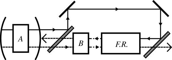
Figure 1: Scheme of the proposed all-optical feedback loop. The source mode (full line) and the driven mode (dashed line) are, respectively, horizontally and vertically polarized and are coupled within the cavity by the half-wave plate A. The source mode passes through an optically active element F.R. and the half-wave plate B, both rotating its polarization by $\pi/4$ radians, so that it finally drives the driven mode in the cavity. The output from the driven mode cannot come back into the cavity because of the action of the optically active element and of the polarized beam splitter.

3 The dynamics of the system

Before studying the dynamics of the two coupled cavity modes, it is convenient to consider the adiabatic regime where the driven mode bandwidth $\gamma_{2}=\gamma_{2}^{\prime}+\eta_{2}$ is much larger than that of the source mode. This limit will show in which way the optical feedback loop is able to inhibit the decohering effects of photon leakage. When $\gamma_{2}$ is much larger than the other parameters, the driven mode can be adiabatically eliminated so to get a master equation for the reduced density matrix of the source mode alone $\varrho$. The driven mode will always be very close to the vacuum state, so that we can expand the total density matrix $D$ as

$$D=w_{0}\otimes|0\rangle\langle 0|+w_{1}\otimes|1\rangle\langle 0|+w_{1}^{\dagger}\otimes|0\rangle\langle 1|$$

$$+w_{2}^{\prime}\otimes|1\rangle\langle 1|+w_{2}\otimes|2\rangle\langle 0|+w_{2}^{\dagger}\otimes|0\rangle\langle 2|\,,$$ (4)

where $|n\rangle$, $n=0,1,2$, are the lowest driven mode Fock states. Inserting this expression in the master equation (2), one gets a set of coupled equations for $w_{i}$, which, at lowest order in $\gamma_{2}^{-1}$, yields the following master equation for the source mode reduced density matrix $\varrho=w_{0}+w_{2}^{\prime}$

$$\dot{\varrho}(t)=\frac{\gamma_{1}}{2}\left[1+g(2+g)\frac{\gamma_{1}^{\prime}\gamma_{2}^{\prime}}{\gamma_{1}\gamma_{2}}\right]\left(2a_{1}\varrho a_{1}^{\dagger}-a_{1}^{\dagger}a_{1}\varrho-\varrho a_{1}^{\dagger}a_{1}\right)\;,$$ (5)

where $\gamma_{1}=\gamma_{1}^{\prime}+\eta_{1}$ is the total decay rate of the source mode. Equation (5) shows that, in the adiabatic limit, the dynamics of the source mode in the presence of the optical feedback loop is still described by the standard vacuum optical master equation, but with a renormalized decay rate $\gamma_{1}^{eff}=\gamma_{1}\left[1+g(2+g)\eta^{2}\right]$, where we have defined the feedback efficiency $\eta=\sqrt{\gamma_{1}^{\prime}\gamma_{2}^{\prime}/\gamma_{1}\gamma_{2}}$ (a decay rate renormalization in the adiabatic limit is already predicted in wisemil ). It is easy to see that the feedback is optimal, i.e., the effective decay rate $\gamma_{1}^{eff}$ is minimized, when the dimensionless mode conversion coupling $g=-1$, and in this case $\gamma_{1}^{eff}=\gamma_{1}\left[1-\eta^{2}\right]$. Therefore in the ideal limit of perfect feedback $\eta=1$ (i.e., no light is lost in the loop due to diffraction or absorption), when $g=-1$ and $\gamma_{2}\gg\gamma_{1}$, all-optical feedback completely freezes the source mode dynamics, that is, it realizes perfect preservation of an initial quantum state. In this ideal case, the whole source mode output is collected and converted by the all-optical loop into driven mode light, which is then efficiently converted again within the cavity into source mode light. No source mode photon is lost in the loop, and more importantly, when $g=-1$, optical feedback acts in phase, yielding a complete suppression of photon leakage. This phase-sensitive aspect of all-optical feedback cannot be achieved with electro-optical feedback. For example in pra , we have studied a direct-photodetection based electro-optical feedback loop, feeding back a photon in the cavity through atomic injection, whenever a photon is lost and detected. In this case, perfect state preservation is not achieved even in the ideal limit of unit feedback efficiency, because the fed back photon has no phase relationship with those in the cavity, and one is left with an unavoidable, even though slow, phase diffusion. This study of the adiabatic limit $\gamma_{1}/\gamma_{2}\ll 1$ shows that, with all-optical feedback, perfect state preservation is in principle possible using the scheme of Fig. 1. We now study the exact dynamics of the two coupled modes by solving the master equation (2) in order to see the performance of the scheme as a function of the feedback efficiency $\eta$ and of the adiabaticity parameter $\gamma_{1}/\gamma_{2}$. We shall consider a factorized initial condition $D(0)=\varrho_{1}(0)\otimes\varrho_{2}(0)$. It is convenient to expand the initial conditions $\varrho_{j}(0)$ using the $R$ representation qnoise

$$\varrho_{j}(0)=\frac{1}{\pi^{2}}\int\mathrm{d}^{2}\alpha_{j}\mathrm{d}^{2}\beta_{j}\;R_{j}(\beta_{j}^{*},\alpha_{j})\;|\beta_{j}\rangle\langle\alpha_{j}|\;e^{-(|\alpha_{j}|^{2}+|\beta_{j}|^{2})/2}\;,$$ (6)

where $|\alpha_{j}\rangle$ and $|\beta_{j}\rangle$ are coherent states and

$$R_{j}(\beta_{j}^{*},\alpha_{j})=\langle\beta_{j}|\varrho_{j}(0)|\alpha_{j}\rangle\;e^{(|\alpha_{j}|^{2}+|\beta_{j}|^{2})/2}$$ (7)

is the $R$ function, analytic in the two complex variables $\alpha_{j}$ and $\beta_{j}^{*}$. We are interested in the dynamics of the source mode only and, even though we do not adiabatically eliminate the driven mode, we shall always consider it more damped than the source mode. It is therefore reasonable to assume an initial vacuum state for the driven mode $\varrho_{2}(0)=|0\rangle\langle 0|$, which means $R_{2}(\beta_{2}^{*},\alpha_{2})=1$. Moreover we shall trace over the driven mode and focus on the reduced Wigner function of the source mode $W_{1}(\alpha,\alpha^{*},t)=\int\mathrm{d}^{2}\beta\,W(\alpha,\alpha^{*},\beta,\beta^{*},t)$. The time evolution of this reduced Wigner function can be determined exactly in terms of the $R$ representation of the source mode initial condition, and after some gaussian integrations one gets

$$W_{1}(\alpha,\alpha^{*},t) = \frac{2}{\pi^{3}}\int\mathrm{d}^{2}\alpha_{1}\mathrm{d}^{2}\beta_{1}\;R_{1}(\beta_{1}^{*},\alpha_{1})\;e^{-|\alpha_{1}|^{2}-|\beta_{1}|^{2}+\beta_{1}\alpha_{1}^{*}}\times$$ (8)

$$\times\;\exp\Big{[}2\big{(}\alpha-{\cal F}(t)\beta_{1}\big{)}\big{(}{\cal F}(t)\alpha_{1}^{*}-\alpha^{*}\big{)}\Big{]}\;,$$

where

$${\cal F}(t)=\frac{m+\gamma_{1}-\gamma_{2}}{2m}\mathrm{e}^{-\left(\gamma_{1}+\gamma_{2}+m\right)t/4}+\frac{m-\gamma_{1}+\gamma_{2}}{2m}\mathrm{e}^{-\left(\gamma_{1}+\gamma_{2}-m\right)t/4}$$ (9)

and $m=\sqrt{(\gamma_{1}-\gamma_{2})^{2}-4\gamma_{1}\gamma_{2}\eta^{2}(2+g)g}$. It is interesting to notice that the exact dynamics of the source mode is completely characterized by the function ${\cal F}(t)$ of (9) only. It can be shown that ${\cal F}(t)$ is always a nonincreasing function of time. In particular, in the absence of feedback ($g=0$) one has ${\cal F}(t)=\exp\left(-\gamma_{1}t/2\right)$, since the source mode is not affected by the driven mode. In the adiabatic limit, one can see from (9) that, at first order in $\gamma_{1}/\gamma_{2}$, one has ${\cal F}(t)=\exp\left(-\gamma_{1}\left(1+\eta^{2}(2+g)g\right)t/2\right)$, implying (see also section II), that in the ideal case $\eta=1$ and $g=-1$, it is ${\cal F}(t)=1$ and therefore the source mode dynamics is completely frozen.

It is instructive to apply the general expression of the time evolved Wigner function of (8) to some specific initial states of the source mode. The paradygm case for decoherence studies is the Schrödinger cat case, $\varrho_{1}(0)=|\psi(0)\rangle\langle\psi(0)|$, with

$$|\psi(0)\rangle=\frac{1}{\sqrt{2(1+e^{-2|\alpha_{0}|^{2}}\cos\varphi)}}\big{(}|\alpha_{0}\rangle+e^{i\varphi}|-\alpha_{0}\rangle\big{)}\;;$$ (10)

applying (8) one gets that the corresponding time evolution of the Wigner function is

$$W_{1}(\vec{x},t) = \frac{1}{\pi(1+e^{-2|\vec{\alpha_{0}}|^{2}}\cos\varphi)}\Big{(}e^{-2|\vec{x}-\vec{\alpha_{0}}{\cal F}(t)|^{2}}+e^{-2|\vec{x}+\vec{\alpha_{0}}{\cal F}(t)|^{2}}$$ (11)

$$+ 2e^{-2\big{(}|\vec{x}|^{2}-|\vec{\alpha_{0}}{\cal F}(t)|^{2}+|\vec{\alpha_{0}}|^{2}\big{)}}\cos\Big{(}4(\vec{x}\wedge\vec{\alpha_{0}})\cdot\hat{z}-\varphi\Big{)}\Big{)}\;,$$

where $\vec{x}=\left({\rm Re}\{\alpha\},{\rm Im}\{\alpha\},0\right)$, $\vec{\alpha_{0}}=\left({\rm Re}\{\alpha_{0}\},{\rm Im}\{\alpha_{0}\},0\right)$ and $\hat{z}=(0,0,1)$. From (11) one can see the isotropic properties of the all-optical feedback scheme studied here, since the state of the source mode depends upon the angle between $\vec{x}$ and $\vec{\alpha_{0}}$ only. The time evolution of a Schrodinger cat state with $\alpha_{0}=2{\rm i}$ and $\varphi=0$ is displayed in Fig. 2: in (a) the initial condition is shown, while in (b) and in (c) the state evolved in the presence of feedback after two decoherence times $t_{dec}=1/(2\gamma_{1}|\alpha_{0}|^{2})$ and $20t_{dec}$ are respectively shown. In (d) the state evolved after $2t_{dec}$ in the absence of feedback is instead shown. What is relevant is that, with achievable feedback parameters $g=-1$, $\eta=0.95$, and $\gamma_{1}/\gamma_{2}=10^{-3}$, one gets a very good preservation of the initial mesoscopic Schrödinger cat state ($\bar{n}=4$) after two decoherence times. With all-optical feedback, one has a decohered cat state similar to that obtained in the absence of feedback after $2t_{dec}$, only after 20 decoherence times.

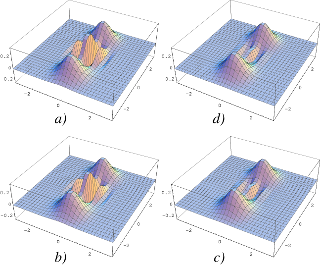
Figure 2: Time evolution of the source mode Wigner function of the cat state of equation (10) with $\alpha_{0}=2{\rm i}$, $\varphi=0$. (a) Initial Wigner function; (b) state after two decoherence times $t_{dec}$ in the presence of feedback; (c) state after $t=20t_{dec}$ in the presence of feedback. Parameter values are $g=-1$, $\eta=0.95$, and $\gamma_{1}/\gamma_{2}=10^{-3}$. (d) shows the state after $t=2t_{dec}$ in the absence of feedback ($g=0$).

Similar qualitative results are obtained with a different initial pure quantum state of the source mode, i.e., the linear superposition of Fock states $\psi(0)\rangle=\left(|2\rangle+\sqrt{2}|4\rangle\right)/\sqrt{3}$. The time evolution of the Wigner function is shown in Fig. 3, where, again, (a) shows the initial state, (b) and (c) show the state evolved in the presence of feedback after $2t_{dec}$ and after $20t_{dec}$ respectively, and (d) shows the state evolved after $2t_{dec}$ in the absence of feedback. The feedback parameters are the same as in Fig. 2. One has again a very good preservation of quantum coherence after two decoherence times.

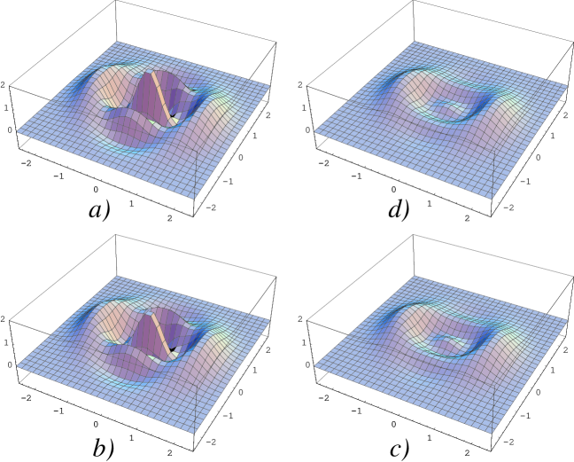
Figure 3: Time evolution of the source mode Wigner function of the linear superposition of Fock states $|\psi(0)\rangle=\left(|2\rangle+\sqrt{2}|4\rangle\right)/\sqrt{3}$. (a) Initial Wigner function; (b) state after two decoherence times $t_{dec}$ in the presence of feedback; (c) state after $t=20t_{dec}$ in the presence of feedback; (d) state after $t=2t_{dec}$ in the absence of feedback. Parameter values are the same as in Fig. 2.

A more quantitative characterization of the preservation properties of the all-optical feedback scheme is obtained from the study of the fidelity of the initial state, $F(t)={\rm Tr}\left\{\varrho_{1}(t)\varrho_{1}(0)\right\}$. Using (8) it is possible to write the fidelity of a generic initial state in terms of its $R$ representation (7) and the function ${\cal F}(t)$ as

$$F(t) = \frac{1}{\pi^{2}}\int\mathrm{d}^{2}\alpha_{1}\mathrm{d}^{2}\beta_{1}e^{-|\alpha_{1}|^{2}-|\beta_{1}|^{2}}$$

$$\times R_{1}(\beta_{1}^{*},(1-{\cal F}^{2}(t)\beta_{1}+{\cal F}(t)\alpha_{1})R_{1}(\alpha_{1}^{*},{\cal F}(t)\beta_{1})\;.$$

The time evolution of the fidelity in the case of the initial Schrödinger cat state of (10) is shown in Fig. 4. In (a) $F(t)$ is plotted for different values of the feedback efficiency $\eta$ and with fixed values for the coupling constant $g$ (the optimal choice $g=-1$ is considered) and for the ratio $\gamma_{1}/\gamma_{2}$. As expected, the preservation of the quantum state worsens for decreasing efficiencies. In (b) the effect of the timescale separation between source and driven mode is studied and $F(t)$ is plotted for different values of $\gamma_{1}/\gamma_{2}$ at fixed values for the coupling and the feedback efficiency (the optimal values $g=-1$ and $\eta=1$ are considered). We notice in particular that the decay rates ratio $\gamma_{1}/\gamma_{2}$ plays an important role and that only in the adiabatic limit $\gamma_{1}/\gamma_{2}\ll 1$ one gets a fidelity very close to one. Even in the adiabatic regime and in the ideal case (see for example the curve corresponding to $\gamma_{1}/\gamma_{2}=10^{-3}$), a finite value for $\gamma_{2}$ determines an appreciable initial slip from the condition $F(t)=1$ at small times, before the fidelity saturates to its asymptotic value.

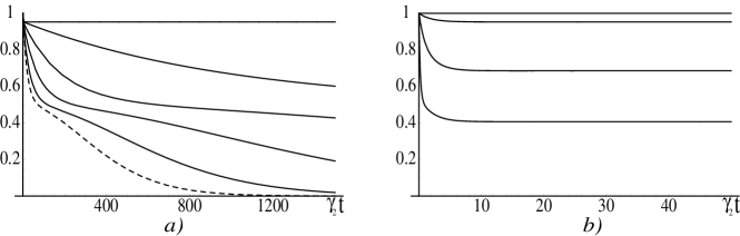
Figure 4: Time evolution of the fidelity $F(t)$ in the case of an initial Schrödinger cat state (see (10) with $\alpha_{0}=5$ and $\varphi=0$). (a) shows $F(t)$ for different values of the feedback efficiency $\eta$, with $g=-1$ and $\gamma_{1}/\gamma_{2}=10^{-3}$. From the top to the bottom: $\eta=1$, $\eta=0.99$, $\eta=0.97$, $\eta=0.95$, $\eta=0.90$; the dashed line refers to $g=0$ (absence of feedback). (b) shows $F(t)$ for different values of the decay rates ratio $\gamma_{1}/\gamma_{2}$ with $g=-1$ and $\eta=1$ kept fixed. From top to bottom: $\gamma_{1}/\gamma_{2}=0$, $\gamma_{1}/\gamma_{2}=10^{-3}$, $\gamma_{1}/\gamma_{2}=10^{-2}$, $\gamma_{1}/\gamma_{2}=10^{-1}$.

We have studied the behavior of the fidelity for a large class of initial states, as for example the linear superposition of Fock states of Fig. 3, and we have always found a behavior completely analogous to that shown in Fig. 4.

In conclusion, we have proposed an all-optical feedback scheme involving two orthogonally polarized modes in a cavity. The output light from the source mode is sent back using a Faraday isolator into the other, driven, mode and feedback is achieved by coupling the two modes within the cavity via a half-wave plate. In the adiabatic limit in which the driven mode is much more damped than the source mode, it is possible to choose the coupling constant so that in the ideal case of unit feedback efficiency one has freezing of the source mode dynamics, and therefore perfect preservation of quantum coherence. We have also shown that the protection capabilities of the scheme remain good even in the case of realistic values of the feedback efficiency.

References

- (1) Q.A. Turchette, C.J. Hood, W. Lange, H. Mabuchi, H.J. Kimble: Phys. Rev. Lett. 75, 4710 (1995).
- (2) P. Goetsch, P. Tombesi, D. Vitali: Phys. Rev. A 54, 4519 (1996).
- (3) V. Giovannetti, P. Tombesi, D. Vitali: Phys. Rev. A 60, 1549 (1999).
- (4) D. Vitali, P. Tombesi, G.J. Milburn: Phys. Rev. Lett 79, 2442 (1997).
- (5) D. Vitali, P. Tombesi, G.J. Milburn: Phys. Rev. A 58, 4930 (1998).
- (6) C.W. Gardiner: Phys. Rev. Lett 70, 2269 (1993).
- (7) H.J. Carmichael: Phys. Rev. Lett 70, 2273 (1993).
- (8) H.M. Wiseman, G.J. Milburn: Phys. Rev. A 49, 4110 (1994).
- (9) D.F. Walls, G.J. Milburn: Quantum Optics, (Springer, Berlin, 1994).
- (10) D.F. Walls, G.J. Milburn: Phys. Rev. A 31, 2403 (1985).