Disagreement between correlations of quantum mechanics and stochastic electrodynamics in the damped parametric oscillator

Abstract

Intracavity and external third order correlations in the damped nondegenerate parametric oscillator are calculated for quantum mechanics and stochastic electrodynamics (SED), a semiclassical theory. The two theories yield greatly different results, with the correlations of quantum mechanics being cubic in the system’s nonlinear coupling constant and those of SED being linear in the same constant. In particular, differences between the two theories are present in at least a mesoscopic regime. They also exist when realistic damping is included. Such differences illustrate distinctions between quantum mechanics and a hidden variable theory for continuous variables.

I Introduction

Local hidden variable theories have been extensively compared to quantum mechanics over the last seventy or so years [1, 2, 3]. Most comparisons between the two have investigated whether or not quantum mechanics is equivalent to a local hidden variable theory. Much evidence indicates that it is not. Many results in quantum mechanics have been found that are incompatible with all local hidden variable theories [2, 3, 4, 5, 6, 7]. Most of these results have involved idealized undamped systems. However, all experimental systems encounter damping. Thus, it is interesting (and more realistic) to compare quantum mechanics and local hidden variable theories in damped systems [5]. This paper compares quantum mechanics and one local hidden variable theory (SED) in such a system.

One of the earliest works comparing local hidden variable theories to quantum mechanics was Bell’s theorem [2]. It demonstrates that quantum mechanics is incompatible with all local hidden variable theories at a statistical level. It does so by deriving an upper bound on a function of two particle correlations for all local hidden variable theories, which quantum mechanics exceeds. Extensions of it have been formulated for large angular momentum and particle number systems [5, 6]. These extensions demonstrate nonclassical behavior in a regime usually regarded as being purely classical. Greenberger, Horne and Zeilinger (GHZ) [4] have also extended Bell’s work, differentiating quantum mechanics from all local hidden variable theories for single, as opposed to ensemble, measurements. The three particle GHZ theorem has an “all or nothing” quality and distinguishes between local hidden variable theories and quantum mechanics in a single experimental run, once three basic correlations are established.

Comparisons between quantum mechanics and local hidden variable theories have also been made using continuous variables (which are discretized in formulating the comparison), such as quadrature phase amplitudes [7] and there is currently much interest in this area. For quadrature phase amplitude measurements, these comparisons can have detector efficiencies of in excess of 99% [9]. They also tend to relate more strongly to Einstein, Podolsky and Rosen’s original EPR paradox [1] than earlier discrete variable ones. Indeed, the EPR paradox has been experimentally demonstrated using quadrature phase amplitudes [8]. Additionally, quantum teleportation has been achieved using quadrature phase amplitudes [10] further demonstrating the utility of continuous variables.

One commonly used local hidden variable theory is stochastic electrodynamics (SED) [11, 12]. Some authors have proposed it as an alternative to quantum mechanics [11, 13]. Furthermore, a semiclassical approach equivalent to it [14] is also commonly used in parametric oscillator calculations [15]. SED consists of adding Gaussian white noise to classical electrodynamics. It is equivalent to truncating third order derivative terms in the quantum mechanical Moyal equation, a commonly used approximation [16]. Such terms are often negligible and thus SED reproduces many results of quantum mechanics [14, 15]. However, it cannot violate Bell inequalities for quadrature phase amplitude measurements, and is thus distinct from quantum mechanics [7]. Various authors have explicitly shown differences between SED and quantum mechanics [17, 18, 19]. In particular, it has been shown that the two theories predict different transient third order correlations for the undamped nondegenerate parametric oscillator [17]. It has also been shown that they predict different macroscopic quadrature phase amplitude correlations in the damped nondegenerate parametric oscillator in the steady state [19].

In general, differences between quantum mechanics and local hidden variable theories are reduced or eliminated by damping [20]. Furthermore, damping is a significant element of many realistic systems. It is thus important to consider its effects on differences between quantum mechanics and local hidden variable theories such as SED. However, all but a few of the comparisons between the quantum mechanics and local hidden variable theories referenced above have involved undamped systems. They are thus idealized in this respect. In contrast, damping is included in the calculatons in this paper. It is included to consider a theoretical model which is as realistic as possible and also to determine the sensitivity of differences between quantum mechanics and SED to its presence.

This paper extends a previous comparison between quantum mechanics and SED in the nondegenerate parametric oscillator [17]. In particular, it contrasts both intracavity and external moments of the two theories’ in the same system with damping included. Expressions from both theories are compared for the intracavity moment $\langle\Delta X_{1}(\tau)\Delta(X_{2}(\tau)\Delta X_{3}(\tau)\rangle$, where $\Delta X_{i}(\tau)=X_{i}(\tau)-\langle X_{i}(\tau)\rangle$, for $i=1,2,3$, $X_{i}(\tau)$ is quadrature phase amplitude, the subscripts represent different radiation modes and $\tau$ is a scaled time variable. A comparison is also made for an analogous external moment. Both analytic iterative and numerical techniques are used to calculate moments. The results produced by these techniques show that the intracavity and external moments differ greatly between the two theories. In particular, the analytic method shows that the moments of quantum mechanics are cubic in the system’s nonlinear coupling constant to leading order whilst those of SED are linear. The two theories are compared over a range of nonlinear coupling constant, damping and average initial pump photon number values. The results of these comparisons show a number of qualitative trends. Most importantly, quantum mechanics and SED differ in the situations considered with the largest particle number and damping to nonlinear coupling ratios, although the differences are reduced in relative size.

Stochastic techniques are used to obtain results both for quantum mechanics and SED. The positive-P coherent state representation [21] is used to calculate quantum mechanical predictions. It is particularly well suited to the calculation of quantum dynamics in damped quantum optical systems when nonclassical behavior is present. It is able to handle arbitrarily large photon numbers. It converges quickly (in the sense of sampling error) when systems’ dimensionless nonlinearities are relatively small, as is the case with nonlinear optical experiments. By contrast, the method used for SED calculations corresponds to commonly used approaches in quantum optics, where the field is treated as a semiclassical object surrounded by (classical) vacuum fluctuations. Both methods are used to generate analytic predictions and are also numerically simulated.

II Quantum mechanics

This paper considers an idealized nondegenerate parametric oscillator, resonant at three frequencies $\omega_{1}\>{\rm and}\>\>\>\omega_{2}$ (signal and idler frequencies) and $\omega_{3}\>=\omega_{1}+\omega_{2}$ (pump frequency). It contains a nonlinear medium that couples the modes and converts higher energy pump photons into lower energy signal and idler ones. The system’s interaction Hamiltonian, including linear losses, is given by

$$\hat{H}=i\hbar G({\hat{a}}^{{\dagger}}_{1}{\hat{a}}^{{\dagger}}_{2}{\hat{a}}_{3}-{\hat{a}}_{1}{\hat{a}}_{2}{\hat{a}}^{{\dagger}}_{3})+\sum^{3}_{i=1}{\hat{\Gamma}}_{i}{\hat{a}}_{i}^{{\dagger}}+{\hat{\Gamma}}_{i}^{{\dagger}}{\hat{a}}_{i},$$ (1)

where ${\hat{a}}_{i}^{{\dagger}}\>{\rm and}\>{\hat{a}}_{i}$ are creation and annihilation operators for oscillator modes, ${\hat{\Gamma}}^{{\dagger}}_{i}\>{\rm and}\>{\hat{\Gamma}}_{i}$ are environment mode operators and G is a nonlinear interaction strength constant. Initially, the system has a coherent state in the pump mode, and vacuum states in the signal and idler modes.

A number of quasiprobability representations exist to describe quantum states, the most famous being the Glauber-Sudarshan representation[22]. It is produced by decomposing quantum density operators using a diagonal coherent state basis. Thus,

$${\hat{\rho}}=\int d\alpha^{2}P(\alpha,\alpha^{*})|\alpha\rangle\langle\alpha|,$$ (2)

where ${\hat{\rho}}$ is a density operator and $P(\alpha,\alpha^{*})$ is the Glauber-Sudarshan representation. The Glauber-Sudarshan representation can be negative and is hence not a strict probability density function. A more recent representation is the positive-P representation [21] which is an actual probability density function over an off-diagonal coherent state basis. It further differs from the Glauber-Sudarshan representation by using a phase space of doubled dimension. The positive-P variables $\{\alpha_{i},\alpha^{+}_{i}\}$, where $i$ is a positive integer, are analogous to complex field amplitudes, with $\alpha_{i}$ and $\alpha^{+}_{i}$ describing a particular radiation mode. However, $\{\alpha_{i}\}$ and $\{\alpha^{+}_{i}\}$ are independent and hence $\alpha_{i}\neq(\alpha^{+}_{i})^{*}$, though their averages are complex conjugate and thus $\langle\alpha_{i}\rangle=\langle\alpha_{i}^{+}\rangle^{*}$. Variable averages are equal to normally ordered quantum averages once the substitutions $\alpha_{i}\rightarrow{\hat{a}}_{i}$ and $\alpha_{i}^{+}\rightarrow{\hat{a}}_{i}^{{\dagger}}$ are made. For example, $\langle\alpha_{1}\alpha_{1}^{+}\rangle=\langle{\hat{a}}_{1}^{{\dagger}}{\hat{a}}_{1}\rangle_{\rho}$, where $\langle\hat{O}\rangle_{\rho}$ denotes $Tr(\hat{\rho}\hat{O})$, as usual in quantum mechanics.

Stochastic equations of motion for positive-P variables for the damped nondegenerate parametric oscillator are, in terms of $\tau$ (time scaled by $\Gamma$, a typical damping constant with units of inverse time),

$$\frac{d\alpha_{1}}{d\tau} = -\gamma_{1}\alpha_{1}+g\alpha_{2}^{+}\alpha_{3}+\sqrt{g\alpha_{3}}\xi_{1}$$ (3)

$$\frac{d\alpha_{1}^{+}}{d\tau} = -\gamma_{1}\alpha_{1}^{+}+g\alpha_{2}\alpha_{3}^{+}+\sqrt{g\alpha_{3}^{+}}\xi_{1}^{+}$$ (4)

$$\frac{d\alpha_{2}}{d\tau} = -\gamma_{2}\alpha_{2}+g\alpha_{1}^{+}\alpha_{3}+\sqrt{g\alpha_{3}}\xi_{2}$$ (5)

$$\frac{d\alpha_{2}^{+}}{d\tau} = -\gamma_{2}\alpha_{2}^{+}+g\alpha_{1}\alpha_{3}^{+}+\sqrt{g\alpha_{3}^{+}}\xi_{2}^{+}$$ (6)

$$\frac{d\alpha_{3}}{d\tau} = -\gamma_{3}\alpha_{3}-g\alpha_{1}\alpha_{2}$$ (7)

$$\frac{d\alpha_{3}^{+}}{d\tau} = -\gamma_{3}\alpha_{3}^{+}-g\alpha_{1}^{+}\alpha_{2}^{+}.$$ (8)

Here $\xi_{1},\>\xi_{2},\>\xi^{+}_{1}{\rm\>and\>}\xi^{+}_{2}$ are complex Gaussian white noises with the following correlations

$$\langle\xi_{i}(\tau_{1})\xi_{j}(\tau_{2})\rangle = \delta_{3-i,j}\delta(\tau_{1}-\tau_{2})$$ (9)

$$\langle\xi_{i}^{+}(\tau_{1})\xi_{j}^{+}(\tau_{2})\rangle = \delta_{3-i,j}\delta(\tau_{1}-\tau_{2})$$ (10)

$$\langle\xi_{i}^{+}(\tau_{1})\xi_{j}(\tau_{2})\rangle = 0,$$ (11)

where $i,j=1,2$. In Eq. (3), $\gamma_{i}=\Gamma_{i}/\Gamma$, where $\Gamma_{i}$ is a damping constant for mode $i$ with units of inverse time, $g=G/\Gamma$ and $\tau=\Gamma t$. It is assumed that G, $\Gamma_{i}$ and $\Gamma$ are real. Initial conditions are $\alpha_{1}(0)=0,\>\alpha_{2}(0)=0\>{\rm and}\>\alpha_{3}(0)=\epsilon$. It is noted that Eq. (3) is only valid when boundary terms in phase space can be neglected. These are asymptotically small in the limit of short times or large damping ratios [23].

Eq. 3 is solved using an analytic iterative method. This method treats damping terms exactly, and noise and nonlinear terms iteratively. It involves, firstly, rewriting the equations forming Eq. (3) as $\dot{\alpha}_{i}=-\gamma_{i}\alpha_{i}+f_{i}(\{\alpha_{j},\alpha^{+}_{j}\},\tau)$ or $\dot{\alpha}_{i}^{+}=-\gamma_{i}\alpha_{i}^{+}+f^{+}_{i}(\{\alpha_{j},\alpha^{+}_{j}\},\tau)$, where $i,j=1,2,3$. Successively higher order approximations for $\{\alpha_{i}(\tau),\alpha_{i}^{+}(\tau)\}$ are then found using increasingly better approximations for $f_{i}$ and $f_{i}^{+}$. Thus, $(m+1)^{th}$ order terms are given by

$$\alpha_{i}^{(m+1)}(\tau) = \alpha_{i}^{(0)}(\tau)+\int_{\tau_{1}=0}^{\tau_{1}=\tau}d\tau_{1}\exp[{\gamma_{i}(\tau_{1}-\tau)}]f_{i}(\{\alpha^{(m)}_{j},\alpha^{+\>(m)}_{j}\},\tau_{1})$$ (12)

$$\alpha_{i}^{+\>(m+1)}(\tau) = \alpha_{i}^{+\>(0)}(\tau)+\int_{\tau_{1}=0}^{\tau_{1}=\tau}d\tau_{1}\exp[{\gamma_{i}(\tau_{1}-\tau)}]f^{+}_{i}(\{\alpha^{(m)}_{j},\alpha^{+\>(m)}_{j}\},\tau_{1}),$$ (13)

where $\alpha_{k}^{(0)}(\tau)=\alpha_{k}(\tau=0)\exp(-\gamma_{k}\tau)$ and $\alpha_{k}^{(0)\>+}(\tau)=\alpha_{k}^{(0)}(\tau)^{*}$ where $k=1,2,3$. For example,

$$\alpha_{1}^{(m+1)}(\tau)=\alpha_{1}^{(0)}(\tau)+\int_{\tau_{1}=0}^{\tau_{1}=\tau}d\tau_{1}\exp[{\gamma_{1}(\tau_{1}-\tau)}]\bigl{(}g\alpha_{2}^{+\>(m)}(\tau_{1})\alpha_{3}^{(m)}(\tau_{1})+\sqrt{g\alpha_{3}^{(m)}(\tau_{1})}\xi_{1}(\tau_{1})\bigr{)}$$ (14)

and first order approximations are

$$\alpha_{i}^{(1)}(\tau) = \int_{\tau_{i}=0}^{\tau_{i}=\tau}d\tau_{i}\exp[\gamma_{i}(\tau_{i}-\tau)]\sqrt{g\epsilon}\exp(-\frac{\gamma_{i}\tau_{i}}{2})\xi_{i}(\tau_{1})$$ (15)

$$\alpha_{3}^{(1)}(\tau) = \epsilon\exp(-\gamma_{3}\tau)$$ (16)

$$\alpha_{i}^{+\>(1)}(\tau) = \int_{\tau_{i}=0}^{\tau_{i}=\tau}d\tau_{i}\exp[\gamma_{i}(\tau_{i}-\tau)]\sqrt{g\epsilon^{*}}\exp(-\frac{\gamma_{i}\tau_{i}}{2})\xi_{i}^{+}(\tau_{1})$$ (17)

$$\alpha_{3}^{+\>(1)}(\tau) = \epsilon^{*}\exp(-\gamma_{3}\tau),$$ (18)

where $i=1,2$.

III Stochastic diagrams

The iterative method of the previous section can be used, in conjunction with stochastic diagrams, to readily produce analytic approximations for the intracavity moments of quantum mechanics considered in this paper. Stochastic diagrams [24] are schematic representations of the combinatoric parts of an iterative process. They clearly lay out all terms produced by different orders of iteration. Fundamental stochastic diagrams appear as one of three classes. Those associated with initial conditions appear as straight lines, those with noise terms as straight lines with a cross at their end and those with nonlinear terms as straight lines containing a fork, as shown in Fig. 1(a)-(c). Higher order iterative terms are represented by stochastic diagrams using either combinations of the three basic classes. For example, one of the iterative terms in $\alpha_{1}^{(2)}(\tau)$ is

$$\int_{\tau_{1}=0}^{\tau_{1}=\tau}d\tau_{1}\exp[\gamma_{1}(\tau_{1}-\tau)]g\alpha_{3}^{(0)}(\tau_{1})\int_{\tau_{2}=0}^{\tau_{2}=\tau_{1}}d\tau_{2}\exp[\gamma_{2}(\tau_{2}-\tau_{1})]\sqrt{g\epsilon^{*}}\exp(-\frac{\gamma_{2}\tau_{2}}{2})\xi_{2}^{+}(\tau_{2}).$$

It combines all three basic classes and is represented by the stochastic diagram in Fig. 1(d). All iterative terms can be represented by stochastic diagrams.

Stochastic diagrams can also be used to determine the orders of iterative terms. In particular, they can be used to determine the orders of such terms in the system’s nonlinear coupling constant g. This paper focuses on the order of terms in this constant. For quantum mechanics, initial value iterative terms are $O(g^{0})$, noise iterative terms $O(g^{1/2})$ and nonlinear iterative terms $O(g)$. Hence, lines in stochastic diagrams count as order zero, crosses as order 1/2 and vertices as order 1. A term’s order is simply found by considering its stochastic diagram and adding a half to its order for every cross and one for every vertex. For example, the term represented in Fig. 1(d) has one vertex and one cross and thus is $O(g^{\frac{3}{2}})$. A notation that denotes the order in g of a term by a superscript [n] is used in this section.

Stochastic diagrams are now used to determine the intracavity moments of quantum mechanics considered in this paper. Consider all eight moments of the form $\langle\Delta{\cal A}_{1}(\tau)\Delta{\cal A}_{2}(\tau)\Delta{\cal A}_{3}(\tau)\rangle$, where $\Delta{\rm{\cal A}_{i}}(\tau)={\cal A}_{i}(\tau)-\langle{\cal A}_{i}(\tau)\rangle$ and ${\cal A}_{i}(\tau)$ is either ${\hat{a}}_{i}$ or ${\hat{a}}^{{\dagger}}_{i}$. These are equal to the positive-P variable moments which replace ${\hat{a}}_{i}$ and $\hat{a}_{i}^{{\dagger}}$ by $\alpha_{i}(\tau)$ and $\alpha_{i}^{+}(\tau)$ respectively. Now, consider the equations that constitute Eq. (3). Their forms do not change when they are expressed in terms of $-\alpha_{i}(\tau),-\alpha_{i}^{+}(\tau),\alpha_{3}(\tau)$ and $\alpha_{3}^{+}(\tau)$, where $i=1,2$. From this, it follows that $\langle{\cal A}_{i}(\tau)\rangle=\langle-{\cal A}_{i}(\tau)\rangle$ and hence $\langle\alpha_{i}(\tau)\rangle=\langle\alpha_{i}^{+}(\tau)\rangle=0$, where again $i=1,2$. Thus, $\langle\Delta{\cal A}_{1}(\tau)\Delta{\cal A}_{2}(\tau)\Delta{\cal A}_{3}(\tau)\rangle$ can be simplified to $\langle{\cal A}_{1}(\tau){\cal A}_{2}(\tau)\Delta{\cal A}_{3}(\tau)\rangle$.

An approximate expression for $\langle{\cal A}_{1}(\tau){\cal A}_{2}(\tau)\Delta{\cal A}_{3}(\tau)\rangle$ is now obtained using the iterative method in Section II (and stochastic diagrams). This method can be used to produce power series expressions in $g$ for the positive-P variables. These expressions can then be used to generate power series expressions in $g$ for the moments of the form $\langle{\cal A}_{1}(\tau){\cal A}_{2}(\tau)\Delta{\cal A}_{3}(\tau)\rangle$. As $g\ll 1$ in realistic systems, these power series expressions can be approximated by their lowest order nonzero terms.

Figs 2 (a) and (b) show the stochastic diagrams required to determine the moments of the form $\langle{\cal A}_{1}(\tau){\cal A}_{2}(\tau)\Delta{\cal A}_{3}(\tau)\rangle$. Naively, it might be thought that the lowest order nonzero terms from ${\cal A}_{1}(\tau),\>{\cal A}_{2}(\tau)\>{\rm and}\>\Delta\>{\cal A}_{3}(\tau)$ simply need to be multiplied together and the average of the subsequent product determined to calculate the lowest order nonzero term in $\langle{\cal A}_{1}(\tau)\>{\cal A}_{2}(\tau)\Delta\>{\cal A}_{3}(\tau)\rangle$. This is not always true. Sometimes, ${\cal A}_{1}(\tau),\>{\cal A}_{2}(\tau)\>{\rm and}\>\Delta\>{\cal A}_{3}(\tau)$ are not necessarily zero and yet $\langle{\cal A}_{1}(\tau){\cal A}_{2}(\tau)\Delta{\cal A}_{3}(\tau)\rangle$ is zero. For example, the lowest order nonzero terms for the positive-P variables in $\langle\alpha_{1}(\tau)\alpha_{2}(\tau)\Delta\alpha_{3}^{+}(\tau)\rangle$ are

$$\alpha_{i}^{[1/2]}(\tau)=\int_{\tau_{i}=0}^{\tau_{i}=\tau}d\tau_{i}\exp[\gamma_{i}(\tau_{i}-\tau)]\sqrt{g\epsilon}\exp(-\frac{\gamma_{i}\tau_{i}}{2})\xi_{i}(\tau_{i}),$$ (19)

where $i=1,2$ and

$$\Delta\alpha_{3}^{+\>[2]}(\tau) = \int_{\tau_{3}=0}^{\tau_{3}=\tau}d\tau_{3}\exp[\gamma_{3}(\tau_{3}-\tau)]g\int_{\tau_{4}=0}^{\tau_{4}=\tau_{3}}d\tau_{4}\exp[\gamma_{1}(\tau_{4}-\tau_{3})]\sqrt{g\epsilon^{*}}\exp(-\frac{\gamma_{1}\tau_{4}}{2})\xi_{1}^{+}(\tau_{4})$$ (23)

$$\int_{\tau_{5}=0}^{\tau_{5}=\tau_{3}}d\tau_{5}\exp[\gamma_{2}(\tau_{5}-\tau_{3})]\sqrt{g\epsilon^{*}}\exp(-\frac{\gamma_{2}\tau_{5}}{2})\xi_{2}^{+}(\tau_{5})$$

$$-\bigl{\langle}\int_{\tau_{3}=0}^{\tau_{3}=\tau}d\tau_{3}\exp[\gamma_{3}(\tau_{3}-\tau)]g\int_{\tau_{4}=0}^{\tau_{4}=\tau_{3}}d\tau_{4}\exp[\gamma_{1}(\tau_{4}-\tau_{3})]\sqrt{g\epsilon^{*}}\exp(-\frac{\gamma_{1}\tau_{4}}{2})\xi_{1}^{+}(\tau_{4})$$

$$\int_{\tau_{5}=0}^{\tau_{5}=\tau_{3}}d\tau_{5}\exp[\gamma_{2}(\tau_{5}-\tau_{3})]\sqrt{g\epsilon^{*}}\exp(-\frac{\gamma_{2}\tau_{5}}{2})\xi_{2}^{+}(\tau_{5})\bigr{\rangle}.$$

However, the average of their product is zero as

$$\bigl{\langle}\alpha_{1}^{[1/2]}(\tau)\alpha_{2}^{[1/2]}(\tau)\Delta\alpha_{3}^{+\>[2]}(\tau)\bigr{\rangle}$$ (24)

$$= g^{3}\epsilon\epsilon^{*}\int_{\tau_{1}=0}^{\tau_{1}=\tau}\int_{\tau_{2}=0}^{\tau_{2}=\tau}\int_{\tau_{3}=0}^{\tau_{3}=\tau}\int_{\tau_{4}=0}^{\tau_{4}=\tau_{3}}\int_{\tau_{5}=0}^{\tau_{5}=\tau_{3}}d\tau_{1}d\tau_{2}d\tau_{3}d\tau_{4}d\tau_{5}$$ (27)

$$\exp[\gamma_{1}(\tau_{1}-\tau)]\exp(-\frac{\gamma_{1}\tau_{1}}{2})\exp[\gamma_{2}(\tau_{2}-\tau)]\exp(-\frac{\gamma_{2}\tau_{2}}{2})\exp[\gamma_{3}(\tau_{3}-\tau)]\exp[\gamma_{1}(\tau_{4}-\tau_{3})]\exp(-\frac{\gamma_{1}\tau_{4}}{2})$$

$$\exp[\gamma_{5}(\tau_{5}-\tau_{3})]\exp(-\frac{\gamma_{2}\tau_{5}}{2})\bigl{(}\langle\xi_{1}(\tau_{1})\xi_{2}(\tau_{2})\xi_{1}^{+}(\tau_{4})\xi_{2}^{+}(\tau_{5})\rangle-\langle\xi_{1}(\tau_{1})\xi_{2}(\tau_{2})\rangle\>\langle\xi_{1}^{+}(\tau_{4})\xi_{2}^{+}(\tau_{5})\rangle\bigl{)}$$

and

$$\langle\xi_{1}(\tau_{1})\xi_{2}(\tau_{2})\xi_{1}^{+}(\tau_{4})\xi_{2}^{+}(\tau_{5})\rangle=\langle\xi_{1}(\tau_{1})\xi_{2}(\tau_{2})\rangle\>\langle\xi_{1}^{+}(\tau_{4})\xi_{2}^{+}(\tau_{5})\rangle.$$ (28)

Thus, the two noise terms cancel each other and the right hand side of Eq. (28) is zero. Taking such a consideration into account, the moments of the form $\langle{\cal A}_{1}(\tau){\cal A}_{2}(\tau)\Delta{\cal A}_{3}(\tau)\rangle$ are determined by carefully considering the lowest order nonzero terms of their constituent positive-P variables and then finding the average of these variables’ products.

Consider Fig. (2)(a), which contains the lowest order stochastic diagrams for $\alpha_{i}(\tau)$ and $\alpha_{i}^{+}(\tau)$, where $i=1,2$. The first diagram in it represents the initial value terms $\alpha_{i}^{(0)}(\tau)$ and $\alpha_{i}^{(0)\>+}(\tau)$, which are zero and do not contribute to any moments. The second represents terms containing $\xi_{1},\xi_{1}^{+},\xi_{2}$ or $\xi_{2}^{+}$, which are not necessarily zero and thus may contribute to moments. Fig. 2(b) contains the lowest order stochastic diagrams for $\alpha_{3}(\tau)$ and $\alpha_{3}^{+}(\tau)$. In it, all terms represented by stochastic diagrams containing initial value lines are zero except for the $O(g^{0})$ ones. This is so as these terms contain either $\alpha_{i}^{(0)}(\tau)\>{\rm or}\>\alpha_{i}^{+\>(0)}(\tau)$, where $i=1,2$, which are both zero. In addition, all $O(g^{0})$ terms represented by stochastic diagrams in Fig. 2(b) are canceled out by other $O(g^{0})$ terms. This occurs because $\Delta{\cal A}_{3}(\tau)$ appears in the moments considered. Its two components, ${\cal A}_{3}(\tau)$ and $\langle{\cal A}_{3}(\tau)\rangle$, contain the same $O(g^{0})$ term and hence their $O(g^{0})$ terms cancel each other. It follows that the only remaining stochastic diagram in Fig. 2(b), which represents the $O(g^{2})$ term containing two noise components, denotes the lowest order term in $\Delta{\cal A}_{3}(\tau)$ that is not necessarily zero.

The lowest order nonzero terms determined above are now used to calculate $\langle\alpha_{1}(\tau)\alpha_{2}(\tau)\Delta\alpha_{3}(\tau)\rangle$. The lowest order contribution to $\Delta\alpha_{3}(\tau)$ that is not necessarily zero $\Delta\alpha_{3\>{\rm lowest}}(\tau)$ is

$$\Delta\alpha_{3\>{\rm lowest}}(\tau) = \int_{\tau_{3}=0}^{\tau_{3}=\tau}d\tau_{3}\exp[\gamma_{3}(\tau_{3}-\tau)]g\int_{\tau_{4}=0}^{\tau_{4}=\tau_{3}}d\tau_{4}\exp[\gamma_{1}(\tau_{4}-\tau_{3})]\sqrt{g\epsilon}\exp(-\frac{\gamma_{1}\tau_{4}}{2})\xi_{1}(\tau_{4})$$ (32)

$$\int_{\tau_{5}=0}^{\tau_{5}=\tau_{3}}d\tau_{5}\exp[\gamma_{2}(\tau_{5}-\tau_{3})]\sqrt{g\epsilon}\exp(-\frac{\gamma_{2}\tau_{5}}{2})\xi_{2}(\tau_{5})$$

$$-\bigl{\langle}\int_{\tau_{3}=0}^{\tau_{3}=\tau}d\tau_{3}\exp[\gamma_{3}(\tau_{3}-\tau)]g\int_{\tau_{4}=0}^{\tau_{4}=\tau_{3}}d\tau_{4}\exp[\gamma_{1}(\tau_{4}-\tau_{3})]\sqrt{g\epsilon}\exp(-\frac{\gamma_{1}\tau_{4}}{2})\xi_{1}(\tau_{4})$$

$$\int_{\tau_{5}=0}^{\tau_{5}=\tau_{3}}d\tau_{5}\exp[\gamma_{2}(\tau_{5}-\tau_{3})]\sqrt{g\epsilon}\exp(-\frac{\gamma_{2}\tau_{5}}{2})\xi_{2}(\tau_{5})\bigr{\rangle}.$$

When $\gamma_{1}=\gamma_{2}=\gamma_{3}=\gamma$, the average of the product of $\Delta\alpha_{3\>{\rm lowest}}(\tau)$ and the lowest order nonzero terms in $\alpha_{1}(\tau)$ and $\alpha_{2}(\tau)$ is approximately equal to $\langle\alpha_{1}(\tau)\alpha_{2}(\tau)\Delta\alpha_{3}(\tau)\rangle$ when $g\ll 1$ and thus

$$\langle\alpha_{1}(\tau)\alpha_{2}(\tau)\Delta\alpha_{3}(\tau)\rangle \simeq -\frac{\epsilon^{2}g^{3}\exp[-3\gamma\tau]}{\gamma^{2}}\times\bigl{[}\frac{\exp[\gamma\tau]}{\gamma}-2\tau-\frac{\exp[-\gamma\tau]}{\gamma}\bigr{]}.$$ (33)

As daggered positive-P variables are complex conjugate to undaggered ones on average, $\langle\alpha_{1}^{+}(\tau)\alpha_{2}^{+}(\tau)\Delta\alpha_{3}^{+}(\tau)\rangle=\langle\alpha_{1}(\tau)\alpha_{2}(\tau)\Delta\alpha_{3}(\tau)\rangle^{*}$. The other six moments of the form $\langle{\cal A}_{1}(\tau){\cal A}_{2}(\tau)\Delta{\cal A}_{3}(\tau)\rangle$ are zero to $O(g^{3})$. As does $\langle\alpha_{1}(\tau)\alpha_{2}(\tau)\Delta\alpha_{3}^{+}(\tau)\rangle$, they all have two $O(g^{3})$ terms that cancel each other. To explain such behaviour in general, the following argument is given. These other six moments can be rewritten as

$$\langle{\cal A}_{1}(\tau){\cal A}_{2}(\tau){\cal A}_{3}(\tau)\rangle-\langle{\cal A}_{1}(\tau){\cal A}_{2}(\tau)\rangle\langle{\cal A}_{3}(\tau)\rangle,$$ (34)

where it is understood that the moments in which ${\cal A}_{1}(\tau)=\alpha_{1}(\tau),{\cal A}_{2}(\tau)=\alpha_{2}(\tau),{\cal A}_{3}(\tau)=\alpha_{3}(\tau)$ and ${\cal A}_{1}(\tau)=\alpha_{1}^{+}(\tau),{\cal A}_{2}(\tau)=\alpha_{2}^{+}(\tau),{\cal A}_{3}(\tau)=\alpha_{3}^{+}(\tau)$ are excluded. All $O(g^{3})$ terms in the six moments of the form $\langle{\cal A}_{1}(\tau){\cal A}_{2}(\tau){\cal A}_{3}(\tau)\rangle$ under consideration contain noises in one of the following three forms, $\bigl{\langle}\xi_{1}(\tau_{a})\xi_{2}(\tau_{b})\xi_{1}^{{\dagger}}(\tau_{c})\xi_{2}^{{\dagger}}(\tau_{d})\bigr{\rangle}$, $\bigl{\langle}\xi_{i}(\tau_{a})\xi_{3-i}^{{\dagger}}(\tau_{b})\xi_{i}(\tau_{c})\xi_{3-i}(\tau_{d})\bigr{\rangle}$ and $\bigl{\langle}\xi_{i}^{{\dagger}}(\tau_{a})\xi_{3-i}(\tau_{b})\xi_{i}^{{\dagger}}(\tau_{c})\xi_{3-i}^{{\dagger}}(\tau_{d})\bigr{\rangle}$, where $i=1,2$ and time arguments are dummy variables. All $O(g^{3})$ terms in the six moments of the form $\langle{\cal A}_{1}(\tau){\cal A}_{2}(\tau)\rangle\langle{\cal A}_{3}(\tau)\rangle$ under consideration contain the same noises as their corresponding $\langle{\cal A}_{1}(\tau){\cal A}_{2}(\tau){\cal A}_{3}(\tau)\rangle$ term. However, in these terms of the form $\langle{\cal A}_{1}(\tau){\cal A}_{2}(\tau)\rangle\langle{\cal A}_{3}(\tau)\rangle$ four noise averages from corresponding terms of the form $\langle{\cal A}_{1}(\tau){\cal A}_{2}(\tau){\cal A}_{3}(\tau)\rangle$ are split into the product of two averages of two noises. For example, $\langle\alpha_{1}(\tau)\alpha_{2}(\tau)\alpha_{3}^{+}(\tau)\rangle$ contains noises in the form $\langle\xi_{1}(\tau_{a})\xi_{2}(\tau_{b})\xi_{1}^{+}(\tau_{c})\xi_{2}^{+}(\tau_{d})\rangle$ whilst $\langle\alpha_{1}(\tau)\alpha_{2}(\tau)\rangle\langle\alpha_{3}^{+}(\tau)\rangle$ contains them in the form $\langle\xi_{1}(\tau_{a})\xi_{2}(\tau_{b})\rangle\langle\xi_{1}^{+}(\tau_{c})\xi_{2}^{+}(\tau_{d})\rangle$. Using the formula

$$\bigl{\langle}\xi_{1}(\tau_{a})\xi_{2}(\tau_{b})\xi_{3}(\tau_{c})\xi_{4}(\tau_{d})\bigr{\rangle} = \>\>\>\bigl{\langle}\xi_{1}(\tau_{a})\xi_{2}(\tau_{b})\bigr{\rangle}\bigl{\langle}\xi_{3}(\tau_{c})\xi_{4}(\tau_{d})\bigr{\rangle}$$ (37)

$$+\bigl{\langle}\xi_{1}(\tau_{a})\xi_{3}(\tau_{c})\bigr{\rangle}\>\bigl{\langle}\xi_{2}(\tau_{b})\xi_{4}(\tau_{d})\bigr{\rangle}$$

$$+\bigl{\langle}\xi_{1}(\tau_{a})\xi_{4}(\tau_{d})\bigr{\rangle}\>\bigl{\langle}\xi_{2}(\tau_{b})\xi_{3}(\tau_{c})\bigr{\rangle}$$

it can be shown that noise expressions in moments of the form $\langle{\cal A}_{1}(\tau){\cal A}_{2}(\tau){\cal A}_{3}(\tau)\rangle$ under consideration factorize. In particular, they reduce to the noise expression in the six corresponding term of the form $\langle{\cal A}_{1}(\tau){\cal A}_{2}(\tau)\rangle\langle{\cal A}_{3}(\tau)\rangle$. It follows that cancellation occurs between the $O(g^{3})$ terms in corresponding moments of the form $\langle{\cal A}_{1}(\tau){\cal A}_{2}(\tau){\cal A}_{3}(\tau)\rangle$ and $\langle{\cal A}_{1}(\tau){\cal A}_{2}(\tau)\rangle\langle{\cal A}_{3}(\tau)\rangle$ under consideration as the two terms are identical. Consequently, all six moments under consideration are $O(g^{4})$. They are also typically much smaller than the two $O(g^{3})$ moments, $\langle\alpha_{1}(\tau)\alpha_{2}(\tau)\Delta\alpha_{3}(\tau)\rangle$ and $\langle\alpha_{1}^{+}(\tau)\alpha_{2}^{+}(\tau)\Delta\alpha_{3}^{+}(\tau)\rangle$, as $g\ll 1$ for realistic systems. To be precise, as all moments are complex quantities, the magnitudes of $\langle\alpha_{1}(\tau)\alpha_{2}(\tau)\Delta\alpha_{3}(\tau)\rangle$ and $\langle\alpha_{1}^{+}(\tau)\alpha_{2}^{+}(\tau)\Delta\alpha_{3}^{+}(\tau)\rangle$ are much larger than the magnitudes of the other six moments.

The above results are now more closely related to experiments by considering quadrature phase amplitudes $X_{i,\theta_{i}}(\tau)$. In particular, calculations are performed to determine the in principle experimentally observable third order quadrature phase amplitude moment $\langle M(\tau)\rangle$, where $\langle M(\tau)\rangle=\langle\Delta X_{1,\theta_{1}}(\tau)\Delta X_{2,\theta_{2}}(\tau)\Delta X_{3,\theta_{3}}(\tau)\rangle$, according to quantum mechanics and SED. In quantum mechanics, quadrature phase amplitudes are expressed in terms of creation and annihilation operators by the equation

$${\hat{X}}_{i,\theta_{i}}=\frac{{\hat{a}}_{i}\exp(-i\theta_{i})+{\hat{a}}_{i}^{{\dagger}}\exp(i\theta_{i})}{2}.$$ (38)

Using Eq. (38) and operator-positive-P variable correspondences $\langle{\hat{M}}(\tau)\rangle_{QM}$, the value of $\langle M(\tau)\rangle$ for quantum mechanics can be expressed as

$$\langle{\hat{M}}(\tau)\rangle_{QM}=\frac{1}{8}\langle\prod^{3}_{i=1}\Delta\alpha_{i}(\tau)e^{-i\theta_{i}}+\Delta\alpha^{+}_{i}(\tau)e^{i\theta_{i}}\rangle.$$ (39)

Upon expanding the right hand side of Eq. (39), the two lowest order terms in g, $\langle\Delta\alpha_{1}(\tau)\Delta\alpha_{2}(\tau)\Delta\alpha_{3}(\tau)\rangle$ and $\langle\Delta\alpha_{1}^{+}(\tau)\Delta\alpha_{2}^{+}(\tau)\Delta\alpha_{3}^{+}(\tau)\rangle$, usually dominate. When they do

$$\langle{\hat{M}}(\tau)\rangle_{QM}\simeq\frac{1}{4}[\cos\Theta{\rm Re\langle\alpha_{1}(\tau)\alpha_{2}(\tau)\Delta\alpha_{3}(\tau)\rangle}-\sin\Theta{\rm Im\langle\alpha_{1}(\tau)\alpha_{2}(\tau)\Delta\alpha_{3}(\tau)\rangle}],$$ (40)

where $\Theta=\theta_{1}+\theta_{2}+\theta_{3}$. However, when ${\rm cos}\Theta=0$ and ${\rm Im}(\langle\alpha_{1}(\tau)\alpha_{2}(\tau)\Delta\alpha_{3}(\tau)\rangle)=O(\tau^{4})$ or when ${\rm sin}\Theta=0$ and ${\rm Re}(\langle\alpha_{1}(\tau)\alpha_{2}(\tau)\Delta\alpha_{3}(\tau)\rangle)=O(\tau^{4})$ Eq. (40) is not necessarily true. Such situations can be avoided though because $\Theta$ and $\epsilon$ are controllable parameters. They are ignored in present considerations. When $\epsilon$ is real, the $O(g^{3})$ term in $\langle\alpha_{1}(\tau)\alpha_{2}(\tau)\Delta\alpha_{3}(\tau)\rangle$ is also real and so

$$\langle{\hat{M}}(\tau)\rangle_{QM}\simeq\frac{1}{4}\cos\Theta\>\langle\alpha_{1}(\tau)\alpha_{2}(\tau)\Delta\alpha_{3}(\tau)\rangle\simeq-\frac{\epsilon^{2}g^{3}\cos\Theta\exp(-3\gamma\tau)}{4\gamma^{2}}\bigl{[}\frac{\exp(\gamma\tau)}{\gamma}-2\tau-\frac{\exp(-\gamma\tau)}{\gamma}\bigr{]}.$$ (41)

Thus, Eq. (41) shows that $\langle{\hat{M}}(\tau)\rangle_{QM}$ is cubic in g, within the domain considered, as shown in Fig. 3.

IV comparison of quantum mechanics and stochastic electrodynamics

This section compares the predictions of quantum mechanics and SED for the intracavity moment $\langle M(\tau)\rangle$. SED is a semiclassical theory which adds Gaussian white noise to classical electrodynamics. It describes electromagnetic field modes by complex field amplitudes $\beta$. For the nondegenerate parametric oscillator, the set of such amplitudes $\{\beta_{1},\beta_{2},\beta_{3}\}$ evolves via the equations

$$\frac{\partial\beta_{1}}{\partial\tau} = -\gamma_{1}\beta_{1}+g\beta_{2}^{*}\beta_{3}+\sqrt{\gamma_{1}}\xi_{1}$$ (42)

$$\frac{\partial\beta_{2}}{\partial\tau} = -\gamma_{2}\beta_{2}+g\beta_{1}^{*}\beta_{3}+\sqrt{\gamma_{2}}\xi_{2}$$ (43)

$$\frac{\partial\beta_{3}}{\partial\tau} = -\gamma_{3}\beta_{3}-g\beta_{1}\beta_{2}+\sqrt{\gamma_{3}}\xi_{3},$$ (44)

where the same time variable as in the quantum case is used and the $\xi^{\prime}s$ are independent complex Gaussian white noises with the following correlations

$$\langle\xi_{i}(\tau_{1})\>\xi_{j}^{*}(\tau_{2})\rangle=\delta_{ij}\delta(\tau_{1}-\tau_{2}),$$ (45)

where $i,j=1,2,3$. The field amplitudes $\beta_{1},\beta_{2}\>{\rm and}\>\beta_{3}$ initially have Gaussian fluctuations in their real and imaginary parts of variance 1/4. The only nonzero correlations present in these fluctuations are thus

$$\langle\Delta\beta_{i}(0)\Delta\beta_{i}^{*}(0)\rangle=\frac{1}{2},$$ (46)

where $i=1,2,3$. Initial conditions are $\langle\beta_{1}(0)\rangle=\langle\beta_{2}(0)\rangle=0\>{\rm and}\>\langle\beta_{3}(0)\rangle=\epsilon$.

The SED prediction for the intracavity moment $\langle M(\tau)\rangle$ is $\langle M(\tau)\rangle_{SED}$, which is given by the equation

$$\langle M(\tau)\rangle_{SED}=\langle\Delta X_{1,\theta_{1}}(\tau)\Delta X_{2,\theta_{2}}(\tau)\Delta X_{3\>\theta_{3}}(\tau)\rangle,$$ (47)

where $X_{i,\theta_{i}}(\tau)=\bigl{(}\beta_{i}(\tau)e^{-i\theta_{i}}+\beta_{i}^{*}(\tau)e^{i\theta_{i}}\bigr{)}/2$. It is calculated using a similar iterative method to the one in Section II, except that noise terms are now treated exactly instead of iteratively. Zeroth order approximations for this iterative method are thus

$$\beta_{i}^{(0)}(\tau) = \beta_{i}(0)\exp(-\gamma_{i}\tau)+\int_{\tau_{i=0}}^{\tau_{i}=\tau}d\tau_{i}\exp[\gamma_{i}(\tau_{i}-\tau)]\sqrt{\gamma_{i}}\xi_{i}$$ (48)

$$\beta_{3}^{(0)}(\tau) = \beta_{3}(0)\exp(-\gamma_{3}\tau),$$ (49)

where $i=1,2$. Higher order $(m+1)^{th}$ order approximations are

$$\beta_{i}^{(m+1)}(\tau) = \beta_{i}^{(0)}(\tau)+\int^{\tau_{i}=\tau}_{\tau_{i}=0}d\tau_{i}\exp[\gamma_{i}(\tau_{i}-\tau)]g\beta_{3-i}^{*\>(m)}(\tau_{i})\beta_{3}^{(m)}(\tau_{i})$$ (50)

$$\beta_{3}^{(m+1)}(\tau) = \beta_{3}^{(0)}(\tau)-\int^{\tau_{3}=\tau}_{\tau_{3}=0}d\tau_{3}\exp[\gamma_{3}(\tau_{3}-\tau)]g\beta_{1}^{(m)}(\tau_{3})\beta_{2}^{(m)}(\tau_{3}),$$ (51)

where $i=1,2$.

The lowest order nonzero term in g of $\langle M(\tau)\rangle_{SED}$ is now found using the same method as for the lowest order nonzero term of $\langle{\hat{M}}(\tau)\rangle_{QM}$. Consider the moments of the form $\langle\Delta{\cal B}_{1}(\tau)\Delta{\cal B}_{2}(\tau)\Delta{\cal B}_{3}(\tau)\rangle$, where ${\cal B}_{n}(\tau)$ is either $\beta_{n}(\tau)$ or $\beta_{n}^{*}(\tau)$. The stochastic diagrams required to determine the order of the lowest order nonzero terms of these moments are shown in Fig. 4. Note that noise terms are now $O(g^{0})$, instead of $O(g^{\frac{1}{2}})$ as for quantum mechanics. Using the stochastic diagrams in Fig. 4 it is found that, when $\gamma_{1}=\gamma_{2}=\gamma_{3}=\gamma$ and $g,\tau_{f}\ll 1$,

$$\langle\Delta\beta_{1}(\tau)\Delta\beta_{2}(\tau)\Delta\beta_{3}^{*}(\tau)\rangle\simeq\frac{g}{12\gamma}[1-\exp(-3\gamma\tau)]\simeq\langle\Delta\beta_{1}^{*}(\tau)\Delta\beta_{2}^{*}(\tau)\Delta\beta_{3}(\tau)\rangle^{*}.$$ (52)

The other six moments of the form $\langle\Delta{\cal B}_{1}\Delta{\cal B}_{2}\Delta{\cal B}_{3}\rangle$ are all $O(g^{2})$. Thus, $\langle\Delta\beta_{1}(\tau)\Delta\beta_{2}(\tau)\Delta\beta_{3}^{*}(\tau)\rangle$ and $\langle\Delta\beta_{1}^{*}(\tau)\Delta\beta_{2}^{*}(\tau)\Delta\beta_{3}(\tau)\rangle$ dominate these other six moments when $g\ll 1$ and hence

$$\langle M(\tau)\rangle_{SED}\simeq\frac{1}{4}\cos\Phi\langle\Delta\beta_{1}(\tau)\Delta\beta_{2}(\tau)\Delta\beta_{3}^{*}(\tau)\rangle\simeq\frac{g\cos\Phi}{4\gamma}[1-\exp(1-\gamma\tau)],$$ (53)

where $\Phi=\theta_{1}+\theta_{2}-\theta_{3}$, when $\Phi\neq 0$. Eq. (53) shows that $\langle M(\tau)\rangle_{SED}$ is linear in g, as shown in Fig. 3. This is in contrast to the cubic behaviour of $\langle{\hat{M}}(\tau)\rangle_{QM}$. Thus, quantum mechanics and SED predict greatly different values for $\langle M(\tau)\rangle$ when $g\ll 1$.

Consideration now is given to the effect of damping strength on the size of the difference between $\langle M(\tau)\rangle_{SED}$ and $\langle{\hat{M}}(\tau)\rangle_{QM}$. Fig. 5 (a) shows $\langle{\hat{M}}\rangle_{QM}$ and $\langle M\rangle_{SED}$ as functions of $\gamma$ for $g=0.1,\>\tau=1$ and $\epsilon=1$. It indicates that the difference between them is somewhat sensitive to $\gamma$, decreasing exponentially with increasing $\gamma$ and quickly approaching zero. However, for the shorter time $\tau=0.1$, Fig. 5(b) shows that this difference is not as sensitive to damping. It, approximately, only decreases linearly with increasing $\gamma$.

SED and the positive-P representation treat fluctuations very differently, as is evident by comparing noise terms in Eqs (3) and (42). This difference in treatment underlies the differences between the two theories’ results. Firstly, noise terms in the positive-P representation are nonlinear and are scaled by either $\sqrt{g\alpha_{3}}$ or $\sqrt{g\alpha_{3}^{+}}$, whilst those in SED are linear and are scaled by $\sqrt{\gamma_{i}}$. Secondly, noise terms possess different correlations in the two cases. Thirdly, in quantum mechanics no energy fluctuations occur in the vacuum state, whilst in SED $\{\beta_{i}\}$ fluctuates, as does the total energy. Assuming quantum mechanics is true, in SED fluctuations in the vacuum lead to an overestimate of $\langle M(\tau)\rangle$ for small g.

V numerical results

The analytic results for $\langle M(\tau)\rangle_{SED}$ and $\langle{\hat{M}}(\tau)\rangle_{QM}$ in Sections III and IV only include lowest order nonzero terms. This leaves the sums of all higher order terms as neglected and these may be significant. For this reason, the validity of the analytic approximations are checked by comparison with highly accurate numerical simulation results.

Numerical simulation methods for stochastic differential equations (SDE’s) are both somewhat complex and not widely known. Thus, explanations are given for the numerical technique used to solve the SDE’s in Eqs (3) and (42). Normal ODE techniques such as the Runge-Kutta method cannot be used to solve SDE’s as they contain discontinuous source terms. Instead, a semi-implicit numerical method [25] is employed. Only its application to Eq. (3) is explained as its application Eq. (42) is similar. Each of the equations in Eq. (3) can be rewritten as

$$\frac{\partial x_{i}}{\partial\tau}=A_{i}({\bf x})+\sum_{j}B_{ij}({\bf x})\zeta_{j}(\tau),$$ (54)

where $x_{i}$ is either $\alpha_{i}$ or $\alpha_{i}^{+}$, for $i=1,2,3$, ${\bf x}$ is a vector whose components are $\{\alpha_{i},\alpha_{i}^{+}\}$, $A_{i}$ is the function of ${\bf x}$ formed by the damping and nonlinear terms in the evolution equation for $x_{i}$ and $b_{ij}$ is a matrix whose elements are coefficients of the noise terms $\{\zeta_{j}\}$ where $\zeta_{j}$ is either $\xi_{j}$ or $\xi_{j}^{{\dagger}}$, for $j=1,2$. The semi-implicit method used determines ${\bar{{\bf x}}}^{(n)}$, an approximation to ${\bf x}$ at the midpoint of the interval $(\tau_{n},\tau_{n+1})$. This approximation is found using iteration such that the $p^{th}$ order approximation to a component of ${\bar{{\bf x}}}^{(n)}$ $\bar{x_{i}}^{(n)\>[p]}$ is given by the equation

$$\bar{x}_{i}^{(n)\>[p]}=x_{i}^{(n)}+\frac{1}{2}\bigl{[}\Delta\tau A_{i}({\bf\bar{x}}^{(n)\>[p-1]})+\sum_{j}B_{ij}({\bf\bar{x}}^{(n)\>[p-1]})\Delta W_{j}(\bar{\tau}_{n})\bigr{]},$$ (55)

where $x_{i}^{(n)}$ is the value of $x_{i}$ at time $\tau_{n}$ , $\Delta\tau=\tau_{n-1}-\tau_{n}$, $\Delta W_{j}(\bar{\tau}_{n})=\zeta_{j}^{(n)}(\bar{\tau}_{n})\Delta\tau$ and $\bar{\tau}_{n}$ is the midpoint of the interval $(\tau_{n-1},\tau_{n})$. The zeroth order approximation to $\bar{x}_{i}^{(n)}$ is given by the equation $\bar{x}_{i}^{(n)\>[0]}=x_{i}^{(n)}$. The approximation to ${\bf\bar{x}}^{(n)}$ calculated is then used to generate $\Delta x_{i}^{(n)}$, an approximation to the change in $x_{i}$ over the interval $(\tau_{n},\tau_{n+1})$. This is done by solving the equation

$$\Delta x_{i}^{(n)}=A_{i}({{\bf\bar{x}}}^{(n)})\Delta\tau_{n}+\sum_{j}B_{ij}({{\bf\bar{x}}}^{(n)})\Delta W_{j}(\bar{\tau}_{n}).$$ (56)

Repeated use of Eq. (56) determines $x_{i}^{(n)}$ for successively later and later times and thus solves Eq. (54). Two of the most important parameters used in the numerical simulations are the step size and the number of stochastic paths that are averaged over. The former is always 0.0025 and the latter is $O(10^{6})$ for most simulations. However, large sampling errors necessitated averaging over $O(10^{7})$ paths for $g=0.1$ SED simulations.

Results from the numerical and analytic simulations of $\langle M(\tau)\rangle_{SED}$ and $\langle{\hat{M}}(\tau)\rangle_{QM}$ over a range of $g$ and $N$ values, where $N$ is the average initial number of pump photons ($N=|\epsilon^{2}|$), are shown in Figs 6-8. In all cases $\theta_{1}=\theta_{2}=\theta_{3}=0$ and relative numerical errors are small. All $g=0.1$ analytic results are in agreement with their numerical counterparts. However, $g=1$ analytic results for N=1 and N=10 are not. This disagreement is explained by noting that the analytic results are only necessarily valid when $g\ll 1$.

A number of qualitative trends can be seen in Figs 6-8. In Figs 6 and 7 (N=1 and N=10) the results of SED and quantum mechanics are so distinct that they have different signs, with those of quantum mechanics being negative and those of SED being positive. This trend only holds for short times ($\tau<0.07$) in Figs 8(a) and (b) (N=100). For longer times, SED and quantum mechanics predict the same sign. This trait is consistent with the fact that Figs 8(a) and (b) show results for the largest number of photons in the pump mode. SED and quantum mechanics are at their most classical level for this case and thus might be expected to differ the least. For constant N Figs 6-8 also show that as $g$ is decreased the results of quantum mechanics and SED become more similar. This occurs because lower $g$ values are associated with larger damping to nonlinear coupling ratios and therefore move SED and quantum mechanics closer to the classical domain.

VI External moments

Thus far, only intracavity fields have been considered. However, it is the external fields that leak out of a cavity that are observed. In realistic systems, intracavity photons are transmitted through imperfect mirrors into the external environment where they are detected. Thus, an external field analogue of $\langle M(\tau)\rangle$, $\langle M^{(E)}(\tau_{s},\tau_{f})\rangle$, where $\tau_{s}$ and $\tau_{f}$ are initial and final measurement times, is calculated according to quantum mechanics and SED to consider what is actually observed in the laboratory.

The first step in calculating the external moment $\langle{\hat{M}}^{(E)}(\tau)\rangle_{QM}$ for quantum mechanics is defining the external quadrature phase amplitudes constituting it. This is done within the the context of homodyne detection as quadrature phase amplitudes are commonly measured using it. A schematic diagram for balanced homodyne detection is shown in Fig. 9. An external signal field flux ${\hat{\Phi}}_{i\>OUT}$, where $i=1,2,3$, and a local oscillator field flux $E_{i}$ are incident on a 50-50 beam splitter BS. An external local oscillator phase variable is represented by ${\bar{\theta}_{i}}$. The two field fluxes combine and are detected by two photodiodes $D_{+\>i}$ and $D_{-\>i}$. The detected photocurrents are then converted to amplified electrical currents whose difference is found. An external quadrature phase amplitude for quantum mechanics ${\hat{X}}_{i,{\bar{\theta}_{i}}}^{(E)}$ is defined as this difference yielding, when $E_{i}$ is real,

$${\hat{X}}_{i,{\bar{\theta}_{i}}}^{(E)}(\tau)=\frac{eA\eta_{i}E_{i}({\hat{\Phi}}_{i\>OUT}(\tau)e^{-i{\bar{\theta}_{i}}}+{\hat{\Phi}_{i\>OUT}}^{{\dagger}}(\tau)e^{i{\bar{\theta}_{i}}})}{2},$$ (57)

where e is the magnitude of the charge of an electron, A is an amplification factor and $\eta_{i}$ is a detector efficiency factor for both detectors associated with external field modes denoted by $i$. In realistic experiments detection occurs over a finite period of time and thus

$$\int_{\tau=\tau_{s}}^{\tau=\tau_{f}}\frac{d\tau}{\Gamma}{\hat{X}}_{i,{\bar{\theta}_{i}}}^{(E)}(\tau)$$ (58)

corresponds to what is observed. Only the ${\bar{\theta}_{i}}=0$ case is considered. Thus, an external moment analogue of the intracavity moment $\langle{\hat{M}}(\tau)\rangle_{QM}$ can be defined as

$$\langle{\hat{M}}^{(E)}(\tau_{s},\tau_{f})\rangle_{QM} = \langle\Gamma^{-3}\prod_{i=1}^{3}\int_{\tau_{i}=\tau_{s}}^{\tau_{i}=\tau_{f}}d\tau_{i}\Delta{\hat{X}}_{i,{\bar{\theta}_{i}}}^{(E)}(\tau_{i})\rangle$$ (59)

$$= \Gamma^{-3}\int_{\tau_{1}=\tau_{s}}^{\tau_{1}=\tau_{f}}\int_{\tau_{2}=\tau_{s}}^{\tau_{2}=\tau_{f}}\int_{\tau_{3}=\tau_{s}}^{\tau_{3}=\tau_{f}}\langle\prod_{i=1}^{3}\Delta{\hat{X}}_{i,{\bar{\theta}_{i}}}^{(E)}(\tau_{i})\rangle.$$ (60)

To calculate $\langle{\hat{M}}^{(E)}(\tau_{s},\tau_{f})\rangle_{QM}$, the relation between the unknown external output fields that define it and known intracavity fields needs to be ascertained. Gardiner and Collett [26] have formulated an input-output theory which relates the two via the equation

$${\hat{\Phi}}_{i\>OUT}(\tau)=\sqrt{2\Gamma}{\hat{a}}_{i}(\tau)+{\hat{\Phi}}_{i\>IN}(\tau),$$ (61)

where ${\hat{\Phi}}_{i\>IN}(\tau)$ is the input field flux associated with intracavity mode $i$. All input fields are assumed to be in vacuum states. This allows the use of Eq. (5.3) from [26], which can be expressed as, in this paper’s notation,

$$\langle{\hat{\Phi}}^{{\dagger}}_{i\>OUT}(\tau_{1}){\hat{\Phi}}^{{\dagger}}_{i\>OUT}(\tau_{2})...{\hat{\Phi}}^{{\dagger}}_{i\>OUT}(\tau_{n}){\hat{\Phi}}_{i\>OUT}(\tau_{n+1}^{\prime})...{\hat{\Phi}}_{i\>OUT}(\tau_{m}^{\prime})\rangle$$ (62)

$$=(2\Gamma)^{m/2}\langle\tilde{T}[{\hat{a}}^{{\dagger}}_{i}(\tau_{1}){\hat{a}}^{{\dagger}}_{i}(\tau_{2})...{\hat{a}}^{{\dagger}}_{i}(\tau_{n})]T[{\hat{a}}_{i}(\tau_{n+1}^{\prime})...{\hat{a}}_{i}(\tau_{m}^{\prime})]\rangle$$ , (63)

where $\tilde{T}$ and $T$ are time anti-ordering and time ordering operators respectively. Using Eq. (57), the integrand of Eq. (59) can be expressed in terms of ${\hat{\Phi}}_{i\>OUT}$ and ${\hat{\Phi}}^{{\dagger}}_{i\>OUT}$. It can then be expressed in terms of particular ${\hat{a}_{i}}(\tau_{i})$ and ${\hat{a}_{i}}^{{\dagger}}(\tau_{i})$ averages using Eq. (62). In turn, these averages are equivalent to the eight positive-P averages of the form $\langle\Delta{\cal A}_{1}(\tau_{1})\Delta{\cal A}_{2}(\tau_{2})\Delta{\cal A}_{3}(\tau_{3})\rangle$, where ${\cal A}_{i}$ is either $\alpha_{i}$ or $\alpha_{i}^{+}$. As was determined in Section III, two of these averages, $\langle\Delta\alpha_{1}(\tau_{1})\Delta\alpha_{2}(\tau_{2})\Delta\alpha_{3}(\tau_{3})\rangle$ and $\langle\Delta\alpha_{1}^{+}(\tau_{1})\Delta\alpha_{2}^{+}(\tau_{2})\Delta\alpha_{3}^{+}(\tau_{3})\rangle$, are of lower order in $g$ than the others and hence dominate when $g\ll 1$. Thus, the external field moment of quantum mechanics $\langle{\hat{M}}^{(E)}(\tau_{s},\tau_{f})\rangle_{QM}$ can be expressed as, when ${\bar{\theta}_{i}}=0$, where $i=1,2,3$,

$$\langle{\hat{M}}^{(E)}(\tau_{s},\tau_{f})\rangle_{QM} \simeq \frac{\sqrt{2}(eA\eta E)^{3}\Gamma^{-3/2}}{4}\int_{\tau_{1}=\tau_{s}}^{\tau_{1}=\tau_{f}}\int_{\tau_{2}=\tau_{s}}^{\tau_{2}=\tau_{f}}\int_{\tau_{3}=\tau_{s}}^{\tau_{3}=\tau_{f}}d\tau_{1}d\tau_{2}d\tau_{3}$$ (65)

$$\langle\Delta\alpha_{1}(\tau_{1})\Delta\alpha_{2}(\tau_{2})\Delta\alpha_{3}(\tau_{3})\rangle+\langle\Delta\alpha_{1}^{+}(\tau_{1})\Delta\alpha_{2}^{+}(\tau_{2})\Delta\alpha_{3}^{+}(\tau_{3})\rangle,$$

where $\eta=\eta_{i}$ and $E=E_{i}$, where $i=1,2,3$. To simplify the algebra only the $\tau_{s}=0$ case is investigated, so that only the moment $\langle{\hat{M}}^{(E)}(\tau_{f})\rangle_{QM}(\equiv\langle{\hat{M}}^{(E)}(0,\tau_{f})\rangle_{QM})$ is considered. External fields are only considered for small times ($\tau_{f}<<1$), and so, to a given order in $g$, $\langle{\hat{M}}^{(E)}(\tau_{f})\rangle_{QM}$’s lowest nonzero order term in $\tau_{f}$ dominates. Hence $\langle{\hat{M}}^{(E)}(\tau_{f})\rangle_{QM}$ can be approximated by its lowest nonzero order term in both $g$ and $\tau_{f}$. Thus,

$$\langle{\hat{M}}^{(E)}(\tau_{f})\rangle_{QM}\simeq-\frac{\sqrt{2}}{48}g^{3}\epsilon^{2}(eA\eta E)^{3}\Gamma^{-3/2}\tau_{f}^{6}.$$ (66)

The SED external moment $\langle M^{(E)}(\tau_{f})\rangle_{SED}$ is now calculated. It is given by the same expression as $\langle{\hat{M}}(\tau_{f})\rangle_{QM}$, the right hand side of Eq. (59) (when $\tau_{s}=0$), except that the quadrature phase amplitude operator ${\hat{X}}_{i\>{\bar{\theta}_{i}}}^{(E)}(\tau)$, is replaced by its SED c-number analogue. This external SED c-number quadrature phase amplitude is defined as, when $E_{i}$ is real,

$$X_{i,{\bar{\theta}_{i}}}^{(E)}(\tau)=\frac{eA\eta_{i}E_{i}(\beta_{i\>OUT}(\tau)e^{-i{\bar{\theta}_{i}}}+\beta_{i\>OUT}^{*}(\tau)e^{i{\bar{\theta}_{i}}})}{2},$$ (67)

where $\beta_{i\>OUT}(\tau)$ is the output field flux associated with the intracavity field denoted by $i$. In analogy with Eq. (61), it is assumed that the SED input-output relation is

$$\beta_{i\>OUT}(\tau)=\sqrt{2\Gamma}\beta_{i}(\tau)+\beta_{i\>IN}(\tau),$$ (68)

where $\beta_{i\>IN}(\tau)$ is the input field flux for the intracavity mode $i$. When all input fields are in vacuum states, as is the case, $\beta_{i\>IN}(\tau)$ is a Gaussian white noise with a self correlation characterized by

$$\langle\beta_{i\>IN}(\tau_{i})\beta_{i\>IN}^{*}(\tau_{i}^{\prime})\rangle=\frac{\delta(\tau_{i}-\tau_{i}^{\prime})}{2\Gamma}.$$ (69)

A calculation analogous to the quantum mechanical one earlier in this section can be performed using Eqs (67) and (68) to obtain an expression for $\langle M^{(E)}(\tau_{f})\rangle_{SED}$ in terms of particular intracavity averages. When lowest order nonzero approximations to these averages are considered, the following result is obtained when ${\bar{\theta}}_{i}$ for $i=1,2,3$, and $g,\tau_{f}\ll 1$,

$$\langle M^{(E)}(\tau_{f})\rangle_{SED}\frac{\sqrt{2}}{16}\simeq g\tau_{f}^{4}(eA\eta E)^{3}\Gamma^{-3/2}.$$ (70)

Upon comparing Eq. (70) to result of quantum mechanics in Eq. (66), it is seen that the leading order term in $g$ in Eq. (66) is $O(g^{3})$ whilst in Eq. (70) it is $O(g)$. Hence, as was the case for the intracavity moment, quantum mechanics and SED predict significantly different results for the observable external field moment $\langle M^{(E)}(\tau_{f})\rangle$.

VII Signal to noise ratio

In actual experiments, only finite samples of results are obtained, as opposed to infinite ones. Hence, in practice the population means considered thus far are estimated from sample means. These sample means fluctuate from sample to sample and thus have signal to noise ratios, which are now determined for small times ($\tau_{f}<<1$). This paper focuses on differences between quantum mechanics and SED. Thus, a calculation is performed of the signal to noise ratio of the difference between the two theories’ external sample moments. First, the noise of the external sample moment in quantum mechanics is determined. It is then assumed that the noise of the external sample moment of SED is the same. Noise results are combined with the external moment results of Section VI to produce $S(\tau_{f})$, the signal to noise ratio of the difference between the two theories’ external sample moments. This quantity $S(\tau_{f})$ is given by

$$S(\tau_{f}) = \frac{\langle|\langle m^{(E)}(\tau_{f})\rangle_{SED}-\langle{\hat{m}}^{(E)}(\tau_{f})\rangle_{QM}|\rangle}{\sqrt{s^{2}(\langle m^{(E)}(\tau_{f})\rangle_{SED})+s^{2}(\langle{\hat{m}}^{(E)}(\tau_{f})\rangle_{QM})}}$$ (71)

$$= \frac{\sqrt{n-1}|\langle M^{(E)}(\tau_{f})\rangle_{SED}-\langle{\hat{M}}^{(E)}(\tau_{f})\rangle_{QM}|}{\sqrt{2}\sigma({\hat{M}}^{(E)}(\tau_{f}))},$$ (72)

where $n$ is the number of observations in the sample considered, $\langle m^{(E)}(\tau_{f})\rangle_{SED}$ and $\langle{\hat{m}}^{(E)}(\tau_{f})\rangle_{QM}$ are sample averages of $\langle M^{(E)}(\tau_{f})\rangle$ according to SED and quantum mechanics respectively, and $s^{2}(A)$ denotes the sample variance of A. The only significant unknown quantity on the right hand side of Eq. (71) is $\sigma({\hat{M}}^{(E)}(\tau_{f}))$, which is now determined. Expressing $\sigma({\hat{M}}^{(E)})$ explicitly yields

$$\sigma({\hat{M}}^{(E)}(\tau_{f}))=\sqrt{\langle{\hat{M}}^{(E)}(\tau_{f})^{2}\rangle_{QM}-\langle{\hat{M}}^{(E)}(\tau_{f})\rangle_{QM}^{2}}.$$ (73)

The moment $\langle{\hat{M}}^{(E)}(\tau_{f})\rangle_{QM}$ was determined in Section VI and so $\langle{\hat{M}}^{(E)}(\tau_{f})^{2}\rangle_{QM}$ is now calculated. In the calculation that follows only the ${\bar{\theta}_{i}}=0$, where $i=1,2,3$, and $g,\>\tau_{f}\ll 1$ cases are considered.

The moment $\langle{\hat{M}}^{(E)}(\tau_{f})^{2}\rangle_{QM}$ can be expressed in terms of external quadrature phase operators as

$$\langle{\hat{M}}^{(E)}(\tau_{f})^{2}\rangle_{QM} = \langle[\Gamma^{-3}\prod_{i=1}^{3}\int_{\tau_{i}=0}^{\tau_{i}=\tau_{f}}d\tau_{i}\Delta{\hat{X}}_{i}^{(E)}(\tau_{i})]^{2}\rangle$$ (74)

$$= \Gamma^{-6}\int_{\tau_{1}=0}^{\tau_{1}=\tau_{f}}\int_{\tau_{1}^{\prime}=0}^{\tau_{1}^{\prime}=\tau_{f}}\int_{\tau_{2}=0}^{\tau_{2}=\tau_{f}}\int_{\tau_{2}^{\prime}=0}^{\tau_{2}^{\prime}=\tau_{f}}\int_{\tau_{3}=0}^{\tau_{3}=\tau_{f}}\int_{\tau_{3}^{\prime}=0}^{\tau_{3}^{\prime}=\tau_{f}}d\tau_{1}d\tau_{1}^{\prime}d\tau_{2}d\tau_{2}^{\prime}d\tau_{3}d\tau_{3}^{\prime}\langle\prod_{i=1}^{3}\Delta{\hat{X}}_{i}^{(E)}(\tau_{i})\Delta{\hat{X}}_{i}^{(E)}(\tau_{i}^{\prime})\rangle,$$ (75)

where ${\hat{X}}_{i}^{(E)}(\tau_{i})={\hat{X}}_{i\>{\bar{\theta}_{i}}=0}^{(E)}(\tau_{i}).$ The integrand of Eq. (74), which is denoted by K, can be expressed as

$$K=\prod_{i=1}^{3}\langle\Delta{\hat{X}}_{i}^{(E)}(\tau_{i})\Delta{\hat{X}}_{i}^{(E)}(\tau_{i}^{\prime})\rangle+f(\tau_{i},\tau_{i}^{\prime}),$$ (76)

where $f(\tau_{i},\tau_{i}^{\prime})$ is a function which includes terms resulting from coupling between modes. These coupling terms vanish when $g=0$ and thus are at least O(g). It follows that $K$ can be be re-expressed as

$$K=\prod_{i=1}^{3}\langle\Delta{\hat{X}}_{i}^{(E)}(\tau_{i})\Delta{\hat{X}}_{i}^{(E)}(\tau_{i}^{\prime})\rangle+O(g).$$ (77)

The moment $\langle\Delta{\hat{X}}_{i}^{(E)}(\tau_{i})\Delta{\hat{X}}_{i}^{(E)}(\tau_{i}^{\prime})\rangle$ is now calculated using a normally ordered approach that has been previously employed to solve similar problems [27],[28]. This method expresses $\langle\Delta{\hat{X}}_{i}^{(E)}(\tau_{i})\Delta{\hat{X}}_{i}^{(E)}(\tau_{i}^{\prime})\rangle$ in terms of normally ordered photocurrent averages and then determines these averages. It first defines ${\hat{X}}_{i}^{(E)}(\tau_{a})$, where $\tau_{a}$ is any $\tau$ variable, as the difference between the amplified electrical currents, ${\hat{X}}_{+\>i}^{(E)}(\tau_{a})$ and ${\hat{X}}_{-\>i}^{(E)}(\tau_{a})$, produced by the photocurrents detected at the detectors $D_{+\>i}$ and $D_{-\>i}$ in Fig. 9 in Section VI. Using this definition (${\hat{X}}_{i}^{(E)}(\tau_{a})={\hat{X}}_{+\>i}^{(E)}(\tau_{a})-{\hat{X}}_{-\>i}^{(E)}(\tau_{a})$), $\langle\Delta{\hat{X}}_{i}^{(E)}(\tau_{i})\Delta{\hat{X}}_{i}^{(E)}(\tau_{i}^{\prime})\rangle$ can be expressed as

$$\langle\Delta{\hat{X}}_{i}^{(E)}(\tau_{i})\Delta{\hat{X}}_{i}^{(E)}(\tau_{i}^{\prime})\rangle=\langle(\Delta{\hat{X}}_{+\>i}^{(E)}(\tau_{i})-\Delta{\hat{X}}_{-\>i}^{(E)}(\tau_{i}))(\Delta{\hat{X}}_{+\>i}^{(E)}(\tau_{i}^{\prime})-\Delta{\hat{X}}_{-\>i}^{(E)}(\tau_{i}^{\prime}))\rangle.$$ (78)

Upon expansion, the right hand side of Eq. (78) contains two types of terms, those of the form $\langle{\hat{X}}_{C\>i}^{(E)}(\tau_{a})\rangle$, where C is either + or -, and those of the form $\langle{\hat{X}}_{C\>i}^{(E)}(\tau_{i}){\hat{X}}_{D\>i}^{(E)}(\tau_{i}^{\prime})\rangle$, where D is either + or -. Terms of the form $\langle{\hat{X}}_{C\>i}^{(E)}(\tau_{a})\rangle$ are given by the equation

$$\langle{\hat{X}}_{C\>i}^{(E)}(\tau_{a})\rangle=\int_{-\infty}^{+\infty}\frac{ds_{1}}{\Gamma}G_{C\>i}^{(1)}(s_{1})J^{0}(\tau_{a}-s_{1}),$$ (79)

where $G_{C\>i}^{(1)}(s_{1})$ is a first order Glauber correlation function and $J^{0}(\tau_{a}-s_{1})$ is an electrical current pulse produced by a single photodetection event. In following previous work [27], square electrical current pulses of the form

$$J^{0}\left(a-b\right)=\left\{\begin{array}[]{ll}Ae\Gamma/\tau_{d}&b\leq a\leq b+\tau_{d}\\ 0&a<b\;{\rm and}\;a>b+\tau_{d}\\ \end{array}\right.$$ (82)

are considered in the limit of $\tau_{d}\rightarrow 0$, which is taken at some appropriate later stage of the calculation. The Glauber correlation function $G_{C\>i}^{(1)}(s_{1})$ can be expressed as a power series in $g$ and $s_{1}$ and thus as $\sum_{m,n=0}^{\infty,\infty}c_{mn}g^{m}{s_{1}^{n}}$. Due to the form of $J^{0}(\tau_{a}-s_{1})$, when $\tau_{a}<<1$, as is being assumed, only photodetection events at small times $s_{1}$, contribute to $\langle{\hat{X}}_{C\>i}^{(E)}(\tau_{a})\rangle$. This fact, coupled with the knowledge that only the $g<<1$ case is considered, means that the $n=m=0$ term in the power series for $G^{(1)}_{C\>i}(s_{1})$ dominates when $J^{0}(\tau_{a}-s_{1})$ is nonzero. Hence, upon calculating this dominant term by expressing ${\hat{\Phi}}_{i}$ and ${\hat{\Phi}}^{{\dagger}}_{i}$ in terms of intracavity field operators, in the limit of large local oscillator amplitude,

$$G_{C\>i}^{(1)}(s_{1})\simeq\frac{\eta_{C\>i}}{2}E_{i}^{2},$$ (83)

where $\eta_{C\>i}$ is a detector efficiency factor for the photodetector $D_{C\>i}$. It follows that

$$\langle{\hat{X}}_{C\>i}^{(E)}(\tau_{a})\rangle\simeq\frac{\eta_{C\>i}E^{2}_{i}Ae}{2}.$$ (84)

Terms of the form $\langle{\hat{X}}_{C\>i}^{(E)}(\tau_{i}){\hat{X}}_{D\>i}^{(E)}(\tau_{i}^{\prime})\rangle$ in Eq. (78) can be expressed as

$$\langle{\hat{X}}_{C\>i}^{(E)}(\tau_{i}){\hat{X}}_{D\>i}^{(E)}(\tau_{i}^{\prime})\rangle = \delta_{CD}\int_{-\infty}^{+\infty}\frac{ds_{1}}{\Gamma}G^{(1)}_{C\>i}(s_{1})J^{(0)}(\tau_{i}-s_{1})J^{(0)}(\tau_{i}^{\prime}-s_{1})$$ (86)

$$+\int_{-\infty}^{+\infty}\int_{-\infty}^{+\infty}\frac{ds_{1}ds_{2}}{{\Gamma}^{2}}G^{(2)}_{C,D\>i}(s_{1},s_{2})J^{(0)}(\tau_{i}-s_{1})J^{(0)}(\tau_{i}^{\prime}-s_{2}),$$

where $G^{(2)}_{C,D\>i}(s_{1},s_{2})$ is a second order Glauber correlation function and $\delta_{C,D}$ is one when C and D are the same and zero otherwise. In the limit of $\tau_{d}\rightarrow 0$,

$$\int_{-\infty}^{+\infty}\frac{ds_{1}}{\Gamma}G^{(1)}_{C\>i}(s_{1})J^{(0)}(\tau_{i}-s_{1})J^{(0)}(\tau_{i}^{\prime}-s_{1})\simeq\frac{(eAE_{i})^{2}\eta_{C\>i}\delta(\tau_{i}-\tau_{i}^{\prime})\Gamma}{2}$$ (87)

to leading nonzero order in $g,\tau_{i}$ and $\tau_{i}^{\prime}$. It is of equal order in $g$ and lower order in $\tau_{i}$ and $\tau_{i}^{\prime}$ than the second term in Eq. (86) and hence is much larger than this second term when it is nonzero as the $\tau_{i},\tau_{i}^{\prime}<<1$ case is being considered. Thus

$$\langle{\hat{X}}_{C\>i}^{(E)}(\tau_{i}){\hat{X}}_{D\>i}^{(E)}(\tau_{i}^{\prime})\rangle\simeq\frac{\delta_{CD}(AeE_{i})^{2}\eta_{C\>i}\delta(\tau_{i}-\tau_{i}^{\prime})\Gamma}{2}.$$ (88)

From Eqs (84) and (88) it can be seen that the single integral terms in $\langle{\hat{X}}_{+\>i}^{(E)}(\tau_{i}){\hat{X}}_{+\>i}^{(E)}(\tau_{i}^{\prime})\rangle$ and $\langle{\hat{X}}_{-\>i}^{(E)}(\tau_{i}){\hat{X}}_{-\>i}^{(E)}(\tau_{i}^{\prime})\rangle$ are of the same order in $g$ and lower order in $\tau_{i}$ and $\tau_{i}^{\prime}$ than any other terms contributing to $\langle{\hat{X}}_{i}^{(E)}(\tau_{i}){\hat{X}}_{i}^{(E)}(\tau_{i}^{\prime})\rangle$ and hence dominate. It follows that

$$\langle{\hat{X}}_{i}^{(E)}(\tau_{i}){\hat{X}}_{i}^{(E)}(\tau_{i}^{\prime})\rangle\simeq(AeE)^{2}\eta_{i}\delta(\tau_{i}-\tau_{i}^{\prime})\Gamma,$$ (89)

where $\eta_{i}=\eta_{C\>i}=\eta_{D\>i}$ and $E=E_{i}$, where $i=1,2,3$. As right hand side of Eq. (89) is $O(g^{0})$, $\prod_{i=1}^{3}\langle\Delta{\hat{X}}_{i}^{(E)}(\tau_{i})\Delta{\hat{X}}_{i}^{(E)}(\tau_{i}^{\prime})\rangle$ is also $O(g^{0})$ and hence from Eq. (77),

$$K\simeq((AeE)^{2}\Gamma)^{3}\prod_{i=1}^{3}\eta_{i}\delta(\tau_{i}-\tau_{i}^{\prime}).$$ (90)

Substituting this approximation for K into Eq. (74) yields

$$\langle{\hat{M}}^{(E)}(\tau_{f})^{2}\rangle \simeq \Gamma^{-6}((eAE)^{2}\eta\Gamma)^{3}\prod_{i=1}^{3}\int_{\tau_{i}=0}^{\tau_{i}=\tau_{f}}\int_{\tau_{i}^{\prime}}^{\tau_{i}^{\prime}=\tau_{f}}d\tau_{i}d\tau_{i}^{\prime}\delta(\tau_{i}-\tau_{i}^{\prime})$$ (91)

$$= \left[\frac{(eAE)^{2}\eta\tau_{f}}{\Gamma}\right]^{3},$$ (92)

where $\eta=\eta_{i}$, where $i=1,2,3$. Thus

$$\sigma({\hat{M}}^{(E)}(\tau_{f}))\simeq\bigl{[}\frac{(eAE)^{2}\eta\tau_{f}}{\Gamma}\bigr{]}^{3/2}.$$ (93)

Hence, the signal to noise ratio of the difference between the external sample moments of quantum mechanics and SED is

$$S(\tau_{f})\simeq\frac{\sqrt{n-1}\eta^{3/2}g\tau_{f}^{5/2}}{16}.$$ (94)

VIII Realistic systems

Realistic parameter values are now considered to determine if the theoretical difference between SED and quantum mechanics could be observed experimentally. In particular, the signal to noise ratio of the difference between the sample moments of quantum mechanics and SED $S$ is calculated using realistic parameter values for nondegenerate parametric oscillators containing the commonly used crystals, silver gallium selinide (${\rm AgGaSe_{2}}$) and potassium titanyl phosphate (KTP). The non-linear interaction strength G for parametric down conversion is given by [29]

$$G\simeq d_{eff}\sqrt{\frac{2\hbar\omega_{1}\omega_{2}\omega_{3}}{\epsilon_{0}V}}\frac{l}{L},$$ (95)

where V is the cavity volume, l is the crystal length and L the cavity length. Cavity and crystal length values of 10cm are chosen. The cavity volume V is given by the formula $V=\pi\Omega^{2}L$, where $\Omega$ is the spot size. This volume is minimized in order to maximize G and thus the external difference between quantum mechanics and SED. It is assumed that the damping constant used to scale time $\Gamma$ equals the unscaled damping constant for each mode $\Gamma_{i}$ ($\Gamma=\Gamma_{i}$). This common damping constant $\Gamma$ is calculated from the formula $\Gamma=T\times\frac{c}{2L}$, where c is the speed of light and T is a mirror transmission coefficient. A $T$ value of $T=0.01$ is used. Using the above information, Table I shows realistic parameter values for $d_{eff}$, $V$, $G$, pump, signal and idler wavelengths, and resulting $g$ and $\Gamma$ values. Results for $\langle{\hat{M}}^{(E)}\rangle_{QM}$ and $\langle M^{(E)}\rangle_{SED}$ are obtained using Eqs (66) and (70) for when $\eta=1$, $\tau_{f}=0.1$, $E=10^{9}s^{-1/2}$, $A=1/e$ and $\epsilon=10^{3}$. These are displayed in Table II, which shows that the external results of quantum mechanics and SED differ greatly. Due to local oscillator amplification, they are also macroscopically distinct with respect to photon number, even though the initial number of intracavity photons is small on average. Another appealing feature of the difference between the two theories is that detector efficiencies approach one as photodiodes as opposed to photomultipliers are used for detection. Thus, no fair sampling assumptions need to be made.

The question remains of whether or not the population difference between SED and quantum mechanics could be reliably observed in a finite sample of results. To answer it, $S$ is now considered. Figs 10 and 11 show graphs of $S$ versus sample size $n$ for ${\rm AgGaSe_{2}}$ and KTP for the same parameter values as used in the last paragraph. These show reasonable $S$ values and indicate that large sample sizes must be obtained to produce a signal to noise ratio of one, the smallest signal to noise ratio required to clearly observe the signal. In particular, sample sizes of $1.8\times 10^{13}$ (KTP) and $3.7\times 10^{11}$ (${\rm AgGaSe_{2}}$) need to be obtained to generate a signal to noise ratio of one. An individual observation takes a time of the order $t=\tau_{f}/\Gamma=6.7\times 10^{-9}\>s$ and so, assuming minimal time delay between measurements, $1.8\times 10^{13}$ observations would take about 33 hours and $3.7\times 10^{11}$ observations about 41 minutes. It is conceivable that measurements could be taken over both times. Furthermore, as the signal to noise ratio scales as $\frac{1}{g}$, higher $g$ materials would enable the difference to be observed even more readily.

IX discussion

It has been shown that there exist a significant, potentially experimentally observable, difference between quantum mechanics and SED. Due to local oscillator amplification, this difference can involve macroscopically distinct external fields for the two theories. Thus, it can be considered macroscopic if it is legitimate to include the local oscillators as part of the system and not as external measuring apparatuses. The difference is also potentially experimentally observable, as a realistic system and state are considered and is present at realistic parameter values. The system is practical as parametric oscillators and balanced homodyne detection are widely used, and damping is included. The state is realistic as the initial intracavity coherent state can be approximated well by a laser. It follows that the difference can be seen as providing the basis for an experimentally achievable macroscopic test of quantum mechanics against one local hidden variable theory (SED). Such a test is significant as all experimental tests of quantum mechanics against local hidden variable theories to date have been microscopic. It is true that many macroscopic tests have been proposed, but most of them consider highly idealized states or systems that are not currently able to be experimentally implemented. In particular, many of them do not consider damping, even though it is known to rapidly destroy the correlations of quantum mechanics present in Schroedinger cat [32] and other entangled states. The calculations in this paper do include damping and show that the difference between SED and quantum mechanics is not overly sensitive to it. Most importantly, it remains for realistic damping values. The test proposed in this paper can be seen as being in the novel and largely unexplored domain of macroscopic experimental tests of quantum mechanics.

Even if the local oscillators are not included as part of the system investigated, the external difference between quantum mechanics and SED is still at least mesoscopic as average initial pump photon numbers up to $10^{6}$ are considered. From this perspective, the difference is still distinct from many earlier microscopic ones known to exist between quantum mechanics and all local hidden variable theories. It is also, perhaps, more surprising than some of them as it occurs in a larger particle number system.

Two noteworthy features of the external difference between quantum mechanics and SED are that it involves continuous variables and high efficiency detection. That it involves continuous variables is significant because most previous differences between quantum mechanics and local hidden variable theories have involved discrete ones. Furthermore, it is, perhaps, more surprising that a difference between quantum mechanics and a local hidden variable theory can be found for continuous variables as continuous variables are more closely related to classical ones (which are all continuous) than discrete ones. Low detector efficiency forms the basis of a significant loophole in most tests between quantum mechanics and SED to date [33]. The use of photodiodes for detection in the scheme discussed means that such a loophole is avoided.

The calculations in Section VIII show it is difficult to observe the external difference between quantum mechanics and SED. This is mainly a result of small experimental nonlinearities. They cause few signal and idler photons to be created and thus the experimental signal is weak relative to its noise. For small enough measurement samples, SED results cannot be clearly distinguished from those of quantum mechanics. This fact is consistent with the knowledge that SED reproduces many features of quantum mechanics. However, it is a distinct theory and does differ from quantum mechanics in particular cases, as this paper has shown.

The external difference between quantum mechanics and SED would be easier to observe if larger nonlinear coupling constants were used. These could be achieved by using organic nonlinear crystals such as N-(4-nitrophenyl)-L-prolinol (NPP) [34]. However, phase matching would be difficult with such crystals. In addition, they are typically only transparent within a small frequency range. Alternatively, higher nonlinearities could be achieved by using Josephson-parametric amplifiers [35], which can have even larger nonlinearities than organic nonlinear crystals. Another possibility, in the area of atom optics, is to to utilize BEC nonlinear effects, in which atom-molecule coupling is induced through photon-associaton [36].

To conclude, this paper compared particular moments of quantum mechanics to those of SED for the nondegenerate parametric oscillator. Both internal and external moments were considered and an analytic iterative technique showed them both to be cubic in the system’s nonlinear coupling constant for quantum mechanics and linear for SED. Numerical simulations were performed to check the approximate intracavity analytic result and were in agreement with them when the system’s nonlinear coupling constant was much less than one. Realistic parameter values were considered and it was shown that the external sample difference between SED and quantum mechanics had a small signal to noise ratio in typical parametric oscillators. The presence of intense local oscillators means that the results could be seen as providing the basis for a macroscopic experimental test of quantum mechanics against SED.

FIG. 1.: The three basic classes of stochastic diagrams, (a) initital value term, (b) noise term and (c) nonlinear term. A stochastic diagram (d) representing a higher order term.

FIG. 2.: Stochastic diagrams representing the lowest order nonzero terms required to determine the intracavity moment of quantum mechanics $\langle{\hat{M}}(\tau)\rangle_{QM}$ for (a) $\alpha_{1}(\tau),\alpha_{1}^{{\dagger}}(\tau),\alpha_{2}(\tau)\>{\rm and}\>\alpha_{2}^{{\dagger}}(\tau)$ and (b) $\alpha_{3}(\tau),\alpha_{3}^{{\dagger}}(\tau),\langle\alpha_{3}(\tau)\rangle\>{\rm and}\>\langle\alpha_{3}^{{\dagger}}(\tau)\rangle$.

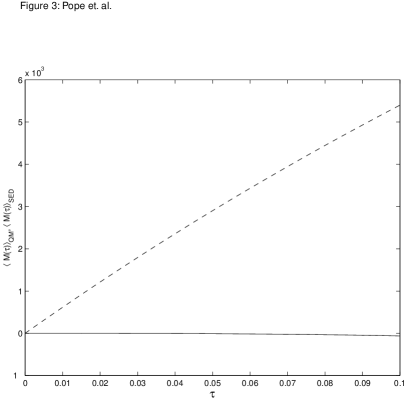
FIG. 3.: Analytic results for $\langle{\hat{M}}(\tau)\rangle_{QM}$ (solid line) and $\langle M(\tau)\rangle_{SED}$ (dotted line) versus scaled time $\tau$ for N=1, g=1, $\gamma=1$ and $\cos\Theta=\cos\Phi=1$.

FIG. 4.: Stochastic diagrams representing the lowest order nonzero terms required to determine the intracavity moment of SED $\langle M(\tau)\rangle_{SED}$ for $\beta_{i}$, where $i=1,2,3$.

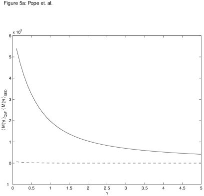
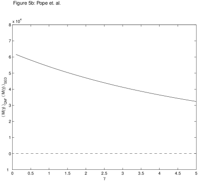
FIG. 5.: Results for $\langle{\hat{M}}(\gamma)\rangle_{QM}$ (dotted lines) and $\langle M(\gamma)\rangle_{SED}$ (solid lines) as a function of the damping constant $\gamma$ for $g=0.1,N=1$, $\cos\Theta=\cos\Phi=0$ and (a) $\tau=1$, (b) $\tau=0.1$.

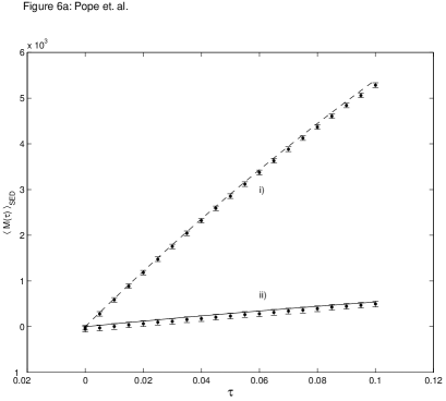
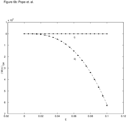
FIG. 6.: Numerical and analytic results for $\langle{\hat{M}}(\tau)\rangle_{QM}$ and $\langle M(\tau)\rangle_{SED}$ for $N=1$, $\gamma=1$ and $\cos\Theta=\cos\Phi=1$. (a) Analytic results for $\langle M(\tau)\rangle_{SED}$ for $g=0.1$ (solid line) and $g=1$ (dotted line), and numerical results for $\langle M(\tau)\rangle_{SED}$ represented by dots with associated error bars for i) $g=1$ and ii) $g=0.1$. (b) Analytic results for $\langle{\hat{M}}(\tau)\rangle_{QM}$ for $g=0.1$ (solid line) and $g=1$ (dotted line), and numerical results for $\langle{\hat{M}}(\tau)\rangle_{QM}$ represented by dots with associated error bars for i) $g=1$ and ii) $g=0.1$.

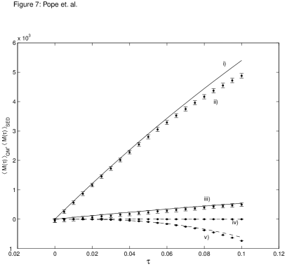
FIG. 7.: Numerical and analytic results for $\langle{\hat{M}}(\tau)\rangle_{QM}$ and $\langle M(\tau)\rangle_{SED}$ for $N=10$, $\gamma=1$ and $\cos\Theta=\cos\Phi=1$. Analytic results for $\langle M(\tau)\rangle_{SED}$ are indicated by solid lines for i) $g=1$ and iii) $g=0.1$. Numerical results for $\langle M(\tau)\rangle_{SED}$ are indicated by dots and with associated error bars for ii) $g=1$ and iii) $g=0.1$. Analytic results for $\langle{\hat{M}}(\tau)\rangle_{QM}$ are indicated by dotted lines for v) $g=1$ and iv) $g=0.1$. Numerical results for $\langle{\hat{M}}(\tau)\rangle_{QM}$ are indicated by dots with associated error bars for v) $g=1$ and iv) $g=0.1$.

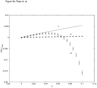
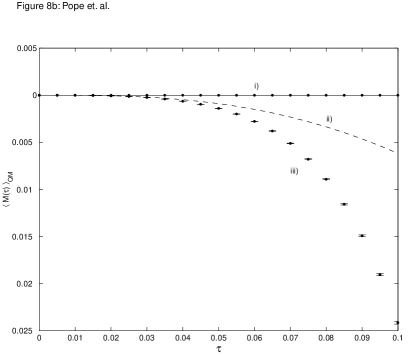
FIG. 8.: Numerical and analytic results for $\langle{\hat{M}}(\tau)\rangle_{QM}$ and $\langle M(\tau)\rangle_{SED}$ for $N=100$, $\gamma=1$ and $\cos\Theta=1=\cos\Phi=1$. (a) Numerical results for $\langle M(\tau)\rangle_{SED}$ represented by dots with associated errorbars for ii) $g=0.1$ and iii) $g=1$, and analytic results for $\langle M(\tau)\rangle_{SED}$ for $g=0.1$ (dotted line) and $g=1$ (solid line). b) Numerical results for $\langle{\hat{M}}(\tau)\rangle_{QM}$ represented by dots with associated errorbars for i) $g=0.1$ and ii) $g=1$, and analytic results for $\langle{\hat{M}}(\tau)\rangle_{QM}$ for $g=1$ (dotted line) and $g=0.1$ (solid line).

FIG. 9.: Schematic diagram for balanced homodyne detection. Photodetectors are labeled by $D_{+\>i}$ and $D_{-\>i}$, for $i=1,2,3$, BS is a beamsplitter, ${\bar{\theta}}_{i}$ is a local oscillator phase variable, $E_{i}$ is a local oscillator amplitude and ${\hat{\Phi}}_{i}$ is an external signal field operator.

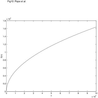
FIG. 10.: Plot of signal to noise ratio of the difference between the sample moments of quantum mechanics and SED S versus sample size n for ${\rm AgGaSe_{2}}$ for g=$8.3\times 10^{-3}$, $\tau_{f}=0.1$ and $\eta=1$.

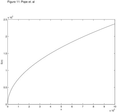
FIG. 11.: Plot of signal to noise ratio of the difference between the sample moments of quantum mechanics and SED S versus sample size n for KTP for g=$1.2\times 10^{-3}$, $\tau_{f}=0.1$ and $\eta=1$.

CRYSTAL	$d_{eff}(pmV^{-1})$	$V(m^{3})$	$\lambda_{3}\simeq\lambda_{2}/2\simeq\lambda_{1}/2(\mu m)$	$G(s^{-1})$	$\Gamma(s^{-1})$	$g(=\frac{G}{\Gamma}$)
${\rm AgGaSe_{2}}$	$33\>(at\>\lambda=2.1\mu m$) [30]	$1.0\times 10^{-9}$	$1.4$	$1.3\times 10^{5}$	$1.5\times 10^{7}$	$8.3\times 10^{-3}$
KTP	$7.2\>(at\>\lambda=2.3\mu m$) [30]	$1.6\times 10^{-9}$	$1.6$	$1.8\times 10^{4}$	$1.5\times 10^{7}$	$1.2\times 10^{-3}$

TABLE I.: Table of realistic values for the parameters $d_{eff}$, volume V, pump, signal and idler wavelengths $\lambda_{3},\lambda_{2}$ and $\lambda_{1}$, nonlinear coupling constant G, damping constant $\Gamma$ and nonlinear coupling constant to damping ratio $g$ for the nonlinear crystals ${\rm AgGaSe_{2}}$ and KTP.

CRYSTAL	$\langle{\hat{M}^{(E)}}(\tau_{f})\rangle$	$\langle M^{(E)}(\tau_{f})\rangle_{SED}$
${\rm AgGaSe_{2}}$	-$2.9\times 10^{8}$	$1.3\times 10^{9}$
KTP	$-8.8\times 10^{5}$	$1.8\times 10^{8}$

TABLE II.: Table of the external moments of quantum mechanics and SED for ${\rm AgGaSe_{2}}$ and KTP.