Temporal Ordering in Quantum Mechanics

Abstract

We examine the measurability of the temporal ordering of two events, as well as event coincidences. In classical mechanics, a measurement of the order-of-arrival of two particles is shown to be equivalent to a measurement involving only one particle (in higher dimensions). In quantum mechanics, we find that diffraction effects introduce a minimum inaccuracy to which the temporal order-of-arrival can be determined unambiguously. The minimum inaccuracy of the measurement is given by $\delta t=\hbar/{\bar{E}}$ where ${\bar{E}}$ is the total kinetic energy of the two particles. Similar restrictions apply to the case of coincidence measurements. We show that these limitations are much weaker than limitations on measuring the time-of-arrival of a particle to a fixed location.

I Introduction

In quantum mechanics, one typically measures operators at fixed times $t$. For example, one can measure the position of a particle at any given time, and obtain a precise result. One could also consider the ”dual” situation in which one tries to measure at what time a particle arrives to a fixed location $x_{a}$. This problem of time-of-arrival allcock has been extensively discussed in the literature muga .

Although the time $t$ is a well defined parameter in the Schrödinger equation, Pauli has shown that it cannot correspond to an operator for systems which have an energy bounded from below pauli . Likewise, for general Hamiltonians, there is no operator which corresponds to the time of an event such as the time-of-arrival of a particle to a fixed location aharonov . In addition, if one wishes to operationally measure the time-of-arrival by coupling the system to a clock, then one finds that one cannot measure the time-of-arrival to an accuracy better than $\hbar/{\bar{E}_{k}}$ where ${\bar{E}_{k}}$ is the kinetic energy of the particleallcock ; aharonov ; tmeas . The limitation is based on calculations from a wide variety of different measurement models, as well as general considerations, however, there is no known proof of this result.

There have been attempts to circumvent these difficulties rovelli circ muga , usually involving a modified time-of-arrival operator or POVM measurements. Such operators can be measured “impulsively” by interacting with the system at a certain (arbitrary) instant of time. In this manner, one can attempt to measure the time-of-arrival even though the particle has not arrived (and in fact, may never arrive, regardless of what the result of the time-of-arrival measurement yields)tmeas . These procedures, are hence conceptually and operationally very different from the case of continuous measurements discussed here.

One can also ask, given two events $A$ and $B$, whether one can measure which event occurred first. Surprisingly, there does not appear to be any discussion of this in the literature, even though we believe it is a much more primitive and fundamental concept. In this paper, we are interested in whether the well defined classical concepts of temporal ordering have a quantum analogue. In other words, given two quantum mechanical systems, can we measure which system attains a particular state first. Can we decide whether an event occurs in the past or future of another event.

Classically, one can couple the system to a device which is triggered when an event occurs, and records which event happened first. One can consider a similar measurement scheme in quantum mechanics which classically would correspond to a measurement of order of events. One can then ask whether such a quantum measurement scheme is possible.

The fact that there is a limitation to measurements of the time of an event leads one to suspect that the ordering of events may not be an unambiguous concept in quantum mechanics. However, for a single quantum event $A$, although one cannot determine the time an event occurred to arbitrary accuracy, it can be argued that one can often measure whether $A$ occurred before or after a fixed time $t_{B}$ to any desired precision.

Consider a quantum system initially prepared in a state $\psi(0)$ and an event $A$ which corresponds to some projection operator $\Pi_{A}$ acting on this state. For example, we could initially prepare an atom in an excited state, and $\Pi_{A}$ could represent a projection onto all states where the atom is in its ground state i.e. the atom has decayed. $\psi(0)$ could also represent a particle localized in the region $x<0$ and $\Pi_{A}$ could be a projection onto the positive x-axis. In this case, the event $A$ corresponds to the particle arriving to $x=0$.

If the state evolves irreversibly to a state for which $\Pi_{A}\psi(t)=1$, then we can easily measure whether the event $A$ has occurred at any time $t$. We could therefore measure whether a free particle arrives to a given location before or after a classical time $t_{B}$. Of course, for many systems, the system will not irreversibly evolve to the required state. For example, a particle influenced by a potential may cross over the origin many times. However, for an event such as atomic decay, the probability of the atom being re-excited is relatively small, and one can argue that the event is effectively irreversible.

For the case of a free particle which has been measured to be traveling towards the origin from $x<0$ one can argue that if at a later time we measure the projection operator onto the positive axis and find it there, then the particle must have arrived to the origin at some earlier time. This is in some sense a definition, because we know of no way to measure the particle being at the origin without altering its evolution (or being extremely lucky and happening to measure the particle’s location when it is at the origin).

While measuring whether an event happened before or after a fixed time $t_{B}$ may be possible, we will find that for two quantum events, one cannot in general measure whether the time $t_{A}$ of event $A$, occurred before or after the time $t_{B}$ of event $B$.

In Section II, confining ourselves to a particular example of order of events, we will consider the question of order of arrival in quantum mechanics. Given two particles, can we determine which particle arrived first to the location $x_{a}$. Using a model detector, we find that there is always an inherent inaccuracy in this type of measurement given by $\hbar/{\bar{E}}$ where ${\bar{E}}$ is the typical total energy of the two particles. This seems to suggest that the notion of past and future is not a well defined observable in quantum mechanics.

We will see that this inaccuracy limitation on the measurement of order-of-arrival is weaker than the inaccuracy on measurements of time-of-arrival. If one attempted to measure the order-of-arrival by measuring the time-of-arrival of both particles, then the limitation on the measurement accuracy is much greater, being $\hbar/min\{E_{x},E_{y}\}$ where $E_{x}$ and $E_{y}$ are the typical energies of each individual particle.

In the present article we will consider only continuous measurements in which the detector is left “open” for a long duration. One can also formally define an order-of-arrival operator like

$${\bf O}=sgn({\bf T_{A}}_{x}-{\bf T_{A}}_{y})$$ (1)

where $T_{x}$ and $T_{y}$ are the time-of-arrival operators

$${\bf T_{A}}=\frac{mx_{a}}{{\bf p}}-m\frac{1}{\sqrt{{\bf p}}}{\bf x}\frac{1}{\sqrt{{\bf p}}}\,\,\,\,\,.$$ (2)

As already noted, if one measures such an operator one is measuring which event occurred first, even though neither event has in fact occurred (and may not occur). The measurement of an operator, and the continuous, ”operational” methods discussed here, are therefore rather different. Furthermore, the time-of-arrival operator cannot be self-adjoint aharonov , and therefore has complex eigenvalues and eigenstates reedsimon . However, it can be modifiedrovelli . We believe that modifying the operator causes several technical as well as fundamental difficulties. For example, it has been shown oppenheim , that the eigenstates of modified time-of-arrival operators such as those in rovelli no longer describe events of arrival at a definite time. We anticipate similar difficulties for the case of the order-of-arrival operator.

In Section III we discuss measurements of coincidence. I.e., can we determine whether both particles arrived at the same time. Such measurements allow us to change the accuracy of the device before each experiment. We find that the measurement fails when the accuracy is made better than $\hbar/{\bar{E}}$.

In Section IV we discuss the relationship between ordering of events and the resolving power of “Heisenberg’s microscope“heisenberg , and argue that in general, one cannot prepare a two particle state which is always coincident to within a time of $\hbar/{\bar{E}}$. In the following we use units such that $\hbar=1$.

II Which first?

Consider two free particles (which we will label as x and y) initially localized to the right of the origin, and traveling to the left. We then ask whether one can measure which particle arrives to the origin first. The Hamiltonian for the system and measuring apparatus is given by

$${\bf H}=\frac{{\bf P_{x}}^{2}}{2m_{1}}+\frac{{\bf P_{y}}^{2}}{2m_{2}}+{\bf H}_{i}$$ (3)

where ${\bf H}_{i}$ is some interaction Hamiltonian which is used to perform the measurement. One possible choice for an interaction Hamiltonian is

$${\bf H}_{i}=\alpha\delta({\bf x})\theta(-{\bf y})$$ (4)

with $\alpha$ going to infinity.

If the y-particle arrives before the x-particle, then the x-particle will be reflected back. If the y-particle arrives after the x-particle, then neither particle sees the potential, and both particles will continue traveling past the origin. One can therefore wait a sufficiently long period of time, and measure where the two particles are. If both the x and y particles are found past the origin, then we know that the x-particle arrived first. If the y-particle is found past the origin while the x-particle has been reflected back into the positive x-axis then we know that the y-particle arrived first.

Classically, this method would appear to unambiguously measure which of the two particle arrived first. However, in quantum mechanics, this method fails. From (3) we can see that the problem of measuring which particle arrives first is equivalent to deciding where a single particle traveling in a plane arrives. Two particles localized to the right of the origin is equivalent to a single particle localized in the first quadrant (see Figure 1). The question of which particle arrives first, becomes equivalent to the question of whether the particle crosses the positive x-axis or the positive y-axis.

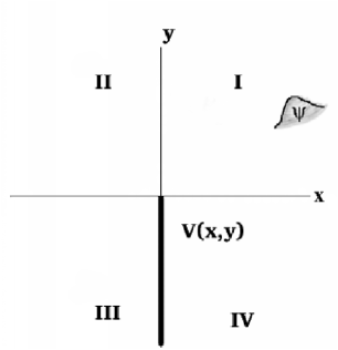
Figure 1: The measurement of order-of-arrival for two particles in one dimension, is equivalent to scattering of a straight edge of one particle in two-dimensions.

The equivalence between the two-particle system and the single particle system in higher dimensions can be seen by performing the canonical transformation

$${\bf P_{x}} \longrightarrow \sqrt{m_{1}\over M}{\bf P_{x}},\ \ \ \ {\bf P_{y}}\longrightarrow\sqrt{m_{2}\over M}{\bf P_{y}}$$

$${\bf x} \longrightarrow \sqrt{M\over m_{1}}{\bf x},\ \ \ \ \ \ {\bf y}\longrightarrow\sqrt{M\over m_{2}}{\bf y}$$ (5)

and rescaling $\alpha\to\sqrt{M/m_{1}}\alpha$. Our Hamiltonian now looks like that of a single particle of mass $M$ scattering off a thin edge in two dimensions. Classically, the event $x$ arriving first, corresponds to the case that the particle does not scatter off the edge and travels to quadrant III. The event of $y$ arriving first corresponds to scattering off the edge to quadrant IV.

However, quantum mechanically, we find that sometimes the particle is found in the two classically forbidden regions, I and II. If the particle is found in either of these two regions, then we cannot determine which particle arrived first.

The solution for a plane wave which makes an angle $\theta_{o}$ with the x-axis is well knownmorseandf . If the boundary condition is such that $\psi(r,\theta)=0$ on the negative y-axis, then the solution is

$$\psi(r,\theta)=\frac{1}{\sqrt{i\pi}}\left\{e^{-ikr\cos(\theta-\theta_{o})}\Phi[\sqrt{2kr}\cos(\frac{\theta-\theta_{o}}{2})]-e^{ikr\cos(\theta+\theta_{o})}\Phi[-\sqrt{2kr}\sin(\frac{\theta+\theta_{o}}{2})]\right\}$$ (6)

where $\Phi(z)$ is the error function.

Asymptotically, this solution looks like

$$\psi\simeq\left\{\begin{array}[]{ll}e^{-ikr\cos(\theta-\theta_{o})}+f(\theta)\frac{e^{ikr}}{\sqrt{r}}&-\theta_{o}<\theta<\pi+\theta\\ e^{-ikr\cos(\theta-\theta_{o})}-e^{ikr\cos(\theta+\theta_{o})}+f(\theta)\frac{e^{ikr}}{\sqrt{r}}&-\theta_{o}>\theta>-\pi/2\\ f(\theta)\frac{e^{ikr}}{\sqrt{r}}&\pi-\theta_{o}<\theta<3\pi/2\end{array}\right.$$ (7)

where

$$f(\theta)=-\sqrt{\frac{i}{8\pi k}}\left[\frac{1}{\sin(\frac{\theta+\theta_{o}}{2})}+\frac{1}{\cos(\frac{\theta-\theta_{o}}{2})}\right]\,\,.$$ (8)

The above approximation is not valid when $\cos(\frac{\theta-\theta_{o}}{2})$ or $\sin(\frac{\theta+\theta_{o}}{2})$ is close to zero.

Since we demanded that the particle was initially localized in the first quadrant, the initial wave cannot be an exact plane wave, but we can imagine that it is a plane wave to a good approximation.

We see from the solution above that the particle can be found in the classically forbidden regions of quadrant I and II. For these cases, we cannot determine which particle arrived first. This is due to interference which occurs when the particle is close to the origin (the sharp edge of the potential). The amplitude for being scattered off the region around the edge in the direction $\theta$ is given by $|f(r,\theta)|^{2}$.

It might be argued that since these particles scattered, they must have scattered off the potential, and therefore they represent experiments in which the y-particle arrived first. However, this would clearly over count the cases where the y-particle arrived first. We could have just as easily have placed our potential on the negative x-axis, in which case, we would over-count the cases where the x-particle arrived first.

In the ”interference region” we cannot have confidence that our measurement worked at all. We should therefore define a ”failure cross section” given by

$$\sigma_{f} = \int_{0}^{2\pi}|f(\theta)|^{2}$$ (9)

$$= \frac{1}{k\cos(\frac{\theta_{o}}{2})}$$

From (9) we can see that cross section for scattering off the edge is the size of the particle’s wavelength multiplied by some angular dependence. Therefore, if the particle arrives within a distance of the origin given by

$$\delta x>2/k\,\,\,\,\,\,$$ (10)

the measurement will fail. We have dropped the angular dependence from (9) – the angular dependence is not of physical importance for measuring which particle came first, as it depends on the details of the potential (boundary conditions) being used. The particular potential we have chosen is not symmetrical in x and y.

From this we can conclude that if the particle arrives to within one wavelength of the origin, then there is a high probability that the measurement will fail.

If we want to relate this two-dimensional scattering problem back to two particles traveling in one dimension, we need to use the relation

$$\delta t\simeq\frac{m\delta x}{k}$$ (11)

In other words, our measurement procedure relies on making an inference between time measurements and spatial coordinates. The last two equations then give us

$$\delta t>\frac{1}{E}\,\,\,\,\,\,.$$ (12)

One will not be able to determine which particle arrived first, if they arrive within a time $1/E$ of each other, where $E$ is the total kinetic energy of both particles. Note that Equation (12) is valid for a plane wave with definite momentum $k$. For wave functions for which $dk<<k$, one can replace $E$ by the expectation value $\langle E\rangle$. However, for wave functions which have a large spread in momentum, or which have a number of distinct peaks in $k$, then to ensure that the measurement almost always works, one must measure the order of arrival with an accuracy given by

$$\delta t>\frac{1}{{\bar{E}}}$$ (13)

where ${\bar{E}}$ is the minimum typical total energy . Hence we conclude that if the particles are coincident to within $1/{\bar{E}}$, then the measurement fails.

It is rather interesting that this measurement limitation is less strict than the one obtained if we were to measure the time-of-arrival of each particle individually. This can be seen from the mapping of Eq. 5 since the total energy ${\bar{E}}=E_{x}+E_{y}$ where $E_{x}$ and $E_{y}$ are the energies of each individual particle. The limitation on measurements of the time-of-arrival of each particle is given by $1/E_{x}$ and $1/E_{y}$ aharonov . Therefore, if we use time of arrival measurements to determine the order of arrival, the minimal inaccuracy will have to be $1/min\{E_{x},E_{y}\}$ which can be considerably worse than $1/(E_{x}+E_{y})$ using the method outlined above.

The extreme limit, where one of the particles has a very high energy is then rather interesting. We have argued in the previous section that for the case of a single event, we can measure with arbitrary accuracy if the event occurred before or after a certain given time $t_{0}$. Indeed, let us consider the above setup in the special limit that $E_{y}\gg E_{x}$ with $E_{y}\to\infty$. The diffraction pattern in this case is completely controlled by the $y$ particle and $\delta t>{1\over\bar{E}}\sim{1\over E_{y}}\to 0$. Furthermore for the case $dy\ll dE_{y}\ll E_{y}$, the location $y$ of the energetic particle can serve as a good “clock”bennicasher and has a well defined time-of-arrival to $y=0$. Hence the initial state of the $y$ particle defines (up to $1/E_{y}\to 0$) the time-of-arrival of the y-particle, $t_{0}=t_{A}(y=0)$. The final states of the “clock” hence determines whether the $x$ particle arrived before or after $t=t_{0}$. If $y_{final}>0$ we conclude that $t_{A}(x=0)<t_{0}$ and if $y_{final}<0$ that $t_{A}(x=0)>t_{0}$.

On can create a full clock, by considering many heavy ”y” particles, and determining whether the ”x” particle came before or after each one of them. Increasing the number of ”y” particles and having them arrive at regularly spaced intervals would then constitute a measurement of time-of-arrival. We would then expect to recover the limitation of reference aharonov as the density of ”y” is increased.

III Coincidence

In the previous model for measuring which particle arrived first, we found that if the two particles arrived to within $1/{\bar{E}}$ of each other, the measurement did not succeed. The width $1/{\bar{E}}$ was an inherent inaccuracy which could not be overcome. However, in our simple model, we were not able to adjust the accuracy of the measurement.

It is therefore instructive to consider a measurement of “coincidence” alone for which one can quite naturally adjust the accuracy of the experiment. Given two particles traveling towards the origin, we ask whether they arrive within a time $\delta t_{c}$ of each other. If the particles do not arrive coincidently, then we do not concern ourselves with which arrived first. The parameter $\delta t_{c}$ can be adjusted, depending on how accurate we want our coincident “sieve” to be. We will once again find that one cannot decrease $\delta t_{c}$ below $1/{\bar{E}}$ and still have the measurement succeed.

A simple model for a coincidence measuring device can be constructed in a manner similar to (4). Mapping the problem of two particles to a single particle in two dimensions, we could consider an infinite potential strip of length $2a$ and infinitesimal thickness, placed at an angle of $\pi/4$ to the x and y axis in the first quadrant (see Figure 2). Particles which miss the strip, and travel into the third quadrant are not coincident, while particles which bounce back off the strip into the first quadrant are measured to be coincident. I.e. if the x-particle is located within a distance $a$ of the origin when the y-particle arrives (or visa versa), then we call the state coincident.

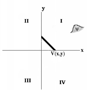
Figure 2: Potential for measuring whether two particles are coincident.

Classically, one expects there to be a sharp shadow behind the strip. Quantum mechanically, we once again find an interference region around the strip which scatters particles into the classically forbidden regions of quadrant two and four. The shadow is not sharp, and we are not always certain whether the particles were coincident.

A solution to plane waves scattering off a narrow strip is well known and can be found in many quantum mechanical texts (see for example morseandf where the scattered wave is written as a sum of products of Hermite polynomials and Mathieu functions). However, for our purposes, we will find it convenient to consider a simpler model for measuring coincidence, namely, an infinite circular potential of radius $a$, centered at the origin.

$$H_{i}=\alpha V(r/a)$$ (14)

where $V(x)$ is the unit disk, and we take the limit $\alpha\rightarrow\infty$.

It is well known that if $a<1/k$, then there will not be a well-defined shadow behind the disk. To see this, consider a plane wave coming in from negative x-infinity. It can be expanded in terms of the Bessel function $J_{m}(kr)$ and then written asymptotically ($r\gg 1$) as a sum of incoming and outgoing circular waves.

$$e^{ikx} = \sum_{m=0}^{\infty}\epsilon_{m}i^{m}J_{m}(kr)\cos{m\theta}$$ (15)

$$\simeq \sqrt{\frac{1}{2\pi ikr}}\left[e^{ikr}\sum_{m=0}^{\infty}\epsilon_{m}\cos{m\theta}+ie^{-ikr}\sum_{m=0}^{\infty}\epsilon_{m}\cos{m(\theta-\pi)}\right]\,\,\,.$$

where $\epsilon_{m}$ is the Neumann factor which is equal to 1 for $m=0$ and equal to 2 otherwise.

Since it can be shown that

$$\sum_{m=0}^{M}\epsilon_{m}\cos{m\theta}=\frac{\sin{(M+\frac{1}{2})\theta}}{\sin{\frac{1}{2}\theta}}$$ (16)

The two infinite sums approach $2\pi\delta(\theta)$ and $2\pi\delta(\theta-\pi)$ respectively, and so the incoming wave comes in from the left, and the outgoing wave goes out to the right. The presence of the potential modifies the wave function and in addition to the plane wave, produces a scattered wave

$$\psi=e^{ikx}+\frac{e^{ikr}}{\sqrt{r}}f(r\theta)$$ (17)

where

$$\frac{e^{ikr}}{\sqrt{r}}f(r,\theta)=-i\sum_{m=0}^{\infty}\epsilon_{m}e^{\frac{1}{2}m\pi i-i\delta_{m}}\sin{\delta_{m}}H_{m}(kr)\cos{m\theta}\,\,\,\,\,,$$ (18)

$H_{m}(kr)$ are Hermite polynomials and

$$\tan{\delta_{m}}=\frac{-J_{m}(ka)}{N_{m}(ka)}$$ (19)

($N_{m}(ka)$ are Bessel functions of the second kind). For large values of $r$, the wave function can be written in a manner similar to (15), except that the outgoing wave is modified by the phase shifts $\delta_{m}$.

$$\psi\simeq\frac{1}{\sqrt{2\pi ik}}i\sum_{m=0}^{\infty}\epsilon_{m}\cos{m(\theta-\pi)}\frac{e^{-ikr}}{\sqrt{r}}+\frac{e^{ikr}}{\sqrt{r}}f(r,\theta)\,\,\,,$$ (20)

where

$$f(r,\theta)\simeq\frac{1}{\sqrt{2\pi ik}}\sum_{m=0}^{\infty}\epsilon_{m}e^{-2i\delta_{m}(ka)}\cos{m\theta}$$ (21)

In the limit that $ka\gg m$ the phase shifts can be written as

$$\delta_{m}\simeq ka-\frac{\pi}{2}(m+\frac{1}{2})\,\,\,\,.$$ (22)

In the limit of extremely large $a$ (but $r\gg a$), the outgoing waves then behave as

$$f(r,\theta)\simeq\lim_{M\rightarrow\infty}-i\frac{1}{\sqrt{2\pi ik}}e^{-2ika}\frac{\sin{(M+\frac{1}{2})(\theta-\pi)}}{\sin{\frac{1}{2}(\theta-\pi)}}$$ (23)

where once again we see that the angular distribution goes as the delta function $\delta(\theta-\pi)$. The disk scatters the plane wave directly back, and a sharp shadow is produced. We see therefore, that in the limit of $ka\gg 1$, our measurement of coincidence works.

The differential cross section can in general be written as

$$\sigma = |f(\theta)|^{2}$$ (24)

$$= |\sum_{m=0}^{\infty}\epsilon_{m}e^{-2i\delta_{m}(ka)}\cos{m\theta}|^{2}$$

For $ka\gg 1$ (but still finite), (24) can be computed using our expression for the phase shifts from (22), and is given by

$$\sigma(\theta)\simeq\frac{a}{2}\sin{\frac{\theta}{2}}+\frac{1}{2\pi k}\cot^{2}{\frac{\theta}{2}}\sin^{2}{ka\theta}$$ (25)

The first term represents the part of the plane wave which is scattered back, while the second term is a forward scattered wave which actually interferes with the plane-wave. The reason it appears in our expression for the scattering cross section is because we have written our wave function as the sum of a plane-wave and a scattered wave, and so part of the scattered wave must interfere with the plane-wave to produce the shadow behind the disk.

For $ka\ll m$, the phase shifts look like

$$\delta_{m}(ka)\simeq\frac{\pi m}{(m!)^{2}}\left(\frac{ka}{2}\right)^{2m}\,\,\,\,\,\,\,\,\,\,\,m\neq 0$$ (26)

and

$$\tan{\delta_{0}(ka)}\simeq\frac{-\pi}{2\ln{ka}}$$ (27)

As a result, for $ka\ll 1$, $\delta_{0}$ is much greater than all the other $\delta_{m}$ and the outgoing solution is almost a pure isotropic s-wave.

For $ka\ll 1$ the only contribution to (24) comes from $\delta_{0}$ and the differential cross section becomes

$$\sigma(\theta)\simeq\frac{\pi}{2k\ln^{2}{ka}}$$ (28)

and is isotropic. In other words, no shadow is formed at all, and particles are scattered into classically forbidden regions. We see therefore, that as long as the s-wave is dominant, our measurement fails. The s-wave will cease being dominant when $\delta_{0}$ is of the same order as $\delta_{1}$. As can be seen from (22), $\delta_{1}/\delta_{0}$ approaches a limiting value of $1$ when a sharp shadow is produced. It is only when $\delta_{1}/\delta_{0}\simeq 1$ that the cross-section no longer depends on $k$. This is what we require then, for the probability of our measurement to succeed independently of the energy of the incoming particles. From a plot of $\delta_{1}/\delta_{0}$ we see that this only occurs when $ka\gg 1$ (Figure 5). Our condition for an accurate measurement is therefore that $a\gg 1/k$. Since $\delta t_{c}\simeq am/k$ we find

$$\delta t_{c}\gg 1/E$$ (29)

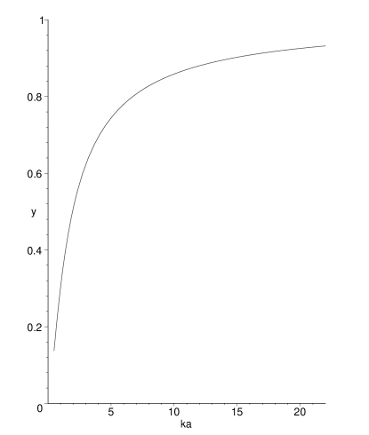
Figure 3: $\delta_{1}(ka)/\delta_{0}(ka)$ vs. $ka$

IV Coincident States

We have seen that we can only measure coincidence to an accuracy of $\delta t_{c}=1/{\bar{E}}$. We shall now show that one cannot prepare a two particle system in a state $\psi_{c}$ which always arrives coincidentally within a time less than $\delta t_{c}$. In other words, one cannot prepare a system in a state which arrives coincidentally to greater accuracy than that set by the limitation on coincidence measurements.

Preparing a state $\psi_{c}$ corresponds to preparing a single particle in two dimensions which always arrives inside a region $\delta r=p\delta t_{c}/m$ of the origin. In other words, suppose we were to set up a detector of size $\delta r$ at the origin. If a state $\psi_{c}$ exists, then it would always trigger the detector at some later time.

Our definition of coincidence requires that the state $\psi_{c}$ not be a state where one particle arrives at a time $t>\delta t_{c}$ before the other particle. In other words, if instead, we were to perform a measurement on $\psi_{c}$ to determine whether particle x arrived at least $\delta t_{c}$ before particle y, then we must get a negative result for this measurement.

This latter measurement would correspond to the two-dimensional experiment of placing a series of detectors on the positive y-axis, and measuring whether any of them are triggered by $\psi_{c}$. If $\psi_{c}$ is truly a coincident state, then none of the detectors which are placed at a distance greater than $y=\delta r$ can be triggered. One could even consider a single detector, placed for example, at $(0,{\delta r})$, and one would require that $\psi_{c}$ not trigger this detector.

Now consider the following experiment. We have a particle detector which is either placed at the origin, or at $(0,{\delta r})$ (we are not told which). Then after a sufficient length of time, we observe whether it has been triggered. If we can prepare a coincident state $\psi_{c}$, then it will always trigger the detector when the detector is at the origin, but never trigger the detector when the detector is at $(0,{\delta r})$. This will allow us to determine whether the detector was placed at the origin, or at $(0,{\delta r})$. For example, if we use the detectors described in Section III (namely, just a scattering potential), then some of the time, the particle will be scattered, and some of the time it won’t be, and if it is scattered, we can conclude that the potential was centered around the origin rather than around $(0,{\delta r})$.

However, as we know from Heisenberg’s gedanken microscope experiment, a particle cannot be used to resolve anything greater than it’s wavelength. In other words $\psi_{c}$ cannot be used to determine whether the detector is at the origin, or at $(0,{\delta r})$ if ${\delta r}<2\pi/k$. As a result, $\psi_{c}$ can only be coincident to a region around the origin of radius less than ${\delta r}$ or, coincident within a time $\delta t_{c}\sim 1/E$.

V Conclusion

The notion that events proceed in a well defined sequence is unquestionable in classical mechanics. Events occur one after the other, and our knowledge concerning the events at one time allows us to predict what will occur at another time. One can unambiguously determine whether events lie in the past or future of other events. Given two events, $A$ and $B$, one can compute which event occurred first. It may be, that event $A$ causes event $B$, in which case, event $A$ must have preceded event $B$.

However, in quantum mechanics the situation is different. We have argued that we cannot measure the order of arrival for two free particles if they arrive within a time of $1/{\bar{E}}$ of each other, where ${\bar{E}}$ is their typical total kinetic energy. If we try to measure whether they arrive within a time $\delta t_{c}$ of each other, then our measurement fails unless we have at least $\delta t_{c}>1/{\bar{E}}$. Furthermore, we cannot construct a two particle state where both particles arrive to a certain point within a time of $1/{\bar{E}}$ of each other.

Interestingly, this inaccuracy limitation is weaker than what would be obtained if one tried to measure the time-of-arrival of each particle separately.

It may be interesting to consider the situation where we have an event B which must be preceded by an event A. For example, B could be caused by A, or the dynamics could be such that B can only occur when the system is in the state A. One can then attempt to force B to occur as close to the occurrence of event A as possible. A related problem has been studied in connection to the maximum speed of dynamical systems such as quantum computers dynamical and it was found that one cannot force the system to evolve at a rate greater than $1/\bar{E}$ (where $\bar{E}$ is the average energy), rather than $1/dE$ (where $dE$ is the uncertainty in the energy). However since this result concerns only the free evolution of the system between states, it is not clear a priori that it is indeed related to the $1/\bar{E}$ restriction found in the present case where the measurement interaction disturbs the system.

Acknowledgments: J.O would like to thank Yakir Aharonov and and Mark Halpern for valuable discussion. W.G.U. acknowledges the CIAR and NSERC for support during the completion of this work. J.O. also acknowledges NSERC for their support. B.R. acknowledges the support from grant 471/98 of the Israel Science Foundation, established by the Israel Academy of Sciences and Humanities.

References

- (1) W. Pauli, Die allgemeinen Prinzipien der Wellenmechanik, in Handbook of physics, eds. H. Geiger and K. Schell, Vol. 24 Part 1, (Berlin, Springer Verlag), 1958.
- (2) G.R. Allcock, Ann Phys 53 (1969), 253
- (3) For a review of developments on the arrival time problem see for example J. G. Muga and C. R. Leavens, Phys. Rep. 338, (2000), 353. or J.G. Muga, R. Sala, J.P. Palao (quant-ph/9801043), Superlattice Microst 23: (3-4) 833-842 1998.
- (4) Y. Aharonov, J. Oppenheim, S. Popescu, B. Reznik, W.G. Unruh, (quant-ph/9709031), Phys. Rev. A 57, 4130 (1998)
- (5) N. Grot, C. Rovelli, R. S. Tate, Phys. Rev. A54, 4676 (1996), quant-ph/9603021.
- (6) The problem of time-of-arrival has also been discussed in the context of POVM’s (e.g. P. Busch, M. Grabowski, P.J. Lahti, Phys. Lett. A 191 (1994) 357). Distributional approaches e.g. J. Kijowski, Rep. Math. Phys. 6, 361 (1974); A. Baute; I. Egusquiza, J. Muga PRA 64, 012501 (2001); Or within Bohmian mechanics - C.R. Leavens, Phys. Rev. A 58 (1998) 840; M. Daumer, in: J.T. Cushing, A. Fine, S. Goldstein (Eds.), Bohmian Mechanics and Quantum Theory: An Appraisal, Kluwer, Dordrecht, 1996; The interested reader is referred to reference [3] for a review of the various approaches.
- (7) J. Oppenheim, B. Reznik, W.G. Unruh, quant-ph/9805064, Found. Phys. .This work also contains arguments on why time-of-arrival distributions can be problematic, even in the classical case.
- (8) M. Reed and B. Simon, Methods of Modern Mathematical Physics II: Fourier Analysis, Self-Adjointness, New York, Academic Press, 1975.
- (9) J. Oppenheim, B. Reznik, W.G. Unruh,Phys. Rev. A, 59 1804 (1999), quant-ph/9801034; see also Muga, Leavens and Palao, Phys. Rev. A 58 (1998) 4336.
- (10) For a discussion of this, see A. Casher, B. Reznik ”Back-Reaction of Clocks and Limitations on Observability in Closed Systems”, quant-ph/9909010, to appear in Phys. Rev. A
- (11) W. Heisenberg, Zeitschrift für Physik, 43, 172-198 (1927), reprinted in Quantum Theory and Measurement, J. A. Wheeler and W.H. Zurek, eds (Princeton Univ. Press, 1983)
- (12) See for example, Morse and Feshbach, Methods of Theoretical Physics, McGraw-Hill Book company, New York, 1953 or the rigorous M. Reed and B. Simon, Methods of Modern Mathematical Physics III: Scattering Theory, New York, Academic Press, 1975.
- (13) N. Margolus, L. Levitin, Physica D120 (1998) 188-195, quant-ph/9710043