Separability properties of tripartite states with $\rm U\!\otimes\!U\!\otimes\!U$-symmetry

Abstract

We study separability properties in a $5$-dimensional set of states of quantum systems composed of three subsystems of equal but arbitrary finite Hilbert space dimension. These are the states, which can be written as linear combinations of permutation operators, or, equivalently, commute with unitaries of the form $U\otimes U\otimes U$. We compute explicitly the following subsets: (1) triseparable states, which are convex combinations of triple tensor products, (2) biseparable states, which are separable for a twofold partition of the system, and (3) states with positive partial transpose with respect to such a partition.

I Introduction

One of the difficulties in the theory of entanglement is that state spaces are usually fairly high dimensional convex sets. Therefore, to explore in detail the potential of entangled states one often has to rely on lower dimensional “laboratories”. An example of this was the role played by a one-dimensional family of bipartite states [1], which has come to be known as “Werner states”. In this paper we present a similar laboratory, designed for the study of entanglement between three subsystems. The basic idea is rather similar to [1], and we believe this set shares many of the virtues with its bipartite counterpart. Firstly, the states have an explicit parametrization as linear combinations of permutation operators. This is helpful for explicit computations. Secondly, there is a “twirl” operation which brings an arbitrary tripartite state to this special subset. This proved to be very helpful for the discussion of entanglement distillation of bipartite entanglement: the first useful distillation procedures worked by starting with Werner states, applying a suitable distillation operation, and then the twirl projection to come back to the simple and well understood subset, thus allowing iteration. Geometrically this means that the subset we investigate is both a section of the state space by a hyperplane and the image of the state space under a projection. The basic technique for getting such subsets is averaging over a symmetry group of the entire state space. Such an averaging projection preserves entanglement if it is an average only over local (factorizing) unitaries (see [2] for a recent example different from ours).

The third useful property of the states we study is that they can be defined for systems of arbitrary finite Hilbert space dimension $d$, which is again important for the discussion of distillation. Surprisingly, it even turns out that in the parametrization we choose all the sets we investigate are also independent of dimension.

We now describe the entanglement (or separability) properties we will chart for these special states. Of course, we can split the system into just two subsystems and apply the usual separability/entanglement distinctions. A split $1|23$ then corresponds to the grouping of the Hilbert space ${\cal H}_{1}\otimes{\cal H}_{2}\otimes{\cal H}_{3}$ into ${\cal H}_{1}\otimes({\cal H}_{2}\otimes{\cal H}_{3})$. We call a density operator $\rho$ on this Hilbert space $1|23$-separable ($\rho\in{\cal B}_{1}$), or just biseparable if the partition is clear from the context, if we can write

$$\rho=\sum_{\alpha}\lambda_{\alpha}\ \rho^{(1)}_{\alpha}\otimes\rho^{(23)}_{\alpha},$$ (1)

with $\lambda_{\alpha}\geq 0$ and density operators $\rho^{(23)}_{\alpha}$ on ${\cal H}_{2}\otimes{\cal H}_{3}.$ Furthermore, as it is a necessary condition for biseparability (cf. Peres [3]), we are going to look at those states having a positive partial transpose with regard to such a split. Recall that the partial transpose $A\mapsto A^{T_{1}}$ of operators on ${\cal H}_{1}\otimes{\cal H}_{2}$ is defined by

$$(\sum_{\alpha}A_{\alpha}\otimes B_{\alpha})^{T_{1}}=\sum_{\alpha}A_{\alpha}^{T}\otimes B_{\alpha},$$ (2)

where $A^{T}$ on the right hand side is the ordinary transposition of matrices with respect to a fixed basis.

As a genuinely “tripartite” notion of separability, we consider states, called triseparable (or “three-way classically correlated”), which can be decomposed as

$$\rho=\sum_{\alpha}\lambda_{\alpha}\ \rho^{(1)}_{\alpha}\otimes\rho^{(2)}_{\alpha}\otimes\rho^{(3)}_{\alpha},$$ (3)

where $\lambda_{\alpha}\geq 0$, and the $\rho^{(i)}_{\alpha}$ are density operators on the respective Hilbert spaces.

The detailed computations leading to the results presented here will be published elsewhere, together with the discussion of further aspects, such as violations of Bell inequalities, and some distillability relations.

II Description of the states

We consider only the case, where ${\cal H}_{1}={\cal H}_{2}={\cal H}_{3}={\cal H}$ is $d$-dimensional ($2\leq d<\infty$). Then the set of states we are going to study, which will be denoted by ${\cal W}$, is the set of density operators, which commute with all unitaries of the form $U\otimes U\otimes U$. The subsets of ${\cal W}$ we will compute will be denoted by ${\cal B}_{1}$, for the $1|23$-biseparable states, ${\cal P}_{1}$ for the states with positive partial transpose with respect to $1|23$, and by ${\cal T}$ for the triseparable states. Of course, ${\cal T}\subset{\cal B}_{1}\subset{\cal P}_{1}\subset{\cal W}$. We will see that all these inclusions are strict, even if we take biseparability with respect to all three partitions: ${\cal T}\neq({\cal B}_{1}\cap{\cal B}_{2}\cap{\cal B}_{3})$.

It is a fundamental fact from the representation theory of classical groups [4] that these states are precisely those which can be written as a linear combination of permutation operators

$$\rho\in{\cal W}\Leftrightarrow\rho=\sum_{\pi}\mu_{\pi}V_{\pi}$$ (4)

with coefficients $\mu_{\pi}\in{\mathbb{C}}$ and the unitary permutation operators $V_{\pi}$ defined by

$$V_{\pi}\ \phi_{1}\otimes\phi_{2}\otimes\phi_{3}=\phi_{\pi^{-1}1}\otimes\phi_{\pi^{-1}2}\otimes\phi_{\pi^{-1}3}$$

implementing the permutation symmetry of the three sites. For density operators hermiticity and normalization reduce the $3!=6$ complex parameters to five real ones (an explicit choice will be made below).

As usual, the integral

$${\bf P}\rho=\int\!dU\ (U\otimes U\otimes U)\rho\,(U\otimes U\otimes U)^{*},$$ (5)

with respect to the normalized invariant measure “$dU$” of the unitary group ${\rm U}_{d}$ defines a twirl operation with the property $\rho\in{\cal W}\iff{\bf P}\rho=\rho$.

Up to here all statements generalize easily to an arbitrary number of factors, and some are even valid for an arbitrary averaging operation with respect to a compact symmetry group. However, to carry the analysis further one needs at least a precise description of the range of the coefficients $\mu_{\pi}$ in equation (4), such that the sum indeed represents a density operator. In general this is difficult, although sometimes [2] one even gets a simplex. In the case we study in this paper, the positivity of (4) is best seen by using the following basis, rather than the set of permutation operators themselves.

$$R_{+}\! = \frac{1}{6}\bigl{(}{\openone}+V_{(12)}+V_{(23)}+V_{(31)}+V_{(123)}+V_{(321)}\bigr{)}$$ (7)

$$R_{-}\! = \frac{1}{6}\bigl{(}{\openone}-V_{(12)}-V_{(23)}-V_{(31)}+V_{(123)}+V_{(321)}\bigr{)}$$ (8)

$$R_{0} = \frac{1}{3}\Bigl{(}2\cdot{\openone}-V_{(123)}-V_{(321)}\Bigr{)}$$ (9)

$$R_{1} = \frac{1}{3}\Bigl{(}2V_{(23)}-V_{(31)}-V_{(12)}\Bigr{)}$$ (10)

$$R_{2} = \frac{1}{\sqrt{3}}\ \Bigl{(}V_{(12)}-V_{(31)}\Bigr{)}$$ (11)

$$R_{3} = \frac{i}{\sqrt{3}}\ \Bigl{(}V_{(123)}-V_{(321)}\Bigr{)}\;,$$ (12)

where we have used cycle notation to represent permutations. Then $R_{+},$ $R_{-}$ and $R_{0}$ are orthogonal projections commuting with all $V_{\pi}$, and adding up to one. The $R_{i}$ for $i=1,2,3$ fulfill the Pauli commutation relations $\left[R_{i},R_{\pm}\right]_{-}={\bf 0},$ $R_{i}^{2}=R_{0}$, and $R_{1}R_{2}=iR_{3}$ and cyclic. Now every operator $\rho$ in the linear span of the permutations can be decomposed into the orthogonal parts $R_{+}\rho$, $R_{-}\rho$, and $R_{0}\rho$, and positivity of $\rho$ is equivalent to the positivity of all three operators. This leads to the following Criterion:

Criterion 1

For any operator $\rho$ on ${\cal H}\otimes{\cal H}\otimes{\cal H}$, define the six parameters $r_{k}(\rho)=\mathop{\rm tr}\nolimits(\rho R_{k})$, for $k\in\{+,-,0,1,2,3\}$. Then $r_{k}({\bf P}\rho)=r_{k}(\rho)$. Moreover, each $\rho\in{\cal W}$ is uniquely characterized by the tuple $(r_{+},r_{-},r_{0},r_{1},r_{2},r_{3})\in{\mathbb{R}}^{6}$, and such a tuple belongs to a density matrix $\rho\in{\cal W}$ if and only if

$$r_{+},r_{-},r_{0}\geq 0, r_{+}+r_{-}+r_{0}=1$$ (13)

$${\rm and} r_{1}^{2}+r_{2}^{2}+r_{3}^{2}\leq r_{0}^{2}.$$ (14)

Taking $r_{0}=1-r_{+}-r_{-}$ to be redundant, we get a simple representation of ${\cal W}$ as a convex set in $5$ dimensions.

Note that in this parametrization the set ${\cal W}$ does not depend on the dimension $d$ with one exception: for $d=2$ the anti-symmetric projection $R_{-}$ is simply zero, so for qubits we get the additional constraint $r_{-}=0.$ Although in the case of three Qubits the dimensionality of the set is the same as in [2] the two sets differ. In fact the set presented in [2] can be obtained by averaging over a group of local unitaries of order 24.

With this parametrization we can describe the 5 dimensional set ${\cal W}$ by the points lying in the $(r_{+},r_{-})$ plane together with a point $(r_{1},r_{2},r_{3})$ in the corresponding Bloch sphere of radius $r_{0}=1-r_{+}-r_{-}$. We note that a state $\rho\in{\cal W}$ is invariant under cyclic permutations iff $r_{1}=r_{2}=0$, invariant under the interchange $2\leftrightarrow 3$ iff $r_{2}=r_{3}=0$, and invariant under all permutations iff $r_{1}=r_{2}=r_{3}=0$. The latter set will be denoted by ${\cal W}^{0}$.

III Results

The basic results are summarized in Figure 1. On the one hand, each point in this triangle corresponds to a density matrix $\rho\in{\cal W}$ with $r_{1}=r_{2}=r_{3}=0$, i.e., a permutation invariant state. On the other hand, each such point stands for the collection of states with the specified $(r_{+},r_{-})$, and arbitrary $(r_{1},r_{2},r_{3})$, all of which are projected to the state with vanishing $(r_{1},r_{2},r_{3})$ upon permutation averaging. For qubits, one always has $r_{-}=0$, so only the abscissa EB remains. Otherwise all statements are valid in any dimension $d$.

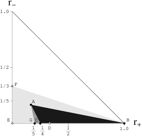
FIG. 1.: The permutation invariant subset ${\cal W}^{0}\subset{\cal W}$. Black: ${\cal T}\cap{\cal W}^{0}$; black or dark grey: ${\cal B}_{1}\cap{\cal W}^{0}$; light grey: projection of ${\cal B}_{1}$ onto ${\cal W}^{0}$ by permutation averaging. Marked points: see text.

A Triseparable States

The black triangle ABC in Figure 1 is the set of triseparable states. Its vertices are obtained by taking suitable pure product states $|\Psi\rangle\!\langle\Psi|$ with $\Psi=\phi_{1}\otimes\phi_{2}\otimes\phi_{3}$, ($\|\phi_{i}\|=1$), and applying the averaging projection ${\bf P}$. Then one gets the points A,B,C, if for $i\neq j$

$$A \mathpunct{:} \quad\langle\phi_{i}|\phi_{j}\rangle=0$$ (15)

$$B \mathpunct{:} \quad\langle\phi_{i}|\phi_{j}\rangle=1$$ (16)

$$C \mathpunct{:} \quad\langle\phi_{i}|\phi_{j}\rangle=\cos(2\pi/3)\;.$$ (17)

Note that the “Mercedes Star” configuration for $C$ requires only two dimensions, whereas $A$ requires $d\geq 3$. The technique for getting all of ${\cal T}$ is similar: an arbitrary pure product state is projected into ${\cal W}$, and ${\cal T}$ is computed as the convex hull of these points. This is more difficult than it sounds, and the details will be presented elsewhere. The result can be summarized as follows.

Criterion 2

A state $\rho\in{\cal W}$ is triseparable if and only if the following inequalities are satisfied:

• $0\leq r_{-}\leq\frac{1}{6}$

• $\frac{1}{4}(1-2r_{-})\leq r_{+}\leq(1-5r_{-})$

• $(3r_{3}^{2}+[1-3r_{+}]^{2})\cdot(1-6r_{-})\leq\\ \hskip 28.45274pt(r_{1}+r_{+}-r_{-})\cdot\left((r_{1}-2r_{+}+2r_{-})^{2}-3r_{2}^{2}\right).$

All extreme points other than $A=(\frac{1}{6},\frac{1}{6},0,0,0)$ are in the plane $r_{-}=0$, i.e., they can also be realized by three qubits. For fixed $(r_{+},r_{-})$, the shape of ${\cal T}$, as embedded in the Bloch sphere parametrized by $(r_{1},r_{2},r_{3})$ is shown in Figure 2 (innermost convex set). Its threefold symmetry is the residue of the permutations of the three sites.

B Biseparable States

We fix the partition $1|23$ of the system. Since the projection of permutation averaging does not preserve biseparability with respect to this partition, we now have to distinguish two sets in Figure 1: those which are biseparable states with $r_{1}=r_{2}=r_{3}=0$, hence permutation invariant (represented as dark grey or black), and those which are the images of some biseparable state under permutation averaging (represented as light grey). So a light grey point in Figure 1 has the property that for some suitable $(r_{1},r_{2},r_{3})$ one gets a biseparable state. Special points with this property are represented by white circles, as opposed to filled circles, which lie in the plane.

One interesting point in Figure 1 is $G=(\frac{1}{5},0)$. It is biseparable and also permutation invariant. In particular, it is biseparable for any partition of the system. But it is not triseparable and, in fact, the only extreme point of the permutation invariant biseparable set, which is not triseparable. It can be obtained by applying ${\bf P}$ to the pure state with vector $\Psi=(|112\rangle-|121\rangle-\sqrt{3}|122\rangle)/\sqrt{5}$.

The basic technique for computing ${\cal B}_{1}$ is the same as in the triseparable case: one takes pure states with vectors of the form $\Psi=\phi_{1}\otimes\phi_{23}$, and computes the convex hull of their images under ${\bf P}$. Some special extreme points of ${\cal B}_{1}$ are given below. They have the additional property of being invariant under the exchange of systems $2$ and $3$, which is equivalent to $r_{2}=r_{3}=0$. The following table lists the tuples $(r_{+},r_{-},r_{1})$, and the vector $\Psi$, in a suitable basis.

$$B\mathpunct{:} (1,0,0) \qquad|111\rangle$$ (18)

$$D\mathpunct{:} (\frac{1}{3},0,\frac{2}{3}) \qquad|122\rangle$$ (19)

$$E\mathpunct{:} (0,0,-1) \qquad(|112\rangle-|121\rangle)/\sqrt{2}$$ (20)

$$F\mathpunct{:} (0,\frac{1}{3},-\frac{2}{3}) \qquad(|123\rangle-|132\rangle)/\sqrt{2}\;.$$ (21)

In addition to these four points there is a sphere of extreme points extending also into the $r_{2}$ and $r_{3}$-dimensions, which is tangent to the line connecting $D$ and $E$. The inequalities describing the biseparable set ${\cal B}_{1}$ are given in the following

Criterion 3

A state $\rho\in{\cal W}$ is biseparable with respect to the partition $1|23$ if and only if $0\leq r_{-}\leq\frac{1}{3}$, and one of the following conditions holds:

• $(3r_{-}-1)\leq(1+r_{1}-r_{-}-2r_{+})\leq 0$ and

  $$3r_{2}^{2}+3r_{3}^{2}+(1+2r_{1} + r_{-}-r_{+})^{2}$$

  $$\leq (2+r_{1}-4r_{-}\!-2r_{+})^{2}.$$

• $0\leq(1+r_{1}-r_{-}-2r_{+})\leq(1-3r_{-})$ and

  $$3r_{2}^{2}+3r_{3}^{2}+(1-3r_{-}-3r_{+})^{2}\leq(r_{1}+2r_{-}-2r_{+})^{2}.$$

For a typical point in Figure 1, the subset ${\cal B}_{1}$ in the Bloch sphere is depicted in Figure 2. Note that the boundary is composed of two quadratic surfaces, corresponding to the two alternatives in the above criterion.

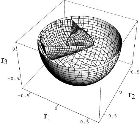
FIG. 2.: The Bloch sphere over the point $r_{+}=0.27$ and $r_{-}=0.1$ in ${\cal W}^{0}$. Innermost solid: triseparable states ${\cal T}$. Between ${\cal T}$ and outer sphere: the boundary of the biseparable states ${\cal B}_{1}$.

C States with Positive Partial Transpose

Holding the partition $1|23$ fixed we can compare the set of states with positive partial transpose with respect to the first subsystem (${\cal P}_{1}$) to ${\cal B}_{1}$. If Peres’ Criterion were valid in this case, we would have equality in ${\cal P}_{1}\supset{\cal B}_{1}$. It turns out that the inclusion is strict, but in several respects the criterion is amazingly good. To begin with, the intersections of both sets with two important hyperplanes coincide: namely (1) the $r_{-}=0$ plane (in particular, for three qubits), and (2) the $r_{2}=r_{3}=0$ plane, i.e. for states which are invariant under the $2\leftrightarrow 3$ interchange. In particular, the projections to the permutation invariant subset coincide, so no difference can be seen in Figure 1.

Despite this similarity the technique for computing ${\cal P}_{1}$ is completely different. The key is the observation that partial transposition in the first factor maps operators commuting with all unitaries $(U\otimes U\otimes U)$ to operators commuting with all unitaries of the form $(\overline{U}\otimes U\otimes U)$. Obviously, the latter set is again an algebra, which even happens to be isomorphic to the algebra $(U\otimes U\otimes U)$-invariant operators: two one-dimensional summands plus the $2\times 2$-matrices. Hence positivity of partial transposes can be decided along the same lines as in Criterion 1.

Criterion 4

Let $\rho\in{\cal W}$ be a density operator with expectations $r_{k}=\mathop{\rm tr}\nolimits(\rho R_{k})$, $k=+,-,1,2,3$. Then the partial transpose of $\rho$ with respect to the first tensor factor is positive, i.e. $\rho\in{\cal P}_{1}$, if and only if

$$s_{1}\equiv 1-r_{1}-5r_{-}-r_{+} \geq 0$$ (23)

$$s_{2}\equiv-1-r_{1}+r_{-}+5r_{+} \geq 0$$ (24)

$$\text{\em and}\qquad r_{2}^{2}+r_{3}^{2} \leq s_{1}s_{2}/3\;.$$ (25)

Note that condition (25) is exactly the same as the quadratic inequality in Criterion 3, Part(b). Therefore, we need not even provide a new plot for the set ${\cal P}_{1}$: In Figure 2, this set can be obtained simply by extending the quadratic surface, which wraps around ${\cal T}$, all the way to the boundary of the Bloch sphere. In other words, the difference between ${\cal B}_{1}$ and ${\cal P}_{1}$ is only that states in ${\cal B}_{1}$ have to satisfy an additional quadratic inequality, which is represented in Figure 2 by the surface tangent to the Bloch sphere.

REFERENCES

- [1] R. F. Werner, Phys. Rev. A 40, 4277 (1989).
- [2] W. Dür, J. I. Cirac, and R. Tarrach, Phys. Rev. Lett. 83, 3562 (1999).
- [3] A. Peres, Phys. Rev. Lett. 77, 1413 (1996).
- [4] H. Weyl, The Classical Groups, (Princeton University, 1946).