Double jumps and transition rates for two dipole-interacting atoms

Abstract

Cooperative effects in the fluorescence of two dipole-interacting atoms, with macroscopic quantum jumps (light and dark periods), are investigated. The transition rates between different intensity periods are calculated in closed form and are used to determine the rates of double jumps between periods of double intensity and dark periods, the mean duration of the three intensity periods and the mean rate of their occurrence. We predict, to our knowledge for the first time, cooperative effects for double jumps, for atomic distances from one and to ten wave lengths of the strong transition. The double jump rate, as a function of the atomic distance, can show oscillations of up to $30\%$ at distances of about a wave length, and oscillations are still noticeable at a distance of ten wave lengths. The cooperative effects of the quantities and their characteristic behavior turn out to be strongly dependent on the laser detuning.

I Introduction

The dipole-dipole interaction between two atoms can be understood through the exchange of virtual photons and depends on the transition dipole moment of the levels involved. It can be characterized by complex coupling constants, or by their real and imaginary parts, where the former affect decay constants and the latter lead to level shifts aga . Cooperative effects in the radiative behavior of atoms which may arise from their mutual dipole-dipole interaction have attracted considerable interest in the literature aga -Ho . Two of the present authors BeHe4 have investigated in detail the transition from anti-bunching to bunching with decreasing atomic distance for two dipole-dipole interacting two-level atoms.

The striking phenomenon of macroscopic quantum jumps (electron shelving or macroscopic dark and light periods) can occur for a multi-level system where the electron is essentially shelved for seconds or even minutes in a metastable state without photon emissions SauterL -HePle1 . For two such systems the fluorescence behavior would, without cooperative effects, be just the sum of the separate photon emissions, with dark periods of both atoms, light periods of a single atom and of two atoms. In Ref. Sauter the fluorescence intensity of three such ions in a Paul trap was measured and a large fraction of double or triple jumps was reported, i.e. jumps by two or three intensity steps within the short resolution time. This fraction was orders of magnitudes larger than that expected for independent ions. A quantitative explanation of such a large cooperative effect for distances of the order of ten wave lengths of the strong transition has been found to be difficult hendriks ; Java ; Aga88 ; Lawande89 ; Chun . Other experiments at larger distances and with different ions showed no cooperative effects Itano88 ; Thom .

Quite recently, two of the present authors BeHe5 investigated for two such systems cooperative effects in the mean duration, $T_{0}$, $T_{1}$, and $T_{2}$, of the dark, single-intensity, and double-intensity periods, respectively. This was done by simulations for two atoms in a $V$ configuration. The mean duration of the single- and double-intensity periods depended sensitively on the dipole-dipole interaction and thus on the atomic distance $r$. They exhibited noticeable oscillations which decreased in amplitude when $r$ increased. These oscillations seemed to continue up to a distance of well over five wave lengths of the strong transition and they were opposite in phase with those of Re$\,C_{3}(r)$, where $\,C_{3}$ is the complex dipole-dipole coupling constant associated with the strong transitions.

In this paper we present an analytic approach to study cooperative effects for atoms with macroscopic quantum jumps. This is explained for two atoms, but is easily generalized. The approach is based on an explicit calculation of transition rates between the various intensity periods. From the transition rates all interesting statistical quantities can be determined, such as double jump rates and mean duration of different periods.

We predict, to our knowledge for the first time, cooperative effects in the double jumps of two dipole-dipole interacting atoms. These results are for atoms in the $V$ configuration (see Fig. 1) and are verified by simulations. As a function of the atomic distance, the double jump rates show marked oscillations, with a maximal difference of up to 30%, decreasing as $1/r$. Most surprising is a change in the oscillatory behavior of the double jump rate from in phase with Re$\,C_{3}(r)$ to opposite in phase when the detuning of the laser driving the weak atomic transition is increased. For the mean durations $T_{1}$ and $T_{2}$ there can be a change in behavior from opposite in phase to in phase with Re$\,C_{3}(r)$. Moreover, for a particular value of the detuning, which depends on the other parameters, the double jump rate becomes constant in $r$ and the cooperative effects disappear. This is true also for the mean period durations and for their mean occurrences, with different values of the detuning, though. Typically, for nonzero detuning the oscillation amplitudes do not exceed those found for zero detuning.

The experiments of Ref. Sauter exhibited extremely large cooperative effects, in fact up to three orders of magnitude. Since this was for a different atomic level configuration and for three ions in a trap our results do not apply directly. In principle, however, our analytic approach can be carried over to the experimental situation of Ref. Sauter , although the calculations become algebraically more involved and have not been carried out so far.

The plan of the paper is as follows. In Section II the fluorescence with its three different intensity periods is treated as a three-step telegraph process and the Bloch equations are used to derive the transition rates between the periods. In Sections III and IV expressions for the double jump rate and the mean duration of the three types of intensity periods are obtained by means of these transition rates. The results are compared with simulations in which photon intensities are obtained by averaging photon numbers over a small time window. It turns out that this data-smoothing procedure can affect the results, and we show how this can be corrected for quantitatively. A similar effect can also occur when photon detectors measure the intensity of light by averaging over a small time window. In the last section the results are discussed. It is suggested that the mean rate of double-intensity periods is an experimentally more easily accessible candidate for exhibiting cooperative effects arising from the dipole-dipole interaction.

II Transition rates

II.1 Prerequisites

We consider two atoms, at a fixed distance r, each a $V$ configuration as shown in Fig. 1.

Figure 1: V system with metastable level 2 and Einstein coefficient $A_{3}$ for level 3. $\Omega_{2}$ and $\Omega_{3}$ are the Rabi frequencies of the two lasers driving the weak 1-2 transition and the strong 1-3 transition, respectively.

We assume the laser radiation normal to this line, and for the Einstein coefficients, the Rabi frequencies and the detuning we assume the relations

$$\Omega_{2}\ll\Omega_{3}~{},~{}~{}\Omega_{2}\ll\Omega_{3}^{2}/A_{3},~{}~{}A_{2}\approx 0,~{}~{}\Delta_{3}=0,$$ (1)

$\Delta_{2}$ arbitrary. The Dicke states are defined as

$$|g\rangle = |1\rangle|1\rangle,~{}~{}~{}|e_{2}\rangle=|2\rangle|2\rangle,~{}~{}~{}|e_{3}\rangle=|3\rangle|3\rangle$$

$$|s_{jk}\rangle = \{|j\rangle|k\rangle+|j\rangle|k\rangle\}/\sqrt{2}$$

$$i|a_{jk}\rangle = \{|j\rangle|k\rangle-|j\rangle|k\rangle\}/\sqrt{2}$$

They are symmetric and antisymmetric, respectively, under permutation of the two atoms. The Dicke states and the possible transitions are displayed in Fig. 2.

Figure 2: Dicke states. Simple arrows denote decays. Solid and dashed double arrows denote strong and weak driving, respectively.

Solid single and double arrows indicate decay and strong driving by laser 3, respectively, while dashed double arrows indicate the weak driving by laser 2. For $\Omega_{2}=0$, i.e. with the dashed arrows absent, the states decompose into three non-connected subsets, namely $|e_{2}\rangle$, the four states of the inner ring and the four states of the outer ring in Fig. 2, and the subspaces spanned by these states will be denoted by dark, inner, and outer subspace, respectively. As in Ref. BeHe5 they will be associated in the following with the fluorescence periods of intensity 0, 1, and 2:

$${\rm dark~{}state} : |e_{2}\rangle$$ (2)

$${\rm inner~{}states~{}(intensity~{}1)} : |s_{12}\rangle,|s_{23}\rangle,|a_{12}\rangle,|a_{23}\rangle$$ (3)

$${\rm outer~{}states~{}(intensity~{}2)} : |g\rangle,|s_{13}\rangle,|e_{3}\rangle,|a_{13}\rangle$$ (4)

The weak laser will lead to slow transitions between the subspaces.

The Bloch equations can be written, with the conditional Hamiltonian $H_{\rm cond}$ and the reset operation $\cal R$ of Appendix A, in the compact form BeHe4 ; He

$$\dot{\rho}=-~{}\frac{\rm i}{\hbar}~{}[H_{{\rm cond}}\rho-\rho H^{\dagger}_{{\rm cond}}]+{\cal R}(\rho)~{}.$$ (5)

The operator $H_{\rm cond}$ is of the form

$$H_{\rm cond}=H_{\rm cond}^{0}+H_{\rm cond}^{1}(\Omega_{2})$$ (6)

where the operator $H_{\rm cond}^{0}$ depends on $\Omega_{3}$ and on the dipole-dipole coupling constant $C_{3}(r)$, while $H_{\rm cond}^{1}$ is linear in $\Omega_{2}$ and does not depend on $C_{3}$ and $\Omega_{3}$. The super-operator ${\cal R}$ depends on $C_{3}$.

II.2 Intensity periods and subspaces

For a single atom as in Fig. 1, with macroscopic light and dark periods, the stochastic sequence of individual photon emissions can be directly analyzed by the quantum jump approach HeWi ; Wi ; He ; HeSo ; MC ; QT ; PleKni , using the existence of different time scales. To high precision it yields a telegraph process and the transition rates between the periods BeHe1 ; BeHeSo . A more heuristic approach assumes that during a light period the density matrix of the atom lies in the subspace spanned by $|1\rangle$ and $|3\rangle$ and that during a dark period the state is given by $|2\rangle$ Cook . One can then use the Bloch equations to calculate the build-up, during a time $\Delta t$, of a population outside the respective subspace and obtains from this the probability of leaving the subspace. This probability is then interpreted as the transition probability from one period to the other. The results agree with those of the more microscopic quantum jump approach HeWi ; Wi ; HePle1 ; HePle2 .

This idea will be used here for two dipole-interacting $V$ systems. We associate each of the three types of fluorescence periods with one of the subspaces spanned by the states in Eq. (2) - (4) and model transitions between periods as transitions between the corresponding subspaces. Without dipole interaction this is the same assumption as for a single atom, and with the interaction it has been tested numerically in Ref. beige to hold as long as the atomic separation is larger than a third wavelength of the strong transition.

Thus, at a particular time $t_{0}$, the density matrix $\rho(t_{0})$ of the two atoms is assumed to lie in one of the subspaces. Then, during a short time $\Delta t$, satisfying

$$\Omega_{3}^{-1}\!,A_{3}^{-1}\ll\Delta t\ll\Omega_{2}^{-1},$$ (7)

the system will go over to a density matrix $\rho(t_{0}+\Delta t)$ which contains small populations in the other subspaces, due to the driving by $\Omega_{2}\!\neq\!0$. The time derivatives of these populations at $t_{0}+\Delta t$ give the transition rates to these subspaces because, as shown in Appendix B, they are independent of the particular choice of $\Delta t$ and of the particular density matrix $\rho(t_{0})$, as long as Eq. (7) is fulfilled. These rates can be interpreted as transition rates between corresponding intensity periods, just as in the one-atom case.

A straightforward calculation using Eq. (5) yields the exact relations

$$\frac{\rm d}{\rm dt}\sum_{\rm outer}\langle{\rm outer}|\rho|{\rm outer}\rangle$$ (8)

$$\hskip 4.30554pt=\Omega_{2}{\rm Im}\Big{\{}\sqrt{2}\langle s_{12}|\rho|g\rangle+\langle s_{23}|\rho|s_{13}\rangle+\langle a_{23}|\rho|a_{13}\rangle\Big{\}}$$

$$\frac{\rm d}{\rm dt}\langle e_{2}|\rho|e_{2}\rangle=\sqrt{2}\Omega_{2}{\rm Im}\langle s_{12}|\rho|e_{2}\rangle$$ (9)

$$\frac{\rm d}{\rm dt}\sum_{\rm inner}\langle{\rm inner}|\rho|{\rm inner}\rangle$$ (10)

$$\hskip 30.1388pt=-\frac{\rm d}{\rm dt}\Big{\{}\langle e_{2}|\rho|e_{2}\rangle+\sum_{\rm outer}\langle{\rm outer}|\rho|{\rm outer}\rangle\Big{\}}$$

where $|{\rm outer}\rangle$ stands for $|g\rangle$, $|s_{13}\rangle$, $|e_{3}\rangle$, $|a_{13}\rangle$ and $|{\rm inner}\rangle$ for $|s_{12}\rangle,|s_{23}\rangle,|a_{12}\rangle,|a_{23}\rangle$. Thus one has to calculate the coherences on the right-hand side at time $t_{0}+\Delta t$ to first order in $\Omega_{2}$, with the appropriate initial condition at time $t_{0}$, to obtain the transition rate to second order in $\Omega_{2}$.

If $\rho(t_{0})$ lies in one of the above subspaces then by time $t_{0}+\Delta t$ the system has reached a quasi-stationary state satisfying

$${\dot{\rho}}(t_{0}+\Delta t)=0~{}~{}~{}~{}~{}{\rm to~{}first~{}order~{}in~{}}\Omega_{2},$$ (11)

as shown in Appendix B. This is also true for a single atom and is the decisive equation.

To obtain from this the coherences to first order in $\Omega_{2}$ we write

$$\rho(t_{0}+\Delta t)=\rho^{0}+\rho^{1}+\cdots$$

where $\rho^{k}$ is of order $\Omega_{2}^{k}$. Putting $\dot{\rho}=0$ in Eq. (5) and inserting the expansion for $\rho$ one obtains in zeroth order

$$0 = -{{\rm i}\over\hbar}\left[H_{\rm cond}^{0}\rho^{0}-\rho^{0}H_{\rm cond}^{0\,\dagger}\right]+{\cal R}(\rho^{0})$$ (12)

and in first order in $\Omega_{2}$

$$0=-{{\rm i}\over\hbar}\left[H_{\rm cond}^{0}\rho^{1}-\rho^{1}H_{\rm cond}^{0\,\dagger}+H_{\rm cond}^{1}\rho^{0}-\rho^{0}H_{\rm cond}^{1\,\dagger}\right]$$ (13)

$$\hskip 167.91614pt+{\cal R}(\rho^{1}).$$

Thus $\rho^{0}$ is an equilibrium state for $\Omega_{2}=0$, taken to lie in the appropriate subspace. For the dark state and the subspace spanned by the inner states one has

$$\rho^{0}\equiv\rho^{0}_{\rm dark} = |e_{2}\rangle\langle e_{2}|$$ (14)

$$\rho^{0}\equiv\rho^{0}_{\rm inner}=\frac{1}{2}\big{\{}\rho_{{\rm ss}}^{(A)}\otimes|2\rangle\langle 2|+|2\rangle\langle 2|\otimes\rho_{{\rm ss}}^{(B)}\big{\}}$$ (15)

$$\hskip 51.6665pt=\frac{1}{4}\frac{A_{3}^{2}+\Omega_{3}^{2}}{A_{3}^{2}+2\Omega_{3}^{2}}\{|s_{12}\rangle\langle s_{12}|+|a_{12}\rangle\langle a_{12}|\}$$

$$\hskip 51.6665pt+\frac{1}{4}\frac{\Omega_{3}^{2}}{A_{3}^{2}+2\Omega_{3}^{2}}\{|s_{23}\rangle\langle s_{23}|+|a_{23}\rangle\langle a_{23}|\}$$

$$\hskip 12.91663pt+\frac{i}{2}\frac{\Omega_{3}A_{3}}{A_{3}^{2}+2\Omega_{3}^{2}}\{|s_{12}\rangle\langle s_{23}|-|a_{12}\rangle\langle a_{23}|\}+{\rm H.c.}$$

by symmetry, independently of $C_{3}$, where $\rho_{{\rm ss}}^{(A,B)}$ are the steady states of the individual atoms in the $1$-$3$ subspace (for $\Omega_{2}=0$ and $C_{3}=0$). For the subspace spanned by the outer states one calculates

$$\rho^{0}\equiv\rho^{0}_{\rm outer}\propto\Big{[}\big{\{}(A_{3}^{2}+\Omega_{3}^{2})^{2}+A_{3}^{2}\,|C_{3}|^{2}+2A_{3}^{3}\,{\rm Re}\,C_{3}\big{\}}|g\rangle\langle g|$$ (16)

$$\hskip 17.22217pt+\big{\{}i\sqrt{2}\,A_{3}\,\Omega_{3}\,(A_{3}^{2}+\Omega_{3}^{4}+A_{3}\,C_{3})|g\rangle\langle s_{13}|+{\rm H.c.}\big{\}}$$

$$\hskip 17.22217pt-\big{\{}A_{3}\,\Omega_{3}^{2}\,(A_{3}+C_{3})|g\rangle\langle e_{3}|+{\rm H.c.}\big{\}}$$

$$\hskip 17.22217pt+\Omega_{3}^{2}\,(2A_{3}^{2}+\Omega_{3}^{2})|s_{13}\rangle\langle s_{13}|+\Omega_{3}^{4}\,\big{\{}|e_{3}\rangle\langle e_{3}|+|a_{13}\rangle\langle a_{13}|\big{\}}$$

$$\hskip 17.22217pt+\big{\{}i\sqrt{2}\,A_{3}\,\Omega_{3}^{3}|s_{13}\rangle\langle e_{3}|+{\rm H.c.}\big{\}}\Big{]}$$

One checks that for $C_{3}=0$ this becomes $\rho^{0}_{\rm outer}\propto\rho_{{\rm ss}}^{(A)}\otimes\rho_{{\rm ss}}^{(B)}$, the expression for two independent atoms.

We will denote the transition rates between the subspaces by $p_{ij}$. Here $i,j=0,1,2$ refer to the dark, inner and outer subspace, respectively, (and thus to the corresponding intensities). The $p_{ij}$ will be determined to second order in $\Omega_{2}$. As expected, $p_{02}$ and $p_{20}$ will turn out to be zero.

II.3 Calculation of $p_{12}$

We start from $\rho^{0}=\rho^{0}_{\rm inner}$ in Eq. (15) as initial state. For the the transition rate $p_{12}$ to the outer subspace one needs, in view of Eq. (8), three coherences of $\rho^{1}$ between the inner and outer subspace. To obtain these we write $\{|x_{i}\rangle\}=\{|s_{12}\rangle,|s_{23}\rangle,|a_{12}\rangle,|a_{23}\rangle\}$ (inner states) and $\{|y_{j}\rangle\}=\{|g\rangle,|s_{13}\rangle,|e_{3}\rangle,|a_{13}\rangle\}$ (outer states) for the corresponding bases and decompose

$$\rho^{1} = \sum_{i,j}\rho_{ij}^{1}\,|x_{i}\rangle\langle y_{j}|+\rho_{ij}^{1*}\,|y_{j}\rangle\langle x_{i}|+{\rm other~{}terms}~{}.$$ (17)

Inserting this into Eq. (13) and taking matrix elements with $\langle x_{i_{0}}|$ on the left and $|y_{j_{0}}\rangle$ on the right gives

$$0 = \frac{i}{\hbar}\langle x_{i_{0}}|\rho^{0}_{\rm inner}H_{\rm cond}^{1\,\dagger}|y_{j_{0}}\rangle-\frac{i}{\hbar}\sum_{i}\rho_{ij_{0}}^{1}\,\langle x_{i_{0}}|H_{\rm cond}^{0}|x_{i}\rangle$$ (18)

$$+\frac{i}{\hbar}\sum_{j}\rho_{i_{0}j}^{1}\,\langle y_{j}|H_{\rm cond}^{0\,\dagger}|y_{j_{0}}\rangle$$

$$+\sum_{i,j}(A_{3}+{\rm Re}\,C_{3})\rho^{1}_{ij}\langle x_{i_{0}}|R_{+}|x_{i}\rangle\langle y_{j}|R_{+}^{\dagger}|y_{j_{0}}\rangle$$

$$+\sum_{i,j}(A_{3}-{\rm Re}\,C_{3})\rho^{1}_{ij}\langle x_{i_{0}}|R_{-}|x_{i}\rangle\langle y_{j}|R_{-}^{\dagger}|y_{j_{0}}\rangle~{}.$$

This is a system of 16 linear equations for the 16 coherences $\rho^{1}_{ij}$, of which only three are needed in Eq. (8). Due to the symmetry of $H_{\rm cond}$ and $R_{+}$ and antisymmetry of $R_{-}$ under the interchange of the two atoms, the system decouples. Taking for $|x_{i_{0}}\rangle$ and $|y_{j_{0}}\rangle$ either both symmetric or both antisymmetric states and putting the eight coherences into the column vector

$$\tilde{\bf\rho}\equiv(\rho_{s_{12}g}^{1},~{}\rho_{s_{12}s_{13}}^{1},~{}\rho_{s_{12}e_{3}}^{1},~{}\rho_{s_{23}g}^{1},~{}\rho_{s_{23}s_{13}}^{1},~{}\rho_{s_{23}e_{3}}^{1},~{}\rho_{a_{12}a_{13}}^{1},~{}\rho_{a_{23}a_{13}}^{1})^{T}$$ (19)

one obtains the equation

$$({\bf A}-i\Delta_{2}{\bf 1})\tilde{\bf\rho}={\bf a}_{1}$$ (20)

where

$${\bf A}=$$ (30)

$$\left[\begin{array}[]{cccccccc}0&-i\Omega_{3}/\sqrt{2}&0&i\Omega_{3}/2&-(A_{3}\!+\!{\rm Re}C_{3})/\sqrt{2}&0&0&({\rm Re}C_{3}\!-\!A_{3})/\sqrt{2}\\ -i\Omega_{3}/\sqrt{2}&(A_{3}\!+\!C_{3}^{\ast})/2&-i\Omega_{3}/\sqrt{2}&0&i\Omega_{3}/2&-(A_{3}\!+\!{\rm Re}C_{3})/\sqrt{2}&0&0\\ 0&-i\Omega_{3}/\sqrt{2}&A_{3}&0&0&i\Omega_{3}/2&0&0\\ i\Omega_{3}/2&0&0&A_{3}/2&-i\Omega_{3}/\sqrt{2}&0&0&0\\ 0&i\Omega_{3}/2&0&-i\Omega_{3}/\sqrt{2}&(A_{3}\!+\!C_{3}^{\ast}/2)&-i\Omega_{3}/\sqrt{2}&0&0\\ 0&0&i\Omega_{3}/2&0&-i\Omega_{3}/\sqrt{2}&3A_{3}/2&0&0\\ 0&0&0&0&0&-(A_{3}\!-\!{\rm Re}C_{3})/\sqrt{2}&(A_{3}\!-\!C_{3}^{\ast})/2&-i\Omega_{3}/2\\ 0&0&0&0&0&0&-i\Omega_{3}/2&(A_{3}\!-\!C_{3}^{\ast}/2)\end{array}\right]$$

$${\bf a}_{1}=\frac{i\Omega_{2}\Omega_{3}}{4(A_{3}^{2}+2\Omega_{3}^{2})}\left[\sqrt{2}\,\frac{\Omega_{3}^{2}+A_{3}^{2}}{\Omega_{3}},i\,A_{3},0,-i\sqrt{2}\,A_{3},\Omega_{3},0,-i\,A_{3},\Omega_{3}\right]^{T}.$$ (31)

Inverting the $8\times 8$ matrix ${{\bf A}-i\Delta_{2}{\bf 1}}$ by Maple yields $\tilde{\bf\rho}$ and the coherences. The result is complicated and not illuminating. Inserting the required coherences into Eq. (8) one obtains, to first order in Re$\,C_{3}$ and Im$\,C_{3}$ and to second order in $\Omega_{2}$,

$$p_{12}=\Omega_{2}^{2}\Big{\{}\frac{A_{3}\Omega_{3}^{2}}{\Omega_{3}^{4}-8\Delta_{2}^{2}\Omega_{3}^{2}+4A_{3}^{2}\Delta_{2}^{2}+16\Delta_{2}^{4}}$$ (32)

$$+{\rm Re\,}C_{3}(r)\frac{2A_{3}^{2}\Omega_{3}^{2}(\Omega_{3}^{4}\!-\!4A_{3}^{2}\Delta_{2}^{2}\!-\!16\Delta_{2}^{4})}{(A_{3}^{2}\!+\!2\Omega_{3}^{2})(\Omega_{3}^{4}\!-\!8\Delta_{2}^{2}\Omega_{3}^{2}\!+\!4A_{3}^{2}\Delta_{2}^{2}\!+\!16\Delta_{2}^{4})^{2}}\Big{\}}.$$

Note that only Re$\,C_{3}$ appears and that the terms linear in Im$\,C_{3}$ have canceled.

II.4 Calculation of $p_{10}$

To determine $p_{10}$ we use Eq. (9) and start again from $\rho^{0}=\rho^{0}_{\rm inner}$ as initial condition in Eq. (13), but now have to determine $\langle s_{12}|\rho^{1}|e_{2}\rangle$. Replacing $\{|y_{i}\rangle\}$ by $|e_{2}\rangle$ and choosing $|x_{i_{0}}\rangle=|s_{12}\rangle,~{}|s_{23}\rangle$ in Eq. (18), one obtains two inhomogeneous linear equations for $\langle s_{12}|\rho^{1}|e_{2}\rangle$ and $\langle s_{23}|\rho^{1}|e_{2}\rangle$. These equations do not depend on $C_{3}$, since $R_{\pm}$ and $R_{\pm}^{\dagger}$ vanish on $|e_{2}\rangle$ and since $C_{3}$ does not appear in the part of $H_{\rm cond}$ acting on the inner states. Therefore $\langle s_{12}|\rho^{1}|e_{2}\rangle$ and $\langle s_{23}|\rho^{1}|e_{2}\rangle$ are independent of $C_{3}$. By a simple calculation one obtains $\langle s_{12}|\rho^{1}|e_{2}\rangle$ and inserting this into Eq. (9) yields, to second order in $\Omega_{2}$,

$$p_{10}=\Omega_{2}^{2}\frac{A_{3}\Omega_{3}^{2}(A_{3}^{2}+4\Delta_{2}^{2})}{(A_{3}^{2}+2\Omega_{3}^{2})[(\Omega_{3}^{2}-4\Delta_{2}^{2})^{2}+4\Delta_{2}^{2}A_{3}^{2}]}~{}.$$ (33)

This is independent of $C_{3}$ and is the same as for two independent atoms, namely the transition rate for a single atom from a light to a dark period Wi .

II.5 Calculation of $p_{01}$

To determine $p_{01}$ we use Eq. (10). One also needs $\langle s_{12}|\rho^{1}|e_{2}\rangle$, as seen from Eq. (9), but in this case one has to start from $\rho^{0}=\rho^{0}_{\rm dark}$ as initial condition in Eq. (13). Therefore one obtains the same equations for $\langle s_{12}|\rho^{1}|e_{2}\rangle$ and $\langle s_{23}|\rho^{1}|e_{2}\rangle$ as before, except for the inhomogeneous part. One has independence of $C_{3}$ and easily solves for $\langle s_{12}|\rho^{1}|e_{2}\rangle$.

For the remaining coherences needed in Eq. (10), i.e. those in Eq. (8), one obtains the same form as in Eq. (20), with the same ${\bf A}$, but now with ${\bf a}_{1}=0$ since the term containing $\rho^{0}$ vanishes. Therefore these coherences vanish here and hence $p_{02}=0$. Physically this means that in our formulation of the problem there are no direct transitions from a dark period to a period of intensity 2.

From Eq. (10) one now obtains, to second order in $\Omega_{2}$,

$$p_{01}=2\Omega_{2}^{2}\frac{A_{3}\Omega_{3}^{2}}{(\Omega_{3}^{2}-4\Delta_{2}^{2})^{2}+4\Delta_{2}^{2}A_{3}^{2}}$$ (34)

This is independent of $C_{3}$ and is the same as for two independent atoms, namely twice the transition rate for a single atom from a dark to a light period.

II.6 Calculation of $p_{21}$

The transition rate $p_{21}$ is obtained from Eq. (10) and the required coherences are again those appearing in Eq. (8) and (9), now with $\rho^{0}=\rho^{0}_{\rm outer}$ as initial condition. For $\langle s_{12}|\rho^{1}|e_{2}\rangle$ and $\langle s_{23}|\rho^{1}|e_{2}\rangle$ one obtains the same two equations as before, except for the inhomogeneous part which now vanishes. Hence these two coherences vanish now and as a consequence $p_{20}=0$. Physically this means that in our formulation there are no direct transitions from a period of intensity 2 to a dark period. For the coherences in Eq. (19) one has the same equation as Eq. (20), with the same matrix ${\bf A}$ but with ${\bf a}_{1}$ replaced by

$${\bf a}_{2}=-i\Omega_{2}\Big{/}\big{\{}\sqrt{2}\left(4\,{\Omega_{3}}^{4}+4\,{\Omega_{3}}^{2}{{A_{3}}}^{2}+{A_{3}}^{2}{{{\rm Re}\,C_{3}}}^{2}+2\,{A_{3}}^{3}{{\rm Re}\,C_{3}}+{{A_{3}}}^{2}{{{\rm Im}\,C_{3}}}^{2}+{A_{3}}^{4}\right)\big{\}}$$ (35)

$$\times\left[\begin{array}[]{c}{{\Omega_{3}}}^{4}+2\,{{\Omega_{3}}}^{2}{{A_{3}}}^{2}+{{A_{3}}}^{2}{{\rm Re}\,C_{3}}^{2}+2\,{{A_{3}}}^{3}{\rm Re}\,C_{3}+{{A_{3}}}^{2}{{{\rm Im}\,C_{3}}}^{2}+{{A_{3}}}^{4}\\ \vskip 6.0pt plus 2.0pt minus 2.0pt\cr i{\Omega_{3}}\,\sqrt{2}{A_{3}}\,\left({{A_{3}}}^{2}+{A_{3}}\,{\rm Re}\,C_{3}+i{\rm Im}\,C_{3}\,{A_{3}}+{{\Omega_{3}}}^{2}\right)\\ \vskip 6.0pt plus 2.0pt minus 2.0pt\cr-{{\Omega_{3}}}^{2}\left({A_{3}}+{\rm Re}\,C_{3}+i{\rm Im}\,C_{3}\right){A_{3}}\\ \vskip 6.0pt plus 2.0pt minus 2.0pt\cr i{\Omega_{3}}\,{A_{3}}\,\left(-{{\Omega_{3}}}^{2}-{{A_{3}}}^{2}-{A_{3}}\,{\rm Re}\,C_{3}+i{\rm Im}\,C_{3}\,{A_{3}}\right)\\ \vskip 6.0pt plus 2.0pt minus 2.0pt\cr{{\Omega_{3}}}^{2}\left({{\Omega_{3}}}^{2}+2\,{{A_{3}}}^{2}\right)/\sqrt{2}\\ \vskip 6.0pt plus 2.0pt minus 2.0pt\cr i{{\Omega_{3}}}^{3}{A_{3}}\\ \vskip 6.0pt plus 2.0pt minus 2.0pt\cr 0\\ \vskip 6.0pt plus 2.0pt minus 2.0pt\cr{{\Omega_{3}}}^{4}/\sqrt{2}\end{array}\right]$$ (44)

Inserting the resulting coherences into Eq. (10) gives, to first order in Re$\,C_{3}$ and ${\rm Im}\,C_{3}$ and to second order in $\Omega_{2}$,

$$p_{21}=\Omega_{2}^{2}\Big{\{}\frac{2A_{3}\Omega_{3}^{2}(A_{3}^{2}+4\Delta_{2}^{2})}{(\Omega_{3}^{4}-8\Delta_{2}^{2}\Omega_{3}^{2}+16\Delta_{2}^{4}+4A_{3}^{2}\Delta_{2}^{2})(A_{3}^{2}+2\Omega_{3}^{2})}$$ (45)

$$\hskip 4.30554pt+{\rm Re\,}C_{3}(r)\,\frac{4A_{3}^{2}\Omega_{3}^{2}(A_{3}^{4}\Omega_{3}^{4}+4A_{3}^{2}\Omega_{3}^{6}-12A_{3}^{2}\Delta_{2}^{2}\Omega_{3}^{4}-64A_{3}^{2}\Delta_{2}^{6}-4A_{3}^{6}\Delta_{2}^{2}-32A_{3}^{4}\Delta_{2}^{4}-64\Delta_{2}^{4}\Omega_{3}^{4}+16\Delta_{2}^{2}\Omega_{3}^{6})}{(A_{3}^{2}+2\Omega_{3}^{2})^{3}(\Omega_{3}^{4}-8\Delta_{2}^{2}\Omega_{3}^{2}+4A_{3}^{2}\Delta_{2}^{2}+16\Delta_{2}^{4})^{2}}\Big{\}}$$

where again the terms containing Im$\,C_{3}$ have canceled.

II.7 Discussion.

If one computes the coherences in Eqs. (8) and (10) to second order in $C_{3}$ one obtains $p_{12}$ and $p_{21}$ to second order in $\,C_{3}$. The resulting expressions are not enlightening and therefore not given here, but they do depend on $({\rm Im}\,C_{3})^{2}$. Fig. 3 shows how small the second-order dipole-dipole contribution to $p_{21}$ is for the parameters of the simulations and for distances larger than half a wave length.

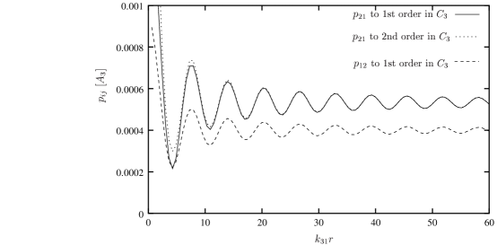
Figure 3: Transition probabilities $p_{21}$ to first and second order in $C_{3}$ and $p_{21}$ to first order, for $\Omega_{3}\!=\!0.5A_{3}$, $\Omega_{2}\!=\!0.01A_{3}$, zero detuning. The contribution to $p_{21}$ arising from the second order in $C_{3}$ is small.

For smaller distances the results are probably not applicable anyway, as discussed in Ref. BeHe5 .

For $\Delta_{2}=0$ the rates $p_{12}$ and $p_{21}$ simplify to

$$p_{12} = \Omega_{2}^{2}\Big{\{}\frac{A_{3}}{\Omega_{3}^{2}}+{\rm Re\,}C_{3}(r)\,\frac{2A_{3}^{2}}{\Omega_{3}^{2}(A_{3}^{2}+2\Omega_{3}^{2})}\Big{\}}$$ (46)

$$p_{21}=\Omega_{2}^{2}\Big{\{}\frac{2A_{3}^{3}}{\Omega_{3}^{2}(A_{3}^{2}\!+\!2\Omega_{3}^{2})}+$$ (47)

$$\hskip 86.11084pt{\rm Re\,}C_{3}(r)\,\frac{4A_{3}^{4}(A_{3}^{2}\!+\!4\Omega_{3}^{2})}{\Omega_{3}^{2}(A_{3}^{2}\!+\!2\Omega_{3}^{2})^{3}}\Big{\}}$$

and one sees that the coefficients of the Re$\,C_{3}$ term in Eqs. (46) and (47) are positive. For $\Delta_{2}=0$, therefore, $p_{12}$ and $p_{21}$ vary with the atomic distance in phase with Re$\,C_{3}$. For $\Delta_{2}\neq 0$, however, the coefficients of Re$\,C_{3}$ in Eqs. (32) or (45) can become zero or negative. In the first case $p_{12}$ or $p_{21}$ become constant in $r$, while in the second case they vary opposite in phase to Re$\,C_{3}$.

It will be shown in the next sections that this dependence of $p_{12}$ and $p_{21}$ on the detuning of the weak laser entails a corresponding behavior of the double jump rate and an opposite behavior of the mean durations $T_{1}$ and $T_{2}$. This opposite behavior of $T_{1}$ and $T_{2}$ is easy to understand since they are related to the inverse of the transition rates.

III Double jumps: Comparison of simulations with theory

A double jump is defined as a transition from a double-intensity period to dark period, or vice versa, within a prescribed time interval $\Delta T_{\rm DJ}$. Now, to distinguish different periods in experiments and in simulations one has to use an average photon intensity, obtained e.g. by means of averaging over a time window. This window has to be large enough to contain enough emissions, but must not be too large in order not to overlook too many short periods. Our simulations employ a procedure similar to that in Ref. BeHe5 and use a moving window window of fixed width, denoted by $\Delta T_{\rm w}$. The time interval $\Delta T_{\rm DJ}$ should be larger than $\Delta T_{\rm w}$.

We consider the fluorescence periods as a telegraph process with three steps and use the $p_{ij}$ of the last section as transition rates. At first the influence of the averaging window $T_{\rm w}$ will be neglected.

The rate of downward double jumps is obtained as follows. For $i$ = 0, 1, 2, let $n_{i}$ be the mean number of periods of intensity $i$ per unit time. For a long path of length $T$ the total number of periods of intensity $i$ is then $N_{i}(T)=n_{i}T$. At the end of each period of intensity 2 there begins a period of intensity 1, and the probability for this period of intensity 1 to be shorter than $\Delta T_{\rm DJ}$ is given by

$$1-\exp\{-(p_{10}+p_{12})\Delta T_{\rm DJ}\}.$$

At the end of a period of intensity 1 the branching ratio for a transition to a period of intensity 0 is $p_{10}/(p_{10}+p_{12})$. Thus during time $T$ the total number of such downward double jumps, denoted by $N^{20}_{\rm DJ}(T)$, is

$$N^{20}_{\rm DJ}(T)\!=\!N_{2}(T)\frac{p_{10}}{(p_{10}\!+\!p_{12})}\Big{\{}1\!-\exp\{-(p_{10}\!+\!p_{12})\Delta T_{\rm DJ}\}\Big{\}}$$

and therefore the rate, $n^{20}_{\rm DJ}$, of downward double jumps within $\Delta T_{\rm DJ}$ is

$$n^{20}_{\rm DJ}\!=\!n_{2}\frac{p_{10}}{(p_{10}\!+\!p_{12})}\Big{\{}1\!-\exp\{-(p_{10}+p_{12})\Delta T_{\rm DJ}\}\Big{\}}.$$ (48)

In a similar way one finds that the rate, $n^{02}_{\rm DJ}$, of upward double jumps within $\Delta T_{\rm DJ}$ is

$$n^{02}_{\rm DJ}\!=\!n_{0}\frac{p_{12}}{(p_{10}\!+\!p_{12})}\Big{\{}1\!-\exp\{-(p_{10}+p_{12})\Delta T_{\rm DJ}\}\Big{\}}.$$ (49)

It remains to determine $n_{0}$ and $n_{2}$. Since a period of intensity 1 ends with a transition to a period of either intensity 0 or intensity 2 one has, with the respective branching ratios,

$$n_{0}=\frac{p_{10}}{p_{10}+p_{12}}n_{1}$$ (50)

$$n_{2}=\frac{p_{12}}{p_{10}+p_{12}}n_{1}.$$ (51)

If one denotes by $T_{i}$ the mean durations of a period of intensity $i$, one has

$$\sum_{i=0}^{2}n_{i}T_{i}=1.$$ (52)

Moreover, one has

$$T_{0}=1/p_{01},~{}~{}~{}~{}~{}T_{1}=1/(p_{10}+p_{12}),~{}~{}~{}~{}~{}T_{2}=1/p_{21}$$ (53)

and this then gives

$$n_{0}=\frac{p_{01}p_{21}}{p_{01}p_{21}+p_{21}p_{10}+p_{01}p_{12}}p_{10}$$ (54)

$$n_{2}=\frac{p_{01}p_{21}}{p_{01}p_{21}+p_{21}p_{10}+p_{01}p_{12}}p_{21}.$$ (55)

From this, together with Eqs. (48) and (49), one sees immediately that the rates of upward and downward double jumps are equal,

$$n^{02}_{\rm DJ}=n^{20}_{\rm DJ}.$$ (56)

This fact was also observed in the simulations. The combined number of double jumps therefore equals

$$n_{\rm DJ}\equiv n^{02}_{\rm DJ}+n^{20}_{\rm DJ}$$ (57)

$$\hskip 21.52771pt=2\frac{p_{01}p_{10}p_{12}p_{21}}{(p_{01}p_{21}+p_{21}p_{10}+p_{01}p_{12})(p_{01}+p_{12})}$$

$$\hskip 55.97205pt\times\Big{\{}1-\exp\{-(p_{10}+p_{12})\Delta T_{\rm DJ}\}\Big{\}}.$$

For $\Delta T_{\rm DJ}\ll T_{1}$ and by expanding the exponential, this gives for the combined double jump rate, without correction for the averaging window,

$$n_{\rm DJ}=2\frac{p_{01}p_{10}p_{12}p_{21}}{p_{01}p_{21}+p_{21}p_{10}+p_{01}p_{12}}\Delta T_{\rm DJ}.$$ (58)

Fig. 4 shows a comparison of this result with data from the simulations.

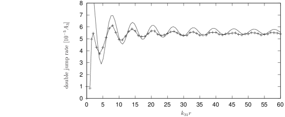
Figure 4: Double jump rates.  Simulation   $+++$ ,  theory   $-\!\!\!\!-\!\!\!-\!\!\!-$    uncorrected for averaging window ($\Omega_{3}\!=\!0.5~{}A_{3}$, $\Omega_{2}\!=\!0.01~{}A_{3}$, zero detuning).

Except for atomic distances less than about three quarters of the wave length of the strong transition the agreement appears as quite reasonable, and the disagreement for small distances is not unexpected since there the intensities start to decrease and a description by a telegraph process may be no longer a good approximation, as pointed out in Ref. BeHe5 . But one observes that the theoretical result is systematically above the simulated curve. This seeming disagreement, however, is easily explained and can be taken care of as follows.

III.1 Corrections for averaging window

We recall that the simulated data were obtained by averaging the numerical photon emission times with a moving window of length $\Delta T_{\rm w}$. Then, roughly, periods which are shorter than about two thirds of the window length are overlooked, and therefore the number of recorded (or observed) periods of type 2, which enters Eq. (48), is smaller than that given by Eq. (55). The recorded or observed number is denoted by $n_{2,\rm cor}$. It is approximately given by

$$n_{2,\rm cor}=n_{2}\exp\{-p_{21}\frac{2}{3}\Delta T_{\rm w}\},$$ (59)

and this expression should be inserted into Eq. (48) for $n_{2}$. In this way one obtains the corrected theoretical curve in Fig. 5.

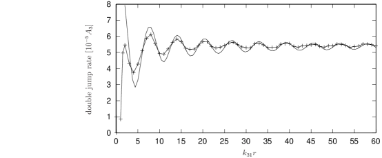
Figure 5: As in Fig 4 , but theory corrected for averaging window.

The curve changes very little if instead of two thirds one takes 60% or 70% of $\Delta T_{\rm w}$. It is seen that the agreement with the simulated data is much improved for distances greater than three quarters of a wave length of the strong transition.

It still appears, however, that the oscillation amplitudes of the theoretical curve are somewhat larger than those of the simulated curve. This is again understandable as an effect of the averaging procedure. In the simulations it was noticed numerically that the $r$ dependence of the double jump rate depended somewhat on the length of the averaging window $T_{\rm w}$ and distinct features tended to be somewhat washed out for larger $\Delta T_{\rm w}$, in particular the oscillation amplitudes of the simulated data decreased with the length of the averaging window. A larger $\Delta T_{\rm w}$ gave a smoother intensity curve, but made the determination of the transition times between different periods more difficult, while a shorter averaging window introduced more noise. We found the use of $\Delta T_{\rm w}=114~{}A_{3}^{-1}$ to be a good compromise. If it were possible to choose smaller averaging window the amplitudes should increase, as predicted by the theory.

III.2 Detuning

One can explicitly insert the expressions for $p_{ij}$ of the last section into Eq. (58), but the result becomes unwieldy. One can show that in an expansion of Eq. (58) with respect to Re$\,C_{3}$ to first order the coefficient of Re$\,C_{3}$ is positive for zero detuning. This implies that the double jump rate is in phase with Re$\,C_{3}(r)$ for the atomic distances under consideration and for zero detuning. For increasing detuning the double jump rate can become constant in $r$ and then change its oscillatory behavior to that of $-$Re$\,C_{3}$. An example for the latter is shown in Fig. 6.

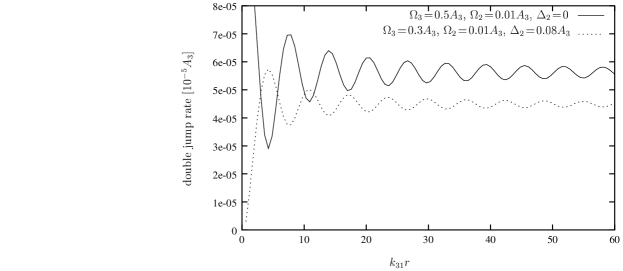
Figure 6: Changed oscillatory behavior of the double jump rate for increased detuning of the weak driving (uncorrected for averaging window).

IV Duration of fluorescence periods: Effect of averaging window

The mean durations, $T_{0}$, $T_{1}$, and $T_{2}$, of the three periods were investigated for cooperative effects in Ref. BeHe5 by simulations with averaging windows at discrete times. Here we have performed similar simulations with a moving averaging window. It turns out that both the present and the previous simulation for $T_{i}$ are about 15% higher than those predicted by Eq. (53), using the expressions for $p_{ij}$ of Section II and without correcting for the use of the averaging window due to which short periods are not recorded. We will now show how this can be taken into account in the theory.

As in Section III we consider a three-step telegraph process with periods of type 0, 1, and 2, whose mean durations are denoted by $T_{0}$, $T_{1}$, and $T_{2}$, respectively. We assume that periods of length $\Delta\tau$ or less are not recorded. Fig. 7 shows periods of type 1 which are interrupted by a short period of type 0 and 2, respectively.

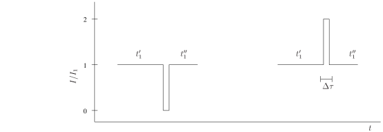
Figure 7: If periods of length $\Delta\tau$ or less are overlooked then the distribution of the periods is changed.

If the respective short periods are not recorded, then the two periods of type 1 in the left part of the figure are recorded as a single longer period, and similarly for the right part of the figure. This leads to an apparent decrease of shorter periods of type 1 and to a corresponding increase of longer periods.

To make this quantitative we put $\lambda_{i}\equiv 1/T_{i}$ and denote the number per unit time of periods of type $i$, whose duration is less than $\Delta\tau$, by $n_{i}^{\Delta\tau}$, i.e.

$$n_{i}^{\Delta\tau}=n_{i}\Big{\{}1-\exp\{-\lambda_{i}\Delta\tau\}\Big{\}}.$$ (60)

Per unit time, one has $n_{0}^{\Delta\tau}$ occurrences of the situation in the left part of Fig. 7 and $n_{2}^{\Delta\tau}$ occurrences of that in the right part. The probability for one of the periods of type 1 in the left or right part of Fig. 7 to have a length lying in the time interval $(t_{1},t_{1}+dt_{1})$ is $2\lambda_{1}\exp\{-\lambda_{1}t_{1}\}dt_{1}$, where the factor of 2 comes from the two possible situations. Therefore, the recorded number, per unit time, of periods of type 1 with duration in $(t_{1},t_{1}+dt_{1})$ is changed (decreased) by

$$2(n_{0}^{\Delta\tau}+n_{2}^{\Delta\tau})\lambda_{1}\exp\{-\lambda_{1}t_{1}\}dt_{1}.$$ (61)

Similarly, the apparent increase of the number, per unit time, of periods of type 1 with duration in $(t_{1},t_{1}+dt_{1})$ is, by Fig. 7,

$$(n_{0}^{\Delta\tau}+n_{2}^{\Delta\tau})~{}~{}~{}~{}~{}~{}\int\!\!\!\!\!\!\!\!\!\!\int\limits_{t_{1}\leq t_{1}^{\prime}+t_{1}^{\prime\prime}\leq t_{1}+dt_{1}}dt_{1}^{\prime}dt_{1}^{\prime\prime}$$ (62)

$$\hskip 68.88867pt\times\lambda_{1}\exp\{-\lambda_{1}t_{1}^{\prime}\}\lambda_{1}\exp\{-\lambda_{1}t_{1}^{\prime\prime}\}$$

$$\hskip 51.6665pt=(n_{0}^{\Delta\tau}+n_{2}^{\Delta\tau})\lambda_{1}^{2}t_{1}\exp\{-\lambda_{1}t_{1}\}dt_{1}.$$

Denoting by $\nu_{1\rm rec}(t_{1})dt_{1}$ the actually recorded number, per unit time, of periods of type 1 with duration in $(t_{1},t_{1}+dt_{1})$ one obtains from the two previous expressions

$$\nu_{1\rm rec}(t_{1})dt_{1}=n_{1}\lambda_{1}\exp\{-\lambda_{1}t_{1}\}dt_{1}$$ (63)

$$\hskip 17.22217pt+(n_{0}^{\Delta\tau}+n_{2}^{\Delta\tau})(\lambda_{1}^{2}t_{1}-2\lambda_{1})\exp\{-\lambda_{1}t_{1}\}dt_{1}.$$

The average duration of the recorded periods of type 1 will be denoted by $T_{1,\rm cor}$, and it is given by

$$T_{1,\rm cor}=\int_{\Delta\tau}^{\infty}dt_{1}\,t_{1}\nu_{1\rm rec}(t_{1})\bigg{/}\int_{\Delta\tau}^{\infty}dt_{1}\nu_{1\rm rec}(t_{1}).$$ (64)

Using Eq. (63) for $\nu_{1\rm rec}(t_{1})$ one obtains, after an elementary calculation and for $\Delta\tau$ satisfying $\Delta\tau/T_{1}\ll 1$,

$$T_{1,\rm cor}=\frac{1}{p_{10}+p_{12}}+\Delta\tau\left\{1+\frac{p_{01}p_{10}+p_{12}p_{21}}{(p_{10}+p_{12})^{2}}\right\}.$$ (65)

The first term is the ideal theoretical value, $T_{1}$, and the remainder is the correction due to non-recorded short periods. In a similar way one obtains

$$T_{0,\rm cor}=\frac{1}{p_{01}}+\Delta\tau\left\{1+\frac{p_{10}}{p_{01}}\right\}$$ (66)

$$T_{2,\rm cor}=\frac{1}{p_{21}}+\Delta\tau\left\{1+\frac{p_{12}}{p_{21}}\right\}$$ (67)

where again the respective first terms are the ideal values, $T_{0}$ and $T_{2}$.

To compare this with simulated data, obtained with a moving averaging window of length $\Delta T_{\rm w}=247~{}A_{3}^{-1}$, we have taken $\Delta\tau=\frac{2}{3}\Delta T_{\rm w}$, as in the previous section, and have plotted the results together with the simulated data in Fig. 8.

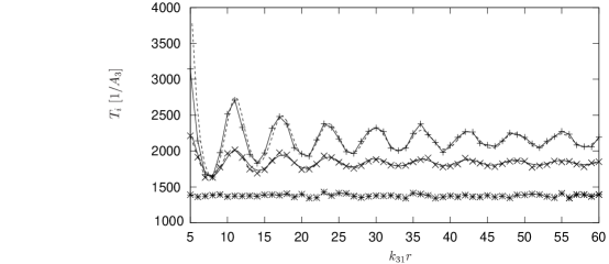
Figure 8: Mean duration of fluorescence periods. Simulation: $T_{2}$   $+++$,  $T_{1}$   $\times\times\times$,  $T_{0}$   $\ast\ast\ast$. Theory: $T_{2}$   $---$,  $T_{1}$   $-\!\!\!\!-\!\!\!-\!\!\!-$,  $T_{0}$   $....$    corrected for averaging window ($\Omega_{3}\!=\!0.5~{}A_{3}$, $\Omega_{2}\!=\!0.01~{}A_{3}$, zero detuning).

The agreement is very good. Quite generally, for zero detuning the oscillations of $T_{1}$ and $T_{2}$ are opposite in phase to those of Re$\,C_{3}(r)$, as already noted at the end of Section II. As in the case of the double jump rate, $T_{1}$ and $T_{2}$ can become constant in $r$ for particular values of the detuning (different for $T_{1}$ and $T_{2}$ ), and then change to a behavior in phase with Re$\,C_{3}(r)$.

The above approach of taking the averaging window into account works for the following reason. For a single atom with macroscopic dark periods it is known that the emission of photons is describable, to high accuracy, by an underlying two-step telegraph process. For two independent atoms with macroscopic dark periods the emissions are therefore described by an underlying three-step telegraph process. For two atoms interacting by a weak dipole-dipole interaction the actual emission process of photons should therefore still have, at least approximately, an underlying three-step telegraph process. What we have done above is replacing the actual emission process by this underlying three-step telegraph process and then incorporating the averaging window by taking into account the influence of the overlooked short periods on the statistics.

V Discussion of results

We have investigated cooperative effects in the fluorescence of two dipole-dipole interacting atoms in a $V$ configuration. One of the excited states of the $V$ configuration is assumed to be metastable, i.e. with a weak transition to the ground state. When driven by two lasers, a single such configuration exhibits macroscopic dark periods and periods of fixed intensity, like a two-step telegraph process. A system of two such atoms exhibits three fluorescence types, i.e. dark periods and periods of single and double intensity, like a three-step telegraph process. For large atomic distances, when the dipole-dipole interaction is negligible, the total fluorescence just consists of the sum of the individual atomic contributions. We have shown that for smaller atomic distances the fluorescence modified by the dipole-dipole interaction which depends on the atomic distance $r$. In particular we have, to our knowledge for the first time, explicitly demonstrated cooperative effects in the rate of double jumps from a period of double intensity to a dark period or vice versa, both analytically and by simulations.

By means of an analytical theory we have obtained the r-dependent transition rates , $p_{ij}$, between the three intensity periods. These were then used to calculate the rate of double jumps and in the mean period durations $T_{0},T_{1},$ and $T_{2}$. When comparing with the simulations it turned out that one had to take into account the averaging window used for obtaining an intensity curve from the individual photon emissions. With this the agreement between simulation and analytic theory became excellent.

For zero laser detuning, for which the simulations were performed, the double jump rates are in phase with and $T_{1}$ and $T_{2}$ opposite in phase to Re$\,C_{3}(r)$. The theoretical expressions, however, allow general detuning, $\Delta_{2}$, of the laser which drives the weak transition. It has been shown that for a particular $\Delta_{2}$, which depends on the other parameters, the double jump rate becomes constant and, for larger $\Delta_{2}$, varies opposite in phase to Re$\,C_{3}(r)$. A similar change of characteristic behavior also occurs for $T_{1}$ and $T_{2}$, for different values of $\Delta_{2}$ though. The amplitude of the oscillations with the atomic distance remain in the same region of magnitude as for zero detuning. As pointed out in Ref. BeHe5 , a dependence of the oscillations on Re$\,C_{3}(r)$ is not unexpected since Re$\,C_{3}(r)$ affects the decay rates of the excited Dicke states of the combined system. But an intuitive argument why the above change of behavior occurs for increased detuning is at present not apparent.

We have pointed out in Section III that there is another statistical property of the fluorescence which can serve as an indicator of the influence of the dipole-dipole interaction and which is probably not too difficult to determine experimentally. This quantity is the rate with which fluorescence periods of definite type occur, in particular the rate of periods with double intensity. Our theoretical results show that this rate behaves similar to the double jump rate, as regards the variation with the atomic distance, and an example is shown in Fig. 9.

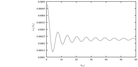
Figure 9: The theoretical rate, $n_{2}$, of double intensity periods per unit time shows distance-dependent cooperative effects ($\Omega_{3}\!=\!0.5~{}A_{3}$, $\Omega_{2}\!=\!0.01~{}A_{3}$, zero detuning).

This quantity is probably much easier to measure than the double jump rate or the mean duration $T_{2}$.

Our theoretical approach can be carried over to other level configurations and to more than two atoms. For given parameters the evaluation should be not too difficult. If, however, one is interested in closed algebraic expressions the effort will increase considerably with the number of atoms. In particular, it would be interesting to apply our approach to the situation of the experiment of Ref. Sauter with its different level configuration and its three ions in the trap.

Appendix A Dipole-dipole interaction in the Bloch equations

The dipole-dipole interaction enters the Bloch equations through $r$-dependent complex coupling constants (cf. Ref. BeHe5 )

$$C_{j}={3A_{j}\over 2}\,{\rm e}^{ik_{j1}r}\Bigg{[}{1\over{i}k_{j1}r}\left(1-\cos^{2}\vartheta_{j}\right)$$ (68)

$$\hskip 21.52771pt+\left({1\over(k_{j1}r)^{2}}-{1\over i(k_{j1}r)^{3}}\right)\left(1-3\cos^{2}\vartheta_{j}\right)\Bigg{]}.$$

Here $\vartheta_{j}$ is the angle between the transition dipole moment ${\bf D}_{1j}$ and the line connecting the atoms and $k_{j1}=2\pi/\lambda_{j1}$, where $\lambda_{j1}$ is the wavelength of the j-1 transition for an atom. For $A_{2}\approx 0$ one has $C_{2}\approx 0$. Thus one can neglect the dipole interaction when one atom is in state $|2\rangle$. The dependence of $C_{3}$ on $r$ is maximal for $\vartheta_{3}=\pi/2$ and the corresponding $C_{3}$ is plotted in Fig. 10.

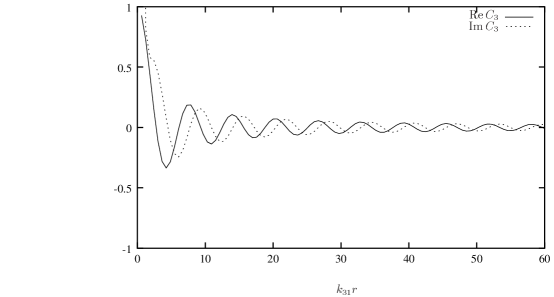
Figure 10: The complex dipole-dipole coupling constant $C_{3}$ for the strong transition as a function of the atomic distance.

For atomic distances greater than about three quarters of a wave length of the strong transition, $|C_{3}|$ is less than $0.2\,A_{3}$, but for smaller distances Re$\,C_{3}$ approaches $A_{3}$ and Im$\,C_{3}$ diverges.

The reset operation $\cal R$ and $H_{\rm cond}$ are given by the same expressions as in Ref. BeHe5 , except for the detuning. One has

$${\cal R}(\rho)\!=\!\left(A_{3}\!+\!{\rm Re}\,C_{3}\right)R_{+}\rho R^{\dagger}_{+}\!+\!\left(A_{3}\!-\!{\rm Re}\,C_{3}\right)R_{-}\rho R_{-}^{\dagger}$$ (69)

where

$$R_{+} = \left(S_{13}^{-}+S_{23}^{-}\right)/\sqrt{2}$$

$$= |g\rangle\langle s_{13}|\!+\!|s_{13}\rangle\langle e_{3}|+\big{(}|s_{12}\rangle\langle s_{23}|\!-\!|a_{12}\rangle\langle a_{23}|\big{)}/\sqrt{2},$$

$$R_{-} = \left(S_{13}^{-}-S_{23}^{-}\right)/\sqrt{2}$$ (70)

$$= |g\rangle\langle a_{13}|\!+\!|a_{13}\rangle\langle e_{3}|\!+\!\big{(}|s_{12}\rangle\langle a_{23}|\!+\!|a_{12}\rangle\langle s_{23}|\big{)}/\sqrt{2}.$$

The summands in Eq. (6) are given by

$$H^{0}_{\rm cond} = {\hbar\over 2i}\,\Big{[}A_{3}\,\big{(}|s_{23}\rangle\langle s_{23}|+|a_{23}\rangle\langle a_{23}|\big{)}+(A_{3}+C_{3})|s_{13}\rangle\langle s_{13}|+(A_{3}-C_{3})|a_{13}\rangle\langle a_{13}|+2A_{3}\,|e_{3}\rangle\langle e_{3}|\Big{]}$$ (71)

$$\hskip 8.61108pt+{\hbar\over 2}\Big{[}\sqrt{2}\Omega_{3}\big{(}|g\rangle\langle s_{13}|+|s_{13}\rangle\langle e_{3}|\big{)}+\Omega_{3}\big{(}|s_{12}\rangle\langle s_{23}|-|a_{12}\rangle\langle a_{23}|\big{)}+{\rm H.c.}\Big{]}$$

$$\hskip 21.52771pt-\hbar\Delta_{2}\Big{[}2|e_{2}\rangle\langle e_{2}|+|s_{12}\rangle\langle s_{12}|+|a_{12}\rangle\langle a_{12}|+|s_{23}\rangle\langle s_{23}|+|a_{23}\rangle\langle a_{23}|\Big{]}$$

$$H_{\rm cond}^{1}(\Omega_{2})={\hbar\over 2}\Big{[}\sqrt{2}\Omega_{2}\big{(}|g\rangle\langle s_{12}|+|s_{12}\rangle\langle e_{2}|\big{)}+\Omega_{2}\big{(}|s_{13}\rangle\langle s_{23}|+|a_{13}\rangle\langle a_{23}|\big{)}+{\rm H.c.}\Big{]}$$ (72)

From Eq. (71) one sees that Re$\,C_{3}$ changes the spontaneous decay rates and that Im$\,C_{3}$ leads to level shifts. Therefore, for small $r$, the decay rate of $|a_{13}\rangle$ approaches 0 in this case and the large level shifts cause a decrease of fluorescence associated with the levels $|s_{13}\rangle$ and $|a_{13}\rangle$.

Appendix B calculation of $\rho(t_{0}+\Delta t)$ to first order in $\Omega_{2}$

We write the Bloch equations of Eq. (5) in the form

$$\dot{\rho}={\cal L}\rho$$ (73)

where the Liouvillean ${\cal L}\equiv{\cal L}(A_{3},\Omega_{3},\Delta_{2},C_{3},\Omega_{2})$, a super-operator, can be read off from Eqs. (5) and (69) - (72). One can decompose ${\cal L}$ as

$${\cal L}={\cal L}_{0}+{\cal L}_{\Omega_{2}}$$ (74)

where ${\cal L}_{0}={\cal L}(A_{3},\Omega_{3},\Delta_{2},C_{3},0)$ and ${\cal L}_{\Omega_{2}}\rho=-{\rm i}[H_{\rm cond}^{1}(\Omega_{2}),\rho]/\hbar$. We note that $H_{\rm cond}^{1}(\Omega_{2})$ is Hermitian and that ${\cal L}_{0}$ can be considered as a Liouvillean of Bloch equations. Choosing an initial density matrix $\rho(t_{0})$ lying in one of the subspaces in Eqs. (2) - (4) one obtains, to first order in $\Omega_{2}$,

$$\rho(t_{0}+\Delta t) = e^{{\cal L}\Delta t}\rho(t_{0})$$ (75)

$$= e^{{\cal L}_{0}\Delta t}\rho(t_{0})$$

$$\hskip 12.91663pt+\int_{0}^{\Delta t}d\tau e^{{\cal L}_{0}(\Delta t-\tau)}{\cal L}_{\Omega_{2}}e^{{\cal L}_{0}\tau}\rho(t_{0}),$$

just as with usual quantum mechanical perturbation theory in the interaction picture. Now we use the fact that ${\cal L}_{0}$, as a Liouvillean of Bloch equations, has an eigenvalue $0$ (corresponding to steady states) and eigenvalues with negative real parts of the order of $\Omega_{3}$ and $A_{3}$. Therefore, if $\Delta t$ satisfies Eq. (7), the first term on the right-hand side of Eq. (75) gives one of the equilibrium states, $\rho^{0}$, of ${\cal L}_{0}$ given in Eqs. (14) - (16), to high accuracy, while the term $e^{{\cal L}_{0}\tau}\rho(t_{0})$ under the integrand also rapidly approaches $\rho^{0}$. After a change of integration variable one therefore has to first order in $\Omega_{2}$

$$\rho(t_{0}+\Delta t)=\rho^{0}+\int_{0}^{\Delta t}d\tau e^{{\cal L}_{0}\tau}{\cal L}_{\Omega_{2}}\rho^{0}~{}.$$ (76)

It can be shown that ${\cal L}_{\Omega_{2}}\rho^{0}$ has no components in the zero-eigenvalue subspace of ${\cal L}_{0}$ zero . Therefore, the integrand in Eq. (76) is rapidly damped, and since $\Delta t\gg\Omega_{3}^{-1},A_{3}^{-1}$, the upper integration limit can be extended to infinity. Hence we can write, to first order in $\Omega_{2}$,

$$\rho(t_{0}+\Delta t)=\rho^{0}+\int_{0}^{\infty}d\tau e^{{\cal L}_{0}\tau}{\cal L}_{\Omega_{2}}\rho^{0}~{}.$$ (77)

Thus, if $\Delta t$ satisfies Eq. (7) then, to first order in $\Omega_{2}$, $\rho(t_{0}+\Delta t)$ is independent of $\Delta t$, and one has

$$\rho(t_{0}+\Delta t)=\rho^{0}+(\epsilon-{\cal L}_{0})^{-1}{\cal L}_{\Omega_{2}}\rho^{0}$$ (78)

to first order in $\Omega_{2}$, where the limit $\epsilon\!\to+0$ is understood. Multiplying this by ${\cal L}-\epsilon$ gives

$${\cal L}\rho(t_{0}+\Delta t)={\cal L}_{\Omega_{2}}(\epsilon-{\cal L}_{0})^{-1}{\cal L}_{\Omega_{2}}\rho^{0}={\cal O}(\Omega_{2}^{2})$$ (79)

which is Eq. (11). That the transition rates are independent of the particular choice of $\Delta t$ follows from Eqs. (78) and (8).

References

• (1) G.S. Agarwal, Quantum Optics, Springer Tracts in Modern Physics Vol. 70 (Springer-Verlag, Berlin 1974)
• (2) G.S. Agarwal, A.C. Brown, L.M. Narducci, and G. Vetri, Phys. Rev. A 15, 1613 (1977)
• (3) I.R. Senitzki, Phys. Rev. Lett. 40, 1334 (1978)
• (4) H. S. Freedhoff, Phys. Rev. A 19, 1132 (1979)
• (5) G.S. Agarwal, R. Saxena, L.M. Narducci, D.H. Feng, and R. Gilmore, Phys. Rev. A 21, 257 (1980)
• (6) G.S. Agarwal, L.M. Narducci, and E. Apostolidis, Opt. Commun. 36, 285 (1981)
• (7) M. Kus and K. Wodkiewicz, Phys. Rev. A 23, 853 (1981)
• (8) Z. Ficek, R. Tanas and S. Kielich, Opt. Acta 30, 713 (1983)
• (9) Z. Ficek, R. Tanas, and S. Kielich, Phys. Rev. A 29, 2004 (1984)
• (10) Z. Ficek, R. Tanas and S. Kielich, Opt. Acta 33, 1149 (1986)
• (11) J.F Lam and C. Rand, Phys. Rev. A 35, 2164 (1987)
• (12) Z. Ficek, R. Tanas and S. Kielich, J. Mod. Opt. 35, 81 (1988)
• (13) B.H.W. Hendriks and G. Nienhus, J. Mod. Opt. 35, 1331 (1988)
• (14) M.S. Kim, F.A.M. Oliveira, and P.L. Knight, Opt. Commun. 70, 473 (1989)
• (15) S.V. Lawande, B.N. Jagatap and Q.V. Lawande, Opt. Commun. 73, 126 (1989)
• (16) Q.V. Lawande, B.N. Jagatap and S.V. Lawande, Phys. Rev. A 42, 4343 (1990)
• (17) Z. Ficek and B.C. Sanders, Phys. Rev. A 41, 359 (1990)
• (18) K. Yamada and P.R. Berman, Phys. Rev. A 41, 453 (1990)
• (19) Th. Richter, Opt. Commun. 80, 285 (1991)
• (20) G. Kurizki, Phys. Rev. A 43, 2599 (1991)
• (21) G.V. Varada and G.S. Agarwal, Phys. Rev. A 45, 6721 (1992)
• (22) D.F.V. James, Phys.  Rev. A 47, 1336 (1993)
• (23) R.G. Brewer, Phys. Rev. A 52, 2965 (1995); Phys. Rev. A 53, 2903 (1996)
• (24) R.G. DeVoe and R.G. Brewer, Phys. Rev. Lett. 76, 2049 (1996)
• (25) P.R. Berman, Phys. Rev. A 50, 4466 (1997)
• (26) T. Rudolph and Z. Ficek, Phys. Rev. A 58 748 (1998)
• (27) J. von Zanthier, G.S. Agarwal, and H. Walther, Phys. Rev. A 56, 2242 (1997)
• (28) Ho Trung Dung and Kikuo Ujihara, Phys. Rev. Lett. 84, 254 (2000)
• (29) A. Beige and G.C. Hegerfeldt, Phys. Rev. A 58, 4133 (1998)
• (30) Th. Sauter, R. Blatt, W. Neuhauser, and P.E. Toschek, Phys. Rev. Lett. 57, 1697 (1986)
• (31) W. Nagourny, J. Sandburg, and H. Dehmelt, Phys. Rev. Lett. 56, 2797 (1986)
• (32) J.C. Bergquist, R.G. Hulet, W.M. Itano, and D.J. Wineland, Phys. Rev. Lett. 57, 1699 (1986)
• (33) W.M. Itano, J.C. Bergquist, R.G. Hulet, and D.J. Wineland, Phys. Rev. Lett. 59, 2732 (1987)
• (34) H.G. Dehmelt, Bull. Am. Phys. Soc. 20, 60 (1975)
• (35) R.J. Cook and H.J. Kimble, Phys. Rev. Lett. 54, 1023 (1985); H.J. Kimble, R.J. Cook, and A.L Wells, Phys. Rev. A 34, 3190 (1986)
• (36) C. Cohen-Tannoudji and J. Dalibard, Europhys. Lett. 1, 441 (1986)
• (37) G. Nienhuis, Phys. Rev. A 35, 4639 (1987); M. Porrati and S. Putterman, Phys. Rev. A 39, 3010 (1989); S. Reynaud, J. Dalibard and C. Cohen-Tannoudji, IEEE Journal of Quantum Electronics 24, 1395 (1988); A. Schenzle und R.G. Brewer, Phys. Rev. A 34, 3127 (1986)
• (38) A. Beige and G.C. Hegerfeldt, J. Phys. A 30, 1323 (1997)
• (39) For dark periods without a metastable state see G.C. Hegerfeldt and M.B. Plenio, Phys. Rev. A 46, 373 (1992)
• (40) Th. Sauter, R. Blatt, W. Neuhauser and P.E. Toschek, Opt. Commun. 60, 287 (1986)
• (41) M. Lewenstein and J. Javanainen, Phys. Rev. Lett. 59, 1289 (1987), IEEE J. Quantum Electron. 24, 1403 (1988)
• (42) G.S. Agarwal, S.V. Lawande and R. D’Souza, IEEE J. Quantum Electron. 24, 1413 (1988)
• (43) S.V. Lawande, Q.V. Lawande and B.N. Jagatap, Phys. Rev. A 40, 3434 (1989)
• (44) Chung-rong Fu and Chang-de Gong, Phys. Rev. A 45, 5095 (1992)
• (45) W.M. Itano, J.C. Bergquist, and J.C. Wineland, Phys. Rev. A 38, 559 (1988)
• (46) R.C. Thompson, D.J. Bates, K. Dholakia, D.M. Segal, and D.C. Wilson, Phys. Scr. 46, 285 (1992)
• (47) A. Beige and G.C. Hegerfeldt, Phys. Rev. A 59, 2385 (1999)
• (48) G.C. Hegerfeldt and T.S. Wilser, in: Classical and Quantum Systems. Proceedings of the Second International Wigner Symposium, July 1991, edited by H.D. Doebner, W.Scherer, and F. Schroeck; World Scientific (Singapore 1992), p. 104
• (49) T.S. Wilser, Doctoral Dissertation, University of Göttingen (1991)
• (50) G.C. Hegerfeldt, Phys. Rev. A 47, 449 (1993)
• (51) G.C. Hegerfeldt and D.G. Sondermann, Quantum Semiclass. Opt. 8, 121 (1996)
• (52) J. Dalibard, Y. Castin, and K. Mølmer, Phys. Rev. Lett. 68, 580 (1992)
• (53) H. Carmichael, An Open Systems Approach to Quantum Optics, Lecture Notes in Physics m 18, Springer (Berlin 1993)
• (54) For a recent review see M. B. Plenio and P.L. Knight, Rev. Mod. Phys. 70, 101 (1998)
• (55) A. Beige and G.C. Hegerfeldt, Phys. Rev.A 53, 53 (1996)
• (56) A. Beige, G.C. Hegerfeldt, and D.G. Sondermann, Quantum Semiclass. Opt. 8, 999 (1996)
• (57) G. C. Hegerfeldt and M. B. Plenio, Phys. Rev. A 47, 2186 (1993)
• (58) A. Beige, Doctoral Dissertation, University of Göttingen (1997)
• (59) W.H. Press, B.P. Flannery, S.A. Teukolsky and W. Vetterling, Numerical Recipes, (Cambridge University Press, Cambridge 1986)
• (60) If ${\cal L}_{\Omega_{2}}\rho^{0}$ had a zero-eigenvalue component this would lead to a nonunique solution of Eq. (13), which is not the case.