Entanglement and quantum computation with ions in thermal motion

Abstract

With bichromatic fields it is possible to deterministically produce entangled states of trapped ions. In this paper we present a unified analysis of this process for both weak and strong fields, for slow and fast gates. Simple expressions for the fidelity of creating maximally entangled states of two or an arbitrary number of ions under non-ideal conditions are derived and discussed.

Pacs. 03.67.Lx, 03.65.Bz, 89.70.+c

I Introduction

Quantum computing relies on the ability to perform a collection of unitary evolutions of a quantum system, composed of a number of two-level systems (the qubits), and it is a key result that a small set of so-called universal gates exists, which may form the basis for the entire computation [1]. The development of proposals for physical implementation of quantum computing have followed different routes, according to the various views one may have on the quantum dynamical processes. (i): one may view a gate operation on a single or on several qubits as a controlled transition from the initial to the final states, and one may implement it by a Hamiltonian, or a sequence of Hamiltonians, that couple these states directly. (ii): one may consider Hamiltonians that couple quite many states, but where unwanted operations are dynamically suppressed by resonance conditions or by ’bang-bang’ Hamiltonians [2]. (iii): one may depart from a more systematic analysis of the Lie algebra generated (by commutation) from a given set of basic Hamiltonians; If one has access to Hamiltonians $H_{1}$ and $H_{2}$ with variable strength parameters $\kappa_{1}$ and $\kappa_{2}$, subsequent application over short time intervals $dt$ of $\kappa_{1}H_{1}$, $\kappa_{2}H_{2}$, $-\kappa_{1}H_{1}$ and $-\kappa_{2}H_{2}$, leads to the evolution operator ($\hbar=1$)

$${\rm e}^{i\kappa_{2}H_{2}dt}{\rm e}^{i\kappa_{1}H_{1}dt}{\rm e}^{-i\kappa_{2}H_{2}dt}{\rm e}^{-i\kappa_{1}H_{1}dt}$$ (1)

$$={\rm e}^{\kappa_{1}\kappa_{2}[H_{1},H_{2}]dt^{2}}+O(dt^{3}),$$ (2)

so that effectively the Hamiltonian $i[H_{1},H_{2}]$ is obtained. As expressed by Lloyd [3]: ‘By going forward and backing up a sufficiently small distance a large enough number of times, it is possible to parallel park in a space only $\varepsilon$ longer than the length of the car’. If $H_{1}$ and $H_{2}$ commute with the commutator $[H_{1},H_{2}]$, the higher order terms in $dt$ vanish exactly and one may apply $H_{1}$ and $H_{2}$ for arbitrarily large $dt$ and ’make a round trip in the parking lot and park in one single operation’.

The different proposals for quantum computing with trapped ions can be roughly categorized according to the lines above: In their original proposal[4], Cirac and Zoller noted that lasers resonant with sideband excitation of the trapped ions couple the ground and first vibrational state conditioned on the internal state of the irradiated ion, and subsequent irradiation of a second ion can couple its internal states conditioned on the vibrational state. We have formulated a proposal for two-bit [5] and multi-bit [6] gates in the ion trap, which makes use of resonance conditions to couple certain states of the two-particle system. In our proposal we apply bichromatic light which selects certain virtually excited intermediate states, and by choosing appropriate parameters we show that the desired internal state dynamics of the ions may be perfectly achieved, even if the vibrational degrees of freedom, used to couple the ions, are not in their ground state. Recently, Milburn [7] has proposed a realization of a multi-bit quantum gate in the ion trap, which also operates when the ions are vibrationally excited: Adjusting the phases of laser fields resonant with side band transitions, one may couple internal state operators to different quadrature components, e.g., position and momentum, $X$ and $P$, of the oscillatory motion. In Ref. [7] it is proposed to use the two Hamiltonians $H_{1}=\lambda_{1}J_{z}P$ and $H_{2}=\lambda_{2}J_{z}X$, expressed in terms of the collective spin operators $J_{\xi}=\sum_{k}j_{\xi k}$ $(\xi=x,y,z)$, where the sum is over the ions irradiated by the lasers, and where $j_{\xi k}$ is the spin operator for the atom $k$, which may be defined by the Pauli spin matrices $j_{\xi k}=\sigma_{\xi k}/2$ $(\hbar=1)$. By alternating application of the Hamiltonians $H_{1}$ and $H_{2}$ we may obtain the exact propagator

$$e^{iH_{2}\tau}e^{iH_{1}\tau}e^{-iH_{2}\tau}e^{-iH_{1}\tau}=e^{-i\lambda_{1}\lambda_{2}J_{z}^{2}\tau^{2}}$$ (3)

because the commutator of the oscillator position and momentum is a number. The interaction contained in $J_{z}^{2}$ between the ions has been established via the vibrational degrees of freedom, but after the gate this motion is returned to the initial state and is not in any way entangled with the internal state dynamics. Milburn also considers the possibility of coupling different individual internal state operators successively to X and P, so that the commutator term provides the product of such operators.

In this paper, we shall demonstrate that our bichromatic excitation scheme is in fact already a realization of the proposal by Milburn, and that gate operation more rapid than concluded in [5] is possible. We show that our bichromatic scheme implements a propagator of the form ${\rm e}^{-iA(\tau)J_{y}^{2}}$ which is analogous to the one obtained by Milburn (3). In Ref. [6] it was shown that this propagator can be used to prepare maximally entangled states $\frac{1}{\sqrt{2}}(|gg...g\rangle+{\rm e}^{i\phi}|ee...e\rangle)$ of any number of ions ($N$), where the $k$’th letter denotes the internal state $e$ or $g$ of the $k$’th ion. These maximally entangled states, which have an interest in the their own right [8], are produced by applying the unitary operator ${\rm e}^{i\pi/2J_{y}^{2}}$ to a string of ions initially in the state $|gg...g\rangle$, and they may be produced even without experimental access to individual ions in the trap.

In this paper we focus on the preparation of maximally entangled states. This is both of convenience for the theoretical presentation and to emphasize results which are most easily verified experimentally. However, the procedures described here also apply to quantum computation. With two ions illuminated by laser light the bichromatic scheme produces $\frac{1}{\sqrt{2}}(|gg\rangle-i|ee\rangle)$ and together with single qubit rotation this evolution forms a universal set of gates which may be used to constuct a quantum computer. The control-not operation [1] for example may be obtained by applying single ion operations on each ion before and after the bichromatic pulse which creates the state $\frac{1}{\sqrt{2}}(|gg\rangle-i|ee\rangle)$ from $|gg\rangle$.

In section II, we recall our proposal for a two-qubit gate operation and we show that it is equivalent to the proposal of Milburn, with a harmonic rather than a stroboscopic application of Hamiltonian coupling terms. In experiments it may be difficult to fulfill the requirements for the analysis of sec. II to be precise, and in section III we address the fidelity with which certain entangled states may be engineered when we take into account the off-resonant couplings and the finite value of the Lamb-Dicke parameter. In sec. IV we study the influence of the environment on the system. We analyse the role of spectator vibrational modes and energy exchange between the ionic motion and thermal surroundings. A summary of our results and a conclusion are presented in section V.

II Gate operation under ideal conditions

Ions in a linear trap interacting with a laser field of frequency $\omega$ may be described by the Hamiltonian

$$H= H_{0}+H_{{\rm int}}$$ (4)

$$H_{0}= \nu(a^{\dagger}a+1/2)+\omega_{eg}\sum_{i}\sigma_{zi}/2$$ (5)

$$H_{{\rm int}}= \sum_{i}\frac{\Omega_{i}}{2}(\sigma_{+i}\ {\rm e}^{i(\eta_{i}(a+a^{\dagger})-\omega t)}+h.c.),$$ (6)

where $\nu$ is the frequency of the vibration, $a^{\dagger}$ and $a$ are the ladder operators of the quantized oscillator, $w_{eg}$ is the energy difference between the internal states $e$ and $g$, and $\Omega_{i}$ is the resonant Rabi frequency of the $i$’th ion in the laser field. The exponentials account for the position dependence of the laserfield, and the recoil of the ions upon absorption of a photon. The positions of the ions $x_{i}$ are replaced by ladder operators $kx_{i}=\eta_{i}(a+a^{\dagger})$, where the Lamb-Dicke parameter $\eta_{i}$ represents the ratio between the ionic excursions within the vibrational ground state wavefunction and the wavelength of the exciting radiation. In Eq. (6) we have assumed that the laser is close to a sideband $\omega\approx\omega_{eg}\pm\nu$ for a single vibrational mode and that we may neglect the contribution from all other vibrational modes. We tune the lasers close to the center-of-mass vibrational mode where all ions participate equally in the vibration, so that the coupling of the recoil to the vibration is identical for all ions, i.e., $\eta_{i}=\eta$ for all $i$. For simplicity we also assume the same Rabi frequency for all ions participating in the gate $\Omega_{i}=\Omega$. In this section we will consider an ion trap operating in the Lamb-Dicke limit, i.e. the ions are cooled to a regime with vibrational numbers $n$ ensuring that $(n+1)\eta^{2}<<1$, so that we may perform the expansion $e^{i\eta(a+a^{\dagger})}\approx 1+i\eta(a+a^{\dagger})$.

FIG. 1.: Energy level diagram for two ions with quantized vibrational motion illuminated with bichromatic light. The only resonant transitions are from $|ggn\rangle$ to $|een\rangle$ (left) and from $|egn\rangle$ to $|gen\rangle$ (right). Various transition paths involving intermediate states with vibrational number $n$ differing by unity are identified.

A Weak field coupling

In our previous article [5] we assumed that two ions in the string were both illuminated with two lasers of opposite detunings $\omega-\omega_{eg}=\pm\delta$. With this choice of laser detunings the only energy conserving transitions are from $|ggn\rangle$ to $|een\rangle$ and from $|gen\rangle$ to $|egn\rangle$, where $n$ is the quantum number for the relevant vibrational mode of the trap, cf. Fig. 1. We considered the weak field regime $\eta\Omega<<\nu-\delta$, where only a negligible population is transfered to the intermediate levels with vibrational quantum numbers $n\pm 1$. In this regime the effective Rabi frequency $\tilde{\Omega}$ for the transition from $|ggn\rangle$ to $|een\rangle$ may be determined in second order perturbation theory

$$\tilde{\Omega}=2{\sum_{m}\frac{\langle een|H_{int}|m\rangle\langle m|H_{int}|ggn\rangle}{E_{m}-(E_{ggn}+\omega_{m})}}=-\frac{(\Omega\eta)^{2}}{\nu-\delta},$$ (7)

where we have used the intermediate states $|m\rangle$=$|egn\pm 1\rangle$ and $|gen\pm 1\rangle$, and where $\omega_{m}$ is the frequency of the laser exciting the intermediate state $|m\rangle$. For the transition $|egn\rangle$ to $|gen\rangle$ we get the same effective Rabi frequency.

The remarkable feature in Eq. (7) is that it contains no dependence on the vibrational quantum number $n$. This is due to interference between the paths shown in Fig. 1. If we take a path where an intermediate state with vibrational quantum number $n+1$ is excited, we have a factor of $n+1$ appearing in the numerator ($\sqrt{n+1}$ from raising and $\sqrt{n+1}$ from lowering the vibrational quantum number). In paths involving the vibrational state $n-1$ we obtain a factor of $n$. Due to the opposite detunings, the denominators have opposite signs and the $n$ dependence disappears when the two terms are subtracted. The coherent evolution of the internal atomic state is thus insensitive to the vibrational quantum numbers, and it may be observed with ions in any superposition or mixture of vibrational states. The coherent evolution may even be seen if the vibrational quantum number $n$ changes during the gate due to heating [5].

B General field coupling

We now consider the interaction without restricting the parameters to a regime where no population is transfered to states with different $n$. For this purpose it is convenient to change to the interaction picture with respect to $H_{0}$. In the Lamb-Dicke limit with lasers detuned by $\pm\delta$ the Hamiltonian becomes

$$H_{\rm int}= 2\Omega J_{x} \cos\delta t-\sqrt{2}\eta\Omega J_{y}$$ (10)

$$\times[x(\cos(\nu-\delta)t+\cos(\nu+\delta)t)$$

$$\quad+p(\sin(\nu-\delta)t+\sin(\nu+\delta)t)],$$

where we have introduced the dimensionless position and momentum operators, $x=\frac{1}{\sqrt{2}}(a+a^{\dagger})$ and $p=\frac{i}{\sqrt{2}}(a^{\dagger}-a)$, and the collective spin operators discussed above Eq. (3).

Choosing not too strong laser intensities $\Omega<<\delta$ and tuning close to the sidebands $\nu-\delta<<\delta$ we may neglect the $J_{x}$ term and the terms oscillating at frequency $\nu+\delta$ in Eq. (10), and our interaction is a special case of the Hamiltonian

$$H_{\rm int}=f(t)J_{y}x+g(t)J_{y}p.$$ (11)

The exact propagator for the Hamiltonian (11) may be represented by the ansatz

$$U(t)={\rm e}^{-iA(t)J_{y}^{2}}{\rm e}^{-iF(t)J_{y}x}{\rm e}^{-iG(t)J_{y}p},$$ (12)

and the Schrödinger equation $i\frac{d}{dt}U(t)=H_{\rm int}U(t)$ then leads to the expressions

$$F(t)= \int_{0}^{t}f(t^{\prime})dt^{\prime}$$ (13)

$$G(t)= \int_{0}^{t}g(t^{\prime})dt^{\prime}$$ (14)

$$A(t)= -\int_{0}^{t}F(t^{\prime})g(t^{\prime})dt^{\prime}.$$ (15)

With $f(t)=-\sqrt{2}\eta\Omega\cos(\nu-\delta)t$ and $g(t)=-\sqrt{2}\eta\Omega\sin(\nu-\delta)t$ following from (10) we get

$$F(t) = -{{\sqrt{2}\eta\Omega}\over{\nu-\delta}}\sin{\left((\nu-\delta)t\right)}$$ (16)

$$G(t) = -{{\sqrt{2}\eta\Omega}\over\nu-\delta}{\left[1-\cos((\nu-\delta)t)\right]}$$ (17)

$$A(t) = -{\eta^{2}\Omega^{2}\over\nu-\delta}{\left[t-{1\over{2(\nu-\delta)}}\sin(2(\nu-\delta)t)\right]}.$$ (18)

In the $xp$ phase space the operator $U$ performs translations $(x,p)\rightarrow(x+J_{y}G(t),p-J_{y}F(t))$ entangled with the internal state of the ions.

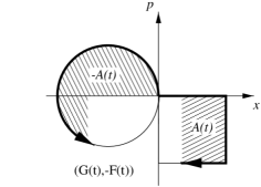
FIG. 2.: The paths traversed in phase space and the function $A(t)$ in Milburns proposal (rectangular) and in our proposal (circle).

Apart from a change of basis from $J_{z}$ to $J_{y}$ the interaction considered by Milburn[7] may also be put in this form, with $f(t)$ and $g(t)$ alternating between zero and non-vanishing constants. Within the present formulation, the trick in Ref.[7] is to use functions $f(t)$ and $g(t)$ such that $F(t)$ and $G(t)$ both vanish after a period $\tau$. At this instant the vibrational motion is returned to its original state and the propagator reduces to $U(\tau)={\rm e}^{-iA(\tau)J_{y}^{2}}$, i.e., we are left with an internal state evolution which is independent of the external vibrational state. This decoupling is possible because the effective internal state transition is completed in the same amount of time for all vibrational components and because the AC Stark shift of the atomic levels due to the laser fields are independent of the value of $n$. In the weak field case these properties are ensured by the interfering coupling amplitude in Fig. 1, see detailed discussion in Ref. [5]. In the general case it follow from the formal structure of Eq. (12). According to (13) the acquired factor $A(\tau)$ is equal to the area swept by the line segment between $(G(t),0)$ and $(G(t),-F(t))$, as shown in Fig. 2. If $(G(t),-F(t))$ forms a closed path, $A(t)$ is plus (minus) the enclosed area if the path is traversed in the (counter) clockwise direction. In the proposal by Milburn successive constant Hamiltonians proportional to $x$ and $p$ are applied and the area enclosed by $(G(t),-F(t))$ is rectangular. In our proposal the area is a circle of radius $\sqrt{2}J_{y}\eta\Omega/(\nu-\delta)$, as illustrated in Fig. 2.

With the propagator in Eq. (12) we may calculate the time evolution of the system. Suppose that the ions are initially in the internal ground state and an incoherent mixture of vibrational state as described by the density matrix $\rho^{tot}=\sum_{n}P_{n}|g..gn\rangle\langle g..gn|$. The time evolution of the internal state density operator $\rho={\rm Tr}_{n}(\rho^{tot})$ with any number of ions $N$ may be found from $\rho_{a_{1}...a_{N},b_{1}..b_{N}}(t)=\sum_{n}P_{n}\langle g..gn|U^{\dagger}(t)|b_{1}..b_{N}\rangle\langle a_{1}..a_{N}|U(t)|g..gn\rangle$ ($a_{j},b_{j}=e$ or $g$), where we have used $\sum_{n}|n\rangle\langle n|=1$ to remove one of the summations over vibrational states. Here we list the density matrix elements for the case of two ions $N=2$:

$$\rho_{gg,gg} = \sum_{n}P_{n}{\text{[}}\frac{3}{8}+\frac{1}{2}{\rm e}^{-\frac{F(t)^{2}+G(t)^{2}}{4}}$$ (21)

$$\times L_{n}{\left(\frac{F(t)^{2}+G(t)^{2}}{2}\right)}\cos{\left(A(t)+\frac{1}{2}F(t)G(t)\right)}$$

$$+\frac{1}{8}{\rm e}^{-(F(t)^{2}+G(t)^{2})}L_{n}{\left(2(F(t)^{2}+G(t)^{2})\right)}{\text{]}}$$

$$\rho_{ee,ee} = \sum_{n}P_{n}{\text{[}}\frac{3}{8}-\frac{1}{2}{\rm e}^{-\frac{F(t)^{2}+G(t)^{2}}{4}}$$ (24)

$$\times L_{n}{\left(\frac{F(t)^{2}+G(t)^{2}}{2}\right)}\cos{\left(A(t)+\frac{1}{2}F(t)G(t)\right)}$$

$$+\frac{1}{8}{\rm e}^{-(F(t)^{2}+G(t)^{2})}L_{n}(2(F(t)^{2}+G(t)^{2})){\text{]}}$$

$$\rho_{gg,ee} = \sum_{n}P_{n}{\text{[}}\frac{1}{8}(1-{\rm e}^{-(F(t)^{2}+G(t)^{2})}$$ (28)

$$\qquad\times L_{n}(2(F(t)^{2}+G(t)^{2})))$$

$$-\frac{i}{2}{\rm e}^{-\frac{F(t)^{2}+G(t)^{2}}{4}}L_{n}{\left(\frac{F(t)^{2}+G(t)^{2}}{2}\right)}$$

$$\qquad\times\sin{\left(A(t)+\frac{1}{2}F(t)G(t)\right)}{\text{]}},$$

where $L_{n}$ is the $n$’th order Laguerre polynomium.

These expressions can be evaluated in different regimes. In the weak field regime, $\eta\Omega<<\nu-\delta$, the $xp$ phase space trajectory is a very small circle, which is traversed several times. $F(t)$ and $G(t)$ are negligible for all times, and ${\rm e}^{-iF(t)J_{y}x}{\rm e}^{-iG(t)J_{y}p}$ is approximately unity, such that we have an internal state preparation which is disentangled from the vibrational motion throughout the gate. Since $A(t)\approx-\eta^{2}\Omega^{2}t/(\nu-\delta)$ if $(\nu-\delta)t>>1$ the time evolution corresponds to the one obtained from an effective Hamiltonian $H=\tilde{\Omega}J_{y}^{2}$, and Eq. (21) describes simple Rabi oscillations between the states $|gg\rangle$ and $|ee\rangle$. This is demonstrated in Fig. 3 (a) which shows the time evolution described by Eq. (21). The curves show sinusoidal Rabi oscillation from $|gg\rangle$ to $|ee\rangle$ superimposed by small oscillations due to the weak entanglement with the vibrational motion.

FIG. 3.: Time evolution of density matrix elements for two ions calculated from Eq (21). (a) Weak field regime (b) Fast gate. The first curve (counting from above at $\nu t\approx 1000$ in (a) and $\nu t\approx 130$ in (b)) represents $\rho_{gg,gg}$, the second is the imaginary part of $\rho_{gg,ee}$, the third is $\rho_{ee,ee}$, and the last curve is the real part of $\rho_{gg,ee}$. The ions are initially in the internal state $|gg\rangle$ and a thermal vibrational state with an average of 2 vibrational quanta. In (a) the physical parameters are $\delta=0.9\nu$, $\eta=0.1$, and $\Omega=0.1\nu$. In (b) the physical parameters are $\delta=0.95\nu$, $\eta=0.1$, and $\Omega=0.177\nu$. The parameters in (b) are chosen such that a maximally entangled state $\frac{1}{\sqrt{2}}(|gg\rangle-i|ee\rangle)$ is formed at the time $\nu t\approx 250$, where the circular path in Fig. 2 has been traversed twice.

Outside the weak field regime the internal state is strongly entangled with the vibrational motion in the course of the gate. For successful gate operation we have to ensure that we return to the initial vibrational state at the end of the gate by choosing parameters such that $G(\tau)=F(\tau)=0$, corresponding to $(\nu-\delta)\tau=K2\pi$, where $K$ is an integer. A maximally entangled state is created if we adjust our parameters so that $A(\tau)=-\pi/2$. This is achieved if the parameters are chosen in accordance with

$${\eta\Omega\over\nu-\delta}={1\over 2\sqrt{K}},\quad K=1,2,3,...\ .$$ (29)

By choosing a low value of $K$ such that an entangled state is created after a few rounds in phase space we may perform a faster gate than considered in the weak field case. See Fig. 3 (b), where we have used $K=2$, and where a maximally entangled state $\frac{1}{\sqrt{2}}(|gg\rangle-i|ee\rangle)$ is created at the time $\nu t\approx 250$.

By combining the requirement $(\ref{krav})$ with the condition $(\nu-\delta)\tau=K2\pi$ we may express the time for the state preparation as

$$\tau=\frac{\pi}{\eta\Omega}\sqrt{K}.$$ (30)

In order to avoid off-resonant excitations of the ions we must require $\frac{\Omega^{2}}{\nu^{2}}<<1$ and $\eta^{2}$ must be much less than unity to fulfill the Lamb-Dicke approximation (see subsec. III A and III B). For a given trap and/or laser intensity Eq. (30) sets a bound on the speed of the gate. In tabel I we give some numerical examples for the time of the gate for some typical experimental parameters. The control-not operation which plays a central role in quantum computation [1] may be created by a combination of single particle rotations and a bichromatic pulse with the duration described by Eq. (30). The single particle operations may be performed much faster than the two qubit gates, so the time required to perform a control-not operation is also given by (30).

TABLE I.: The time required to create the maximally entangled state $\frac{1}{\sqrt{2}}(|gg...g\rangle-i|ee..e\rangle)$ with a Lamb-Dicke parameter $\eta=0.1$ for various trapping frequencies ($\nu$) and laser intensities ($\Omega$). The table shows the gate time if the entangled state is prepared after a single round in phase space. If the gate operation is accomplished after $K$ rounds in phase space the time should be multiplied by $\sqrt{K}$.

$\frac{\Omega}{\nu}$	$\frac{\nu}{2\pi}=$500 KHz	1 MHz	10 MHz
0.05	200 $\mu$s	100$\mu$s	10 $\mu$s
0.10	100 $\mu$s	50 $\mu$s	5 $\mu$s
0.20	50 $\mu$s	25 $\mu$s	2.5 $\mu$s

III Non ideal conditions

In the previous section we used the Lamb-Dicke and the rotating wave approximations to arrive at an exactly solvable model. In this section we perform a more detailed analysis of the validity of the approximations and we estimate the effect of deviations from the ideal situation in an actual experiment. The general procedure in the section, is to change to the interaction picture with respect to the simple Hamiltonian (11) using the exact propagator in Eq. (12), and to treat the small deviations from the ideal situation by perturbation theory. The figure of merit for the performance of the gate is taken to be the fidelity $F$ of creation of the maximally entangled $N$-particle state $|\Psi_{max}\rangle=1/\sqrt{2}(|gg..g\rangle-i|ee..e\rangle)$, which in the ideal case is created at the time when $A(\tau)=-\pi/2$, if the ions are initially in the $|gg..g\rangle$ state [6], i. e.,

$$F=\langle\Psi_{max}|\rho_{int}(\tau)|\Psi_{max}\rangle.$$ (31)

A Direct coupling

Going from Eq. (10) to Eq. (11) we neglected a term $H_{d}=2\Omega J_{x}\cos(\delta t)$. This term describes direct off resonant coupling of $g$ and $e$ without changes in the vibrational motion. For high laser power this term has a detrimental effect on the fidelity, which we calculate below.

Changing to the interaction picture, we may find the propagator $U_{I}(t)$ from the Dyson series

$$U_{I}(t) = 1-i\int_{0}^{t}dt^{\prime}H_{d,I}(t^{\prime})$$ (33)

$$\quad-\int_{0}^{t}\int_{0}^{t^{\prime}}dt^{\prime}dt^{\prime\prime}H_{d,I}(t^{\prime})H_{d,I}(t^{\prime\prime})+\dots~{},$$

where the interaction Hamiltonian is given by $H_{d,I}(t)=U^{\dagger}(t)H_{d}(t)U(t)$. Since $H_{d}(t)$ is oscillating at a much higher frequency than the propagator $U(t)$, we may treat $U(t)$ as a constant during the integration and we obtain

$$U_{I}(t) = 1-i\frac{2\Omega}{\delta}\sin(\delta t)U^{\dagger}(t)J_{x}U(t)$$ (35)

$$\quad-\frac{\Omega^{2}}{\delta^{2}}(1-\cos(2\delta t))U^{\dagger}(t)J_{x}^{2}U(t)+\dots~{}.$$

Near the endpoint, $U(t)\approx{\rm e}^{i(\pi/2)J_{y}^{2}}$ and we obtain the fidelity

$$F\approx 1-\frac{N\Omega^{2}}{2\delta^{2}}(1-\cos(2\delta\tau)),$$ (36)

where $N$ is the number of ions participating in the gate. We plot in Fig. 4 the product of the fidelity due to the carrier (36) and the population of the EPR-state $\frac{1}{\sqrt{2}}(|gg\rangle-i|ee\rangle)$ expected from the time evolution in Eq. (21). The result agrees well with the result of a numerical integration of the Schrödinger equation with the Hamiltonian (10).

FIG. 4.: Population of the EPR-state $\frac{1}{\sqrt{2}}(|gg\rangle-i|ee\rangle)$ near the optimum. The full line is obtained by a numerical integration of the Hamiltonian (10) and the dashed line is the product of the expression in (36) and the expression for the fidelity obtained from Eq. (21). The parameters are the same as in Fig. 3 (b).

If the duration of the laser pulses can be controlled very accurately in the experiment, so that one fulfills both (29) and $2\delta\tau=2K^{\prime}\pi$ the effect of the direct coupling vanishes. If one cannot perform such an accurate control, the net effect of the direct coupling is to reduce the average fidelity by $\frac{N\Omega^{2}}{2\delta^{2}}$ (=0.03 for the parameters of Fig. 4).

B Lamb-Dicke approximation

In section II we used the Lamb-Dicke approximation ${\rm e}^{i\eta(a+a^{\dagger})}\approx 1+i\eta(a+a^{\dagger})$ to simplify our calculations. Now we investigate the validity of this approximation.

In the weak field case, we can use the exact matrix elements $\langle n|{\rm e}^{i\eta(a+a^{\dagger})}|n+1\rangle=i\eta\frac{{\rm e}^{-\eta^{2}/2}}{\sqrt{n+1}}L^{1}_{n}(\eta^{2})$, to obtain the effective Rabi frequency between $|ggn\rangle$ and $|een\rangle$

$$\tilde{\Omega}_{n} = \tilde{\Omega}{\rm e}^{-\eta^{2}}{\left[{{\left(L_{n}^{1}(\eta^{2})\right)^{2}}\over{n+1}}-{{\left(L_{n-1}^{1}(\eta^{2})\right)^{2}}\over{n}}\right]}$$ (37)

$$\approx \tilde{\Omega}{\left[1-\eta^{2}(2n+1)+\eta^{4}{\left(\frac{5}{4}n^{2}+\frac{5}{4}n+\frac{1}{2}\right)}\right]},$$ (38)

where $\tilde{\Omega}$ is given by Eq. (7), and where $L_{n}^{1}$ are the generalized Laguerre polynomials

$$L_{n}^{\alpha}(x)=\sum_{m=0}^{n}(-1)^{m}{\left(\begin{array}[]{cc}{n+\alpha}\\ {n-m}\end{array}\right)}\frac{x^{m}}{m!}.$$ (39)

The effective Rabi frequency is no longer independent of the vibrational quantum number $n$, and the internal state becomes entangled with the vibrational motion, resulting in a non-ideal performance of the gate [9].

To illustrate the effect of deviations from the Lamb-Dicke approximation, we consider again the production of an EPR-state $\frac{1}{\sqrt{2}}(|gg\rangle-i|ee\rangle)$. With an $n$-dependent coupling strength the fidelity is

$$F=\frac{1}{2}+\frac{1}{2}\sum_{n=0}^{\infty}P_{n}\sin(\tilde{\Omega}_{n}t),$$ (40)

where $P_{n}$ is the initial population of the vibrational state $n$. We show in Fig. 5 the evolution of the fidelity predicted by Eq. (40) and obtained by a direct integration of the full Hamiltonian in Eq. (6). Due to the deviation from the Lamb-Dicke approximation the effective Rabi frequency is reduced, cf., Eq. (37), and the optimal gate performance is achieved with a duration that is longer than $\pi/(2\tilde{\Omega})$. The spreading of the values of $\tilde{\Omega}_{n}$, causes entanglement with the vibrational motion which reduces the fidelity. With the parameters in Fig. 5 the maximally obtainable fidelity is 0.92 obtained after a pulse of duration $\tau\approx 1.9/\tilde{\Omega}$.

FIG. 5.: Evolution of the population of the EPR-state $\frac{1}{\sqrt{2}}(|gg\rangle-i|ee\rangle)$ for a vibrational thermal state with an average of 5 vibrational quanta and $\eta=0.20$. The dotted line is the prediction from Eq. (40) and the solid line is the result of a numerical integration of the Hamiltonian (6) with parameters $\Omega=0.02\nu$ and $\delta=0.9\nu$. The discrepancy between the two curves at $\tilde{\Omega}t\gtrsim 2$ is due to additional off-resonant couplings which may be taken into account by multiplying the coupling strength by $\frac{2\nu}{\nu+\delta}$ (dashed curve) [5, 6].

With more than two ions, the time evolution of the system may be obtained by expanding the initial state $|gg...g\rangle$ on eigenstates of the $J_{y}$ operator:

$$|gg...g\rangle=\frac{(-i)^{N}}{2^{N/2}}\sum_{k=0}^{N}(-1)^{k}\sqrt{{\left(\begin{array}[]{cc}{N}\\ {k}\end{array}\right)}}|M_{y}=N/2-k\rangle.$$ (43)

In the $J_{y}$ basis the propagator (12) is diagonal and in the weak field regime ($F(t)$, $G(t)\approx 0$) with $n$ dependent coupling strengths we get the fidelity

$$F={\sum_{n=0}^{\infty}}P_{n}{\left|\frac{1}{2^{N}}\sum_{k=0}^{N}{\left(\begin{array}[]{cc}{N}\\ {k}\end{array}\right)}{\rm e}^{i(N/2-k)^{2}(\pi/2-\tilde{\Omega}_{n}t)}\right|}^{2}.$$ (44)

In the limit of many ions $(N>>1)$ and near the optimum ($\tilde{\Omega}_{n}t\approx\pi/2$) we may approximate this expression by assuming that $k$ is a continuous variable and by replacing the binominal coefficient by a Gaussian distribution with the same width. In this limit the fidelity becomes

$$F=\sum_{n=0}^{\infty}P_{n}{{1}\over{\sqrt{1+\frac{N(N-1)(\pi/2-\tilde{\Omega}_{n}t)^{2}}{4}}}}.$$ (45)

Expanding this expression to lowest order in $\eta$ and adjusting the pulse duration to take into account the reduction in the coupling strength we find to lowest order in $\eta$

$$F=1-\frac{\pi^{2}N(N-1)}{8}\eta^{4}{\rm Var}(n)$$ (46)

at the optimum time

$$\tau_{opt}={\pi\over 2\tilde{\Omega}}(1+\eta^{2}(2\bar{n}+1)),$$ (47)

where $\bar{n}$ and Var$(n)$ are the mean and variance of the vibrational quantum number.

In Eq. (45) and (46) we have replaced a quantity $N^{2}$ following from the Gaussian approximation to (44) by $N(N-1)$. With this substitution (45) and (46) describe the fidelity well for all values of $N$. With the parameters of Fig. 5, Eq. (46) yields $F=0.88$ which is in good agreement with the numerical result in the figure.

The equations (37-46) were derived for weak fields, but they also provide an accurate description of the system outside this regime. To show this we note, that with bichromatic light, $H_{\rm int}$ in Eq. (6) may be written as

$$H_{\rm int} = 2\Omega\cos(\delta t){\Big{[}}J_{x}\cos{\left(\eta\sqrt{2}(x\cos(\nu t)+p\sin(\nu t))\right)}$$ (49)

$$\quad-J_{y}\sin{\left(\eta\sqrt{2}(x\cos(\nu t)+p\sin(\nu t))\right)}{\Big{]}}$$

in the interaction picture with respect to $H_{0}$. An expansion of the trigonometric functions in this Hamiltonian leads to Eq. (10) which formed the basis of the discussion in section II. The term proportional to $J_{x}$ is suppressed because it is far off resonance. The lowest order contribution of this term was treated in the previous section, and we shall now consider corrections to the $J_{y}$ term which may have significant effects. In the interaction picture with respect to the lowest order Hamiltonian (11), $x$ and $p$ are changed into $x+J_{y}G(t)$ and $p-J_{y}F(t)$ and to lowest non-vanishing order in $\eta$ the interaction picture Hamiltonian is

$$H_{3} = \eta^{3}J_{y}\frac{\sqrt{2}\Omega}{12}\Big{[}\cos((\nu-\delta)t)h_{1}(x,p)$$ (51)

$$\qquad\qquad\qquad+\sin((\nu-\delta)t)h_{2}(x,p)\Big{]},$$

where

$$h_{1}(x,p) = 3x^{3}+xp^{2}+pxp+p^{2}x$$ (52)

$$h_{2}(x,p) = 3p^{3}+px^{2}+xpx+x^{2}p,$$ (53)

and where we have used that $F(t)$ and $G(t)$ are proportional to $\eta$. To calculate the effect of the Hamiltonian in (51) we note that the propagator

$$U_{3,{\rm int}}(t)={\rm e}^{{\left[-i\frac{\sin((\nu-\delta)t)}{\nu-\delta}h_{1}(x,p)\right]}}{\rm e}^{{\left[-i\frac{1-\cos((\nu-\delta)t)}{\nu-\delta}h_{2}(x,p)\right]}}$$ (54)

is consistent with the Hamiltonian (51) until order $\eta^{5}$, i.e. $i\frac{dU_{3,{\rm int}}(t)}{dt}=(H_{3}+O(\eta^{6}))U_{3,{\rm int}}$. (But the full Hamiltonian contains terms of order $\eta^{4}$ and $\eta^{5}$ which are not taken into account in $U_{3,{\rm int}}$. These terms are included below). We are interested in the propagator at times $\tau=K2\pi/(\nu-\delta)$ where the vibrational motion is returned to the initial state. At these instants the exponents in Eq. (54) vanish and the propagator reduces to $U_{3}(\tau)=1$ such that it has no influence on the internal state preparation.

Expanding the Hamiltonian to order $\eta^{6}$ we obtain the propagator to the same order in $\eta$ in the interaction picture with respect to $H_{0}$ in (6)

$$U_{6}(\tau) = {\rm e}^{-i\tilde{\Omega}\tau J_{y}^{2}{\left[1-\eta^{2}(2n+1)+\eta^{4}{\left(\frac{5}{4}n^{2}+\frac{5}{4}n+\frac{1}{2}\right)}\right]}}$$ (56)

$$\quad\times{\rm e}^{i\eta^{5}J_{y}^{3}\frac{\sqrt{8}\Omega^{3}}{(\nu-\delta)^{2}}x\tau}{\rm e}^{-i\eta^{6}J_{y}^{4}\frac{5\Omega^{4}}{2(\nu-\delta)^{3}}\tau}$$

valid at times $\tau=K2\pi/(\nu-\delta)$. The first exponential provides the time evolution with the modified effective Rabi frequency in Eq. (37). If we evaluate the propagator (56) in the weak field regime, the last two exponentials both vanish in the limit of large K when the requirement (29) is inserted, and the time evolution in (56) is consistent with Eq. (37-46). The last two exponentials are also of minor importance for a different reason: In Eq. (37) $\eta^{2}$ appears in the combination $\eta^{2}n$, whereas it appears as $\eta^{2}$ in the last two exponentials of (56) when the condition (29) is inserted. In situations where deviations from the Lamb-Dicke approximation are important $\eta^{2}n\sim 1$, the deviation is typically caused by a high value of $n$ rather than a large value of $\eta$ ($\eta^{2}<<1$). In this case one may neglect the last two exponentials and the effect of the non-Lamb-Dicke terms are the same as in the case of weak fields as described by Eqs. (37-46). To achieve the optimum operation of the gate with the parameters of Fig. 5 we have to ensure $\tilde{\Omega}\tau\approx 1.9$ and there is a small correction to the condition in Eq. (29).

IV External disturbances

So far we have considered a system described by the Hamiltonian (6), where only the center of mass motion is present in the ion trap and where the coupling of this mode to the surroundings is neglible. In this section we shall remove these two assumptions and consider the decrease in fidelity due to the presence of other modes in the trap and due to heating of the center of mass vibrational motion.

A Spectator vibrational modes

With $N$ ions in the trap, the motional state is described by $3N$ non degenerate vibrational modes. With a proper laser geometry or if the transverse potential is much steeper than the longitudinal potential, the coupling of the laser to transverse modes will be neglible and the only contribution is from the $N$ longitudinal modes. With $N$ vibrational modes the ion trap may be described by the Hamiltonian

$$H= H_{0}+H_{{\rm int}}$$ (57)

$$H_{0}= \sum_{l=1}^{N}\nu_{l}(a_{l}^{\dagger}a_{l}+1/2)+\omega_{eg}\sum_{i}\sigma_{zi}/2$$ (58)

$$H_{{\rm int}}= \sum_{i=1}^{N}\frac{\Omega_{i}}{2}(\sigma_{+i}\ {\rm e}^{i(\sum_{l=1}^{N}\eta_{i,l}(a_{l}+a_{l}^{\dagger})-\omega t)}+h.c.),$$ (59)

where $\nu_{l}$ and $a_{l}^{\dagger}$ and $a_{l}$ are the frequency and ladder operators of the $l$’th mode. The excursion of the $i$’th ion in the $l^{\prime}th$ mode is described by the Lamb-Dicke parameter $\eta_{i,l}$ which may be represented as $\eta_{i,l}=\eta\frac{\sqrt{N}b_{i}^{l}}{\sqrt{\nu_{l}/\nu}}$, where $\eta$ and $\nu$ refer to the center of mass mode as in the previous sections, and where $b_{i}^{l}$ obeys the orthogonality conditions $\sum_{i=1}^{N}b_{i}^{l}b_{i}^{l^{\prime}}=\delta_{l,l^{\prime}}$ and $\sum_{l=1}^{N}b_{i}^{l}b_{i^{\prime}}^{l}=\delta_{i,i^{\prime}}$ [10].

The center of mass mode ($l=1$), which is used to create the entangled states of the ions, has $b_{i}^{1}=1/\sqrt{N}$ for all ions and is well isolated from the remaning $N-1$ vibrational modes $\nu_{l>1}\geq\sqrt{3}\nu$, so that we could neglect the contribution from the other modes in the previous sections. In this section we shall extimate the effect of the presence of the spectator modes. They have both a direct effect, due to the off resonant coupling to the other modes, and an indirect ’Debye-Waller’ effect [11] because the coupling strength of the center of mass mode is reduced due to the oscilations in the spectator modes. Below we shall calculate the direct and indirect effects separately.

The lowest order contribution of the direct coupling to the spectator modes may be found by expanding the exponentials as in Eq. (10).

$$H_{\rm int}= 2\Omega J_{x} \cos\delta t+\sum_{l=1}^{N}\Theta_{l}[x_{l}f_{l}(t)+p_{l}g_{l}(t)],$$ (60)

where $f_{l}(t)=-\sqrt{2}\eta\Omega\sqrt{\nu/\nu_{l}}[\cos(\nu_{l}-\delta)t+\cos(\nu_{l}+\delta)t]$ and $g_{l}(t)=-\sqrt{2}\eta\Omega\sqrt{\nu/\nu_{l}}[\sin(\nu_{l}-\delta)t+\sin(\nu_{l}+\delta)t]$, and where the internal and external state operators are defined by $\Theta_{l}=\sum_{i=0}^{N}b_{i}^{l}j_{y,i}$ and $x_{l}=\frac{1}{\sqrt{2}}(a_{l}+a_{l}^{\dagger})$ and $p_{l}=\frac{i}{\sqrt{2}}(a_{l}^{\dagger}-a_{l})$. Since the ladder operators for different modes commute, we may find the propagator for this Hamiltonian using the steps that lead to Eq. (12)

$$U(t)=\prod_{l=1}^{N}U_{l}(t),$$ (61)

where

$$U_{l}(t)={\rm e}^{-iA_{l}(t)\Theta_{l}^{2}}{\rm e}^{-iF_{l}(t)\Theta_{l}x_{l}}{\rm e}^{-iG_{l}(t)\Theta_{l}p_{l}}$$ (62)

with the functions $F_{l}$, $G_{l}$ and $A_{l}$ defined analogously to Eq. (13). Note, that this is an exact solution of the Hamiltonian (60) without the $J_{x}$ term, so that to lowest order in the Lamb-Dicke parameter it includes all effects of the coupling to the other modes.

From the definition of $\Theta_{l}$ it is seen that $\Theta_{1}=J_{y}$ and the propagator $U_{1}$ reduces to Eq. (12) in the rotating wave approximation. The other $N-1$ propagators in (61) cause a reduction of the fidelity due to the excursion into the $x_{l}p_{l}$ phase space of these modes. Expanding the exponentials, using $\langle gg...g|\Theta_{l}\Theta_{l^{\prime}}|gg...g\rangle=\delta_{l,l^{\prime}}N/4$ and $\delta\approx\nu$, and averaging over time we find

$$F=1-\eta^{2}N\frac{\Omega^{2}}{\nu^{2}}\sum_{l=2}^{N}\frac{\nu}{\nu_{l}}(2\bar{n}_{l}+1)\frac{\nu_{l}^{2}/\nu^{2}+1}{(\nu_{l}^{2}/\nu^{2}-1)^{2}},$$ (63)

where $\bar{n}_{l}$ is the mean vibrational excitation of the $l^{\prime}th$ mode.

In addition to the direct coupling to the spectator vibrational mode, the fidelity is also reduced because the coupling strength is dependent on the vibration of the other modes. Unlike the direct coupling discussed above, this effect is not suppressed by the other modes being far off-resonant, and it may have an effect comparable to the direct coupling.

Due to the vibration of the ions the coupling of the $i$’th ion to the sideband is reduced from $i\eta\sqrt{n+1}$ to $\langle n_{1}n_{2}...n_{N}|{\rm e}^{i\sum_{l=1}^{N}\eta_{i,l}(a_{l}+a_{l}^{\dagger})}|n_{1}+1n_{2}...n_{N}\rangle\approx i\eta\sqrt{n+1}(1-\sum_{l=1}^{N}\eta_{i,l}^{2}(n_{l}+1/2))$. With this reduced coupling strength the effective propagator at times $\tau=K2\pi/(\nu-\delta)$ may be described by

$$U(\tau)={\rm e}^{-iA(\tau)\Lambda^{2}},$$ (64)

where $\Lambda=\sum_{i=1}^{N}j_{y,i}(1-\sum_{l=1}^{N}\eta_{i,l}^{2}(n_{l}+1/2))$. In the Cirac-Zoller scheme [4], the $n$-dependent AC Stark shifts caused by coupling to other vibrational modes lead to decoherence, unless these modes are cooled to the ground state. In our bichromatic scheme, these internal state level shifts depend much less on the vibrational excitation. By expanding (64) around the optimum $A(t)\approx\pi/2$ we calculate the lowest order reduction in the fidelity

$$F = 1-\frac{\pi^{2}N(N-1)}{8}\eta^{4}\sum_{l=1}^{N}\frac{{\rm Var}(n_{l})}{(\nu_{l}/\nu)^{2}}$$ (66)

$$\quad-\frac{\pi^{2}(N-2)}{16}\eta^{4}\sum_{i,l,l^{\prime}=1}^{N}\frac{(b_{i}^{l})^{2}(b_{i}^{l^{\prime}})^{2}-1/N^{2}}{\nu_{l}\nu_{l^{\prime}}/\nu^{2}}\overline{n_{l}n_{l^{\prime}}}.$$

The expressions in Eqs. (63) and (66) may be simplified if the vibrational motion is in a thermal equilibrium at a given temperature. In a thermal state Var$(n_{l})=\bar{n}_{l}^{2}+\bar{n}_{l}$, $\overline{n_{l}n_{l^{\prime}}}=\bar{n}_{l}\bar{n}_{l^{\prime}}$ for $l\neq l^{\prime}$, and $\bar{n}_{l}\leq\bar{n}_{1}\nu/\nu_{l}$, and using these expressions we find the lower estimate for the fidelity

$$F\geq 1-\eta^{2}N\frac{\Omega^{2}}{\nu^{2}}(\bar{n}_{1}\sigma_{1}(N)+\sigma_{2}(N))$$ (67)

for the direct coupling (63) and

$$F \geq 1-\frac{\pi^{2}N(N-1)}{8}\eta^{4}(\bar{n}_{1}^{2}\sigma_{3}(N)+\bar{n}_{1}\sigma_{4}(N))$$ (69)

$$\quad-\frac{\pi^{2}(N-2)}{16}\eta^{4}(\bar{n}_{1}^{2}\sigma_{5}(N)+\bar{n}_{1}\sigma_{6}(N))$$

for the Debye-waller coupling (66), where the sums $\sigma_{1}...\sigma_{6}$ may be derived from Eqs. (63) and (66). For example $\sigma_{3}(N)=\sum_{l=1}^{N}\frac{\nu^{4}}{\nu_{l}^{4}}$. With the mode functions and frequencies of Ref. [10] these sums are readily evaluated, and the results are shown in Fig. 6. From the figure it is seen that $\sigma_{5},\sigma_{6}<<\sigma_{3},\sigma_{4}$, so that the last term in Eq. (69) may be neglected. All the sums have a very rapid convergence and we may estimate the fidelity by replacing the sums with their large $N$ values, i.e.

$$F\geq 1-\eta^{2}N\frac{\Omega^{2}}{\nu^{2}}0.8(\bar{n}_{1}+1)$$ (70)

for the direct coupling (63) and

$$F \geq 1-\frac{\pi^{2}N(N-1)}{8}\eta^{4}(1.2\bar{n}_{1}^{2}+1.4\bar{n}_{1})$$ (71)

for the Debye-Waller coupling (66).

We note that Eq. (71) is derived from terms beyond the Lamb-Dicke expansion and it incorporates the reduction of fidelity due to deviations from the Lamb-Dicke approximation in the center of mass mode, cf. the formal similarity of Eq. (71) and Eq. (46).

FIG. 6.: Evaluation of the sums $\sigma_{1}...\sigma_{6}$ for different number of ions $N$. Starting from above at $N\approx 5$ the curves represent $\sigma_{4}$, $\sigma_{3}$, $\sigma_{1}$, $\sigma_{2}$, $\sigma_{6}$, and $\sigma_{5}$.

B Heating of the vibrational motion

An ion trap cannot be perfectly isolated and the vibration of the ions will be subject to heating due to the interaction with the environment. Relaxation due to the interaction between the vibration and a thermal reservoir may be described by the master equation

$$\frac{d}{dt}\rho=-i{\left[H,\rho\right]}+{\cal L}(\rho),$$ (72)

where $\cal{L}(\rho)$ is of the Lindblad form

$${\cal L}(\rho)=-\frac{1}{2}\sum_{m}{\left(C_{m}^{\dagger}C_{m}\rho+\rho C_{m}^{\dagger}C_{m}\right)}+\sum_{m}C_{m}\rho C_{m}^{\dagger}$$ (73)

with relaxation operators $C_{1}=\sqrt{\Gamma(1+n_{th})}a$ and $C_{2}=\sqrt{\Gamma(n_{th})}a^{\dagger}$, where $\Gamma$ characaterizes the strength of the interaction, and $n_{th}$ is the mean vibrational number in thermal equilibrium.

We calculate the effect of heating assuming that the ions remain in the Lamb-Dicke limit. Changing to the interaction picture with respect to the Hamiltonian (11), the time evolution of $\rho$ is entirely due to the heating, i.e., the Lindblad terms which are transformed using the propagator (12)

$$\tilde{C_{1}} = U^{\dagger}C_{1}U=\sqrt{\Gamma(1+n_{th})}{\left(a+J_{y}\frac{G(t)-iF(t)}{\sqrt{2}}\right)}$$ (74)

$$\tilde{C_{2}} = U^{\dagger}C_{2}U=\sqrt{\Gamma n_{th}}{\left(a^{\dagger}+J_{y}\frac{G(t)+iF(t)}{\sqrt{2}}\right)}.$$ (75)

The density matrix is most conveniently expressed in the basis of $J_{y}$ eigenstates, and by tracing over the vibrational states we find the time derivative of the internal state density matrix in the interaction picture

$$\frac{d}{dt}\rho_{M_{y},M_{y}^{\prime}} = -(M_{y}-M_{y}^{\prime})^{2}\Gamma(1+2n_{th})$$ (77)

$$\quad\quad\times\frac{G(t)^{2}+F(t)^{2}}{4}\rho_{M_{y},M_{y}^{\prime}}.$$

This equation is readily integrated, and at times $\tau=K2\pi/(\nu-\delta)$ we get

$$\rho_{M_{y},M_{y}^{\prime}}(\tau)=\rho_{M_{y},M_{y}^{\prime}}(0){\rm e}^{-(M_{y}-M_{y}^{\prime})^{2}\frac{\Gamma(1+2n_{th})}{4K}\tau}.$$ (78)

The initial state is expanded on the $J_{y}$ eigenstates as in Eq. (43) and the population of the initial state (which is ideally constant in the interaction picture) equals

$$F=\frac{1}{2^{2N}}\sum_{j=0}^{N}\sum_{k=0}^{N}{\left(\begin{array}[]{cc}{N}\\ j\end{array}\right)}{\left(\begin{array}[]{cc}{N}\\ k\end{array}\right)}{\rm e}^{-(j-k)^{2}\frac{\Gamma(1+2n_{th})}{4K}\tau}.$$ (79)

For two ions this expressions can be readily evaluated

$$F=\frac{3}{8}+\frac{1}{2}{\rm e}^{-\frac{\Gamma(1+2n_{th})}{4K}\tau}+\frac{1}{8}{\rm e}^{-4\frac{\Gamma(1+2n_{th})}{4K}\tau}.$$ (80)

In the limit of many ions ($N>>1$) and short times ($\frac{\Gamma(1+2n_{th})}{4K}\tau<<1$) we may again approximate the expression in Eq. (79) by assuming that $j$ and $k$ are continuous variables and by replacing the binomial coefficients by Gaussian distributions with the same width. In this limit the fidelity becomes

$$F={{1}\over{\sqrt{1+N\frac{\Gamma(1+2n_{th})}{4K}\tau}}}.$$ (81)

For 2 ions the deviation between (80) and (81) is less than 0.02 for all values of $F$ larger than $0.5$.

In the above expressions we have assumed the Lamb-Dicke approximation. This corresponds to a situation where the heating is counteracted for example by lasercooling on some ions reserved for this purpose. If the ions are not cooled the heating will proceed towards high vibrational numbers with a heating rate $\Gamma n_{th}$ and the heating will eventually take the ions out of the Lamb-Dicke limit. With strong fields ($K\sim 1$) the reduction in the fidelity described by Eq. (81) will ruin the entangled state before the heating has made a significant change to the vibrational state ($\Gamma n_{th}\tau\gtrsim 1$). For weak fields ($K>>1$) however, the situation is different. With weak fields one may produce an entangled state even though the time required to entangle the ions is much longer than the decoherence time of the vibrational motion which is used to communicate between the ions, i.e. if $K>N\Gamma n_{th}\tau$ the effect of heating is small even though the change in the average vibrational number $\Gamma n_{th}\tau$ is larger than unity [5, 6]. Since the effective Rabi-frequency has a small dependence on the vibrational quantum number $n$ as described in Eq. (37) the heating will have an indirect effect on the internal state preparation. This can be modelled by changing the probabilities in Eqs. (40-45) into time dependent functions $P_{n}(t)$ reflecting the change in the vibrational motion occurring during the internal state preparation.

TABLE II.: Creation of entangled states of $N$ ions $\frac{1}{\sqrt{2}}(|gg...g\rangle-i|ee...e\rangle)$ by interaction with a bichromatic field (10) $H_{\rm int}=2\Omega J_{x}\cos\delta t-\sqrt{2}\eta\Omega J_{y}[x(\cos(\nu-\delta)t+\cos(\nu+\delta)t)+p(\sin(\nu-\delta)t+\sin(\nu+\delta)t)]$ obeying $\frac{\eta\Omega}{\nu-\delta}=\frac{1}{2\sqrt{K}}$, $K=1,2,3,...$ and for a duration $\tau=2\pi K/(\nu-\delta)$. The fidelity of the preparation is reduced by various causes, listed in the table.

Cause of deviation	Direct off-resonant coupling $J_{x}$ term in (10)	Deviations from Lamb-Dicke $\langle n|{\rm e}^{i\eta(a+a^{\dagger})}|n+1\rangle$          $\neq i\eta\sqrt{n+1}$	Spectator vibrational modes		Heating of the vibration towards vibrational number $n_{th}$ with rate $\Gamma n_{th}$
			(i) Direct coupling to other modes	(ii) Debye-Waller
$1-F$	${N\Omega^{2}\over 2\delta^{2}}$	$\eta^{4}{\pi^{2}N(N-1)\over 8}{\rm Var}(n_{1})$	$N{\eta^{2}\Omega^{2}\over\nu^{2}}0.8(\bar{n}_{1}+1)$	$\eta^{4}\frac{\pi^{2}N(N-1)}{8}$ $\times(0.2\bar{n}_{1}^{2}+0.4\bar{n}_{1})$	$N{\Gamma(1+2n_{th})\tau\over 8K}$
Eq.	(36)	(46)	(70)	(71) minus (46)	(81)

V Conclusion

We have in this paper evaluated the possibility for preparation of entangled states of ions by illumination with bichromatic light. We have identified two regimes: (i) a weak field regime where single photon absorption is suppressed and where two-photon processes interfere in a way that makes the internal state dynamics insensitive to the vibrational state, and (ii) a strong field regime where the individual ions are coherently excited and the motional state is highly entangled with the internal state until all undesirable excitations are deterministically removed towards the end of the interaction.

We have presented analytical estimates for the fidelity of the internal state preparation. These expressions are summarized in table II. The expressions for the fidelity may be readily applied to experimental parameters and they show that several ion trap experiments today are in a position to apply our proposal directly. In fact, using our proposal the NIST group at Boulder has been able to produce the maximally entangled state $\frac{1}{\sqrt{2}}(|gggg\rangle-i|eeee\rangle)$ with four ions [12]. In this experiment the heating of the center-of-mass mode was so strong that this mode could not be used to communicate between the ions. Instead the experiment used an asymmetric mode where all ions have the same amplitude but a different sign, i.e. $|\eta_{i}|$ are the same for all ions $i$. Apart from the center-of-mode such modes only exist in ion traps containing two or four ions, and the experiment could not go beyound four ions. In other existing traps the heating is much less significant [13], and these traps may be employed to produce entangled states with more particles.

The use of ancillary degrees of fredom (center-of-mass position and momentum) to communicate between two or more quantum systems is a key ingredient of quantum information processing. The algebraic property (3) which allows coupling and temporary entanglement with such an ancilla may find wide applications in many different systems for quantum computation with different ancillae (photons, phonons, Cooper-pairs, etc.). However, operators with a constant non-vanishing commutator (which allows the formal step from Eq. (2) to Eq. (3)) only exist in infinite-dimensional Hilbert spaces [14]. In addition to the implementation in cavity QED realizations of quantum computing [15, 16, 17] where quantized cavity fields play the role of the vibrational modes, it thus seems very relevant to investigate to which extent the ideas underlying Eq. (3) can be generalized to ancillae with a finite number of states and, e.g., for communication across a linear qubit register by only nearest neighbour interaction.

REFERENCES

- [1] A. Barenco, C. H. Bennet, R. Cleve, D. P. DiVincenzo, N. Margolus, P. Shor, T. Sleator, J. A. Smolin, and H. Weinfurter, Phys. Rev. A 52, 3457 (1995).
- [2] L. Viola, E. Knill, S. Lloyd, Phys. Rev. Lett. 82, 2417 (1999); P. Zanardi, Phys. Lett. A 258, 77 (1999).
- [3] S. Lloyd, Science 273, 1073 (1996).
- [4] J. I. Cirac and P. Zoller, Phys. Rev. Lett. 74, 4091 (1995).
- [5] A. Sørensen and K. Mølmer, Phys. Rev. Lett. 82, 1971 (1999).
- [6] K. Mølmer and A. Sørensen, Phys. Rev. Lett. 82, 1835 (1999).
- [7] G. Milburn, quant-ph/9908037.
- [8] J. J. Bollinger, W. M. Itano, D. J. Wineland, and D. J. Heinzen, Phys. Rev. A 54, 4649 (1996).
- [9] In Phys. Rev. A 59 R2539 (1999), E. Solano, R. L. de Matos Filho, and N. Zagury show how this -dependent coupling may be used to map out the ionic vibrational Wignerfunction. See also R. L. de Matos Filho and W. Vogel Phys. Rev. Lett. 76 4520 (1996).
- [10] D. F. V. James, Appl. Phys. B 66, 181 (1998).
- [11] D. J. Wineland, C. Monroe, W. M. Itano, D. Leibfried, B. E. King, and D. M. Meekhof, J. Res. Natl. Inst. Stand. Tech. 103, 259 (1998).
- [12] C. A. Sackett, D. Kielpinski, B. E. King, C. Langer, V. Meyer, C. J. Myatt, M. Rowe, Q. A. Turchette, W. M. Itano, D. J. Wineland, and C. Monroe, Nature 404, 256 (2000).
- [13] Ch. Roos, Th. Zeiger, H. Rohde, H. C. N gerl, J. Eschner, D. Leibfried, F. Schmidt-Kaler, and R. Blatt, Phys. Rev. Lett. 83, 4713 (1999).
- [14] If operators and have a constant commutator , then . If is finite, the left hand side vanishes due to the cyclic property of the trace and thus .
- [15] P. Domokos, J. M. Raimond, M. Brune, and S. Haroche, Phys. Rev. A 52 3554 (1995).
- [16] Q. A. Turchette, C. J. Hood, W. Lange, H. Mabuchi, and H. J. Kimble, Phys. Rev. Lett. 75 4710 (1995).
- [17] M. S. Sherwin, A. Imamolu, and T. Montroy, Phys. Rev. A 60 3508 (1999); A. Imamolu, D. D. Awschalom, G. Burkard, D. P. DiVincenzo, D. Loss, M. Sherwin, and A. Small, Phys. Rev. Lett. 83 4204.