Tailoring of vibrational state populations with light-induced potentials in molecules

Abstract

We propose a method for achieving highly efficient transfer between the vibrational states in a diatomic molecule. The process is mediated by strong laser pulses and can be understood in terms of light-induced potentials. In addition to describing a specific molecular system, our results show how, in general, one can manipulate the populations of the different quantum states in double well systems.

Quantum control of molecular processes has recently opened new possibilities for controlling chemical processes, and also for understanding the multistate quantum dynamics of molecular systems. With strong and short laser pulses one can create quantum superpositions of vibrational and continuum states, i.e., wave packets, which often propagate like classical objects under the influence of molecular electronic potentials [2]. Typically in spectroscopy one induces with laser light population transfer between individual vibrational states, and describes the process using Franck-Condon factors, perturbation theory and a very truncated Hilbert space for the molecular wave functions. If the laser light comes in as a very short pulse we expect to couple many vibrational states because of the broad spectrum. However, in this Letter we show that it is possible to start from a single vibrational state, and end up selectively on another single vibrational state, with very high efficiency, even when one uses strong and fast laser pulses.

We have previously discussed how one can transfer the vibrational ground state population of one electronic state to the vibrational ground state of another electronic state [3]. This process was called adiabatic passage in light-induced potentials (APLIP). These potentials, which depend on time, due to the time dependence of the laser pulse envelopes, provide a useful description of the process (see e.g. Ref. [4] and references therein). Here we use the same kind of light-induced potentials to describe and understand transfer processes between excited vibrational states. However, we will see that the process is more complicated than the simple adiabatic following assumed in APLIP.

FIG. 1.: (a) The three Na₂ potential energy surfaces used in our calculations: X${}^{1}\Sigma_{g}^{+}$, A${}^{1}\Sigma_{u}^{+}$ and 2${}^{1}\Pi_{g}$. (b) The shifted potentials. Here we have set $\Delta=\Delta_{1}=-\Delta_{2}$, [see Eq. (2)] and show the position of the intermediate A${}^{1}\Sigma_{u}^{+}$ state (dotted line) in respect to the other two electronic states (solid lines) for $\hbar\Delta=\pm 2000$ cm^-1.

To demonstrate the new process we have chosen the same Na dimer potentials, shown in Fig. 1(a), as in our previous study [3]. The three electronic states are coupled in a ladder formation by two laser pulses. Instead of describing the system in terms of the vibrational states and Franck-Condon factors, we consider only the electronic state wave functions, $\Psi_{i}(R,t)$, $i=X,A,\Pi$. If we apply the rotating wave approximation, we can ‘shift’ the $X^{1}\Sigma_{g}^{+}$ and $2^{1}\Pi_{g}$ state potentials in energy by the corresponding laser photons. Then we obtain the situation shown in Fig. 1(b), after a suitable redefinition of the energy zero point. The resonances between the electronic state potentials now become curve crossings. The evolution of the three wave functions $\Psi_{i}(R,t)$ is given by the time-dependent Schrödinger equation with the Hamiltonian

$$H=-\frac{\hbar^{2}}{2m}\frac{\partial^{2}}{\partial R^{2}}\ {\cal I}+{\cal U}(R,t)$$ (1)

where $R$ is the internuclear separation, $m$ is the reduced mass of the molecule, and the electronic potentials and couplings are given by

$${\cal U}(R,t)=\left[\begin{array}[]{ccc}U_{X}(R)&\hbar\Omega_{1}(t)&0\\ \hbar\Omega_{1}(t)&U_{A}(R)+\hbar\Delta_{1}&\hbar\Omega_{2}(t)\\ 0&\hbar\Omega_{2}(t)&U_{\Pi}(R)+\hbar(\Delta_{1}+\Delta_{2})\end{array}\right].$$ (2)

Here $U_{X}(R)$, $U_{A}(R)$, and $U_{\Pi}(R)$ are the three potentials, $\Delta_{1}$ and $\Delta_{2}$ are the detunings of the two pulses from the lowest points of the potentials [dashed lines in Fig. 1(a)], and $\Omega_{1}(t)=\mu_{XA}E_{1}(t)/\hbar$, $\Omega_{2}(t)=\mu_{A\Pi}E_{2}(t)/\hbar$ are the two Rabi frequencies. We have assumed for simplicity that the two dipole moments are independent of $R$ and we have used Gaussian pulse shapes, $\Omega_{i}(t)=\Omega\exp\{-[(t-t_{i})/T]^{2}\}$, $i=1,2$.

The light-induced potentials are obtained by diagonalising the potential term (2). For these potentials the curve crossings become avoided crossings. It is easy to see from Fig. 1(b) that in the absence of the pulses (or when they both are weak) one of the light-induced states corresponds, at low energies, to the double well structure formed by the $X^{1}\Sigma_{g}^{+}$ and $2^{1}\Pi_{g}$ electronic state potentials. In Fig. 1(b) this corresponds to the lower part of the two solid curves and we will call this the active eigenstate. In Ref. [3] we showed that, if the pulses are applied in a counterintuitive order ($t_{1}>t_{2}$), the double well structure will disappear as the bottom of the (initially empty) well on the right moves up and vanishes. (In Fig. 1(b) this is seen to be because of a repulsion between the $2^{1}\Pi_{g}$ and A${}^{1}\Sigma_{u}^{+}$ ($\Delta<0$) state). After this the left well broadens and moves to the right. Finally the double well structure is re-established as the pulses reduce in intensity. If we now consider that the ground vibrational state of the left well is initially populated, that population would follow the light-induced potential and be transformed smoothly into the ground state wave function of the right well. This is APLIP, and the smooth change in the total wave function is demonstrated in the contour plot in Fig. 2(a).

If we choose $\Delta_{1}=-\Delta_{2}\equiv\Delta$, the bottoms of the two wells are on the same level initially and finally [as in Fig. 1(b)]. The sign of $\Delta$ determines the evolution of the light-induced potential. For negative $\Delta$ we obtain the APLIP situation, but for positive $\Delta$ the right well drops down at first, instead of disappearing. In this case the APLIP situation is not obtained.

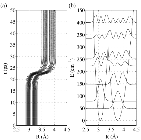
FIG. 2.: (a) The APLIP process for $\hbar\Delta=-3000$ cm^-1, $\hbar\Omega=2000$ cm^-1, $t_{1}=25.5$ ps, $t_{2}=20.5$ ps, and $T=5.5$ ps. (b) The active light-induced state (independent of $\Delta$ at low energies) when the pulses are absent ($\Omega=0$). We also show the seven lowest vibrational eigenstates $|\phi_{i}(R)|^{2}$ of the potential. The left well corresponds to X${}^{1}\Sigma_{g}^{+}$ and the right one to 2${}^{1}\Pi_{g}$.

One is tempted to associate the APLIP process with STIRAP [5], and consider the active light-induced potential as a dark state [6], which, because of the counterintuitive pulse order, remains uncoupled from the other states. It is true that during the APLIP process the intermediate state ($A^{1}\Sigma_{u}^{+}$) population remains very small. However, the process is not the same as STIRAP, because the strength of the atom-light coupling, i.e. Rabi frequency, becomes much larger than the vibrational spacing; it is not possible to isolate only a few energy levels. Furthermore, in a STIRAP process there would not be a smooth transport of the wave packet in Fig. 2(a) because only two simple vibrational eigenfunctions would be involved.

STIRAP is also considered to be an adiabatic process, which is not strictly the case for Fig. 2. We can see this by considering the initial (and final) vibrational states of the active light-induced potential which matches the two original electronic potentials as shown in Fig. 2(b). The lowest states correspond to the individual vibrational states of the original potentials. In STIRAP we should start with the lowest state on left, and we would expect it to evolve adiabatically into the lowest state on the right, though not in the smooth way seen for the APLIP process in Fig. 2(a). However, if the evolution were truly adiabatic the population would remain in the left well; by definition of adiabatic following it cannot change state. This is because, for the example shown in Fig. 2(b), as the right well rises up, and the right-hand-well wave function with it, there is a diabatic crossing of the energy states which allows the population to remain in the left well as the right well vanishes. As long as the barrier between the two wells is thick enough, the crossing of vibrational eigenenergies remains diabatic (uncoupled) and the wave packet (left-hand well vibrational ground state) can be channelled from left to right (APLIP). There always has to be at least one such diabatic crossing, but if there is only one, it could come at the start, or the end, of the time evolution depending on whether the initial or final vibrational state is lower in energy. Thus the interesting processes mediated by the light-induced potentials are different from STIRAP, and they can not be obtained by perfect adiabatic following.

Figure 2(b) also displays the initial and final situation if we now switch to a positive detuning. We choose $\hbar\Delta=2010$ cm^-1 for the time evolution shown in Fig. 3(a) where $\hbar\Omega=733$ cm^-1 and $t_{1}-t_{2}=T=5.5$ ps. We denote the vibrational quantum number of the states in the electronic potential with $\nu$, and indicate with the terms “left well” and “right well”, whether these states correspond to the initial state ($X^{1}\Sigma_{u}^{+}$), or the final state ($2^{1}\Pi_{g}$), respectively. We transfer the $\nu=0$ state on the left well into the $\nu=1$ state on the right well. The process is very efficient: the occupation probability of the right well ($2^{1}\Pi_{g}$ state) in the end is 94 %. Clearly the crucial moment is around $t=20$ ps where the original single-peak distribution extends to the right and forms temporarily a four-peaked distribution over the combined well system. Also, around $t=25$ ps the four-peak structure compresses into the two-peak structure located on the right well.

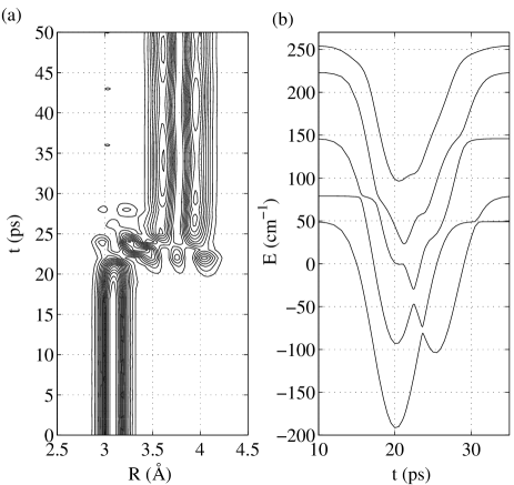
FIG. 3.: (a) The vibrational state tailoring with $\hbar\Delta=2010$ cm^-1, $\hbar\Omega=733$ cm^-1, $t_{1}=25.5$ ps, $t_{2}=20.5$ ps, and $T=5.5$ ps. Here we show the time evolution of the total probability distribution $|\Psi(R,t)|^{2}=\sum_{i}|\Psi_{i}(R,t)|^{2}$. (b) The time-dependent eigenenergies of the five lowest vibrational states of the active light-induced potential for the situation shown in (a). [Note that for $t\lesssim 15$ ps and $t\gtrsim 35$ ps the eigenstates match those seen in Fig. 2(b).]

In order to understand the process, we have calculated the time dependence of the eigenenergies of the active light-induced potential [seen for initial and final time in Fig. 2(b)]. The figure shows clearly that if the evolution is fully adiabatic, no change of $\nu$ can occur during the time evolution because there are no crossings of eigenenergies. This also means that no change of well is possible either. However, we do see several avoided crossings between the eigenenergies and the point is that when the pulses are weak, these crossings are passed diabatically, and when the pulses are strong they are passed adiabatically.

In our example, Fig. 3(b), the second lowest state corresponds initially, and finally, to the lowest vibrational state of the left well (i.e., the state populated initially in our calculation) as may be confirmed by inspecting Fig. 2(b). During the time evolution the wave function passes the two first avoided crossings diabatically, but for $t>20$ ps it follows nearly adiabatically the fourth eigenstate. Just before $t=30$ ps it moves diabatically onto the third eigenstate, which asymptotically corresponds with the $\nu=1$ state on the right well [see again Fig. 2(b)]. In Fig. 4 we show the change at the crucial moment around $t=21$ ps. The transition from a narrow single well wave function into a wide combined two-well wave function takes place very quickly. A fascinating aspect is that the evolution of the total wave function still follows the fourth vibrational eigenstate of the active light-induced potential. A similar adiabatic following happens also near $t=25$ ps when the third and the fourth eigenstate again approach each other.

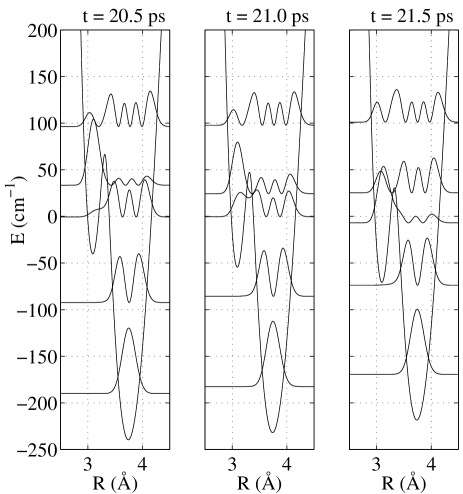
FIG. 4.: The behaviour of the eigenstates of the active light-induced potential in the situation of Fig. 3. We see how the fourth eigenstate deforms within 1 ps from the initial single-peak structure into the four-peak one. An inverse process happens to the third eigenstate. In the diabatic situation the system would follow the single-well eigenstates, thus jumping from the fourth state to the third. However, here the system instead follows the fourth state nearly adiabatically.

The example given here is not unique. By allowing $\Delta_{1}\neq-\Delta_{2}$ we have a very good handle in choosing which single well states are paired into a combined well state. In Fig. 5 we show two other examples. They demonstrate that the process does not require the initial state on the left to be $\nu=0$, and the process can be used also to change $\nu$ but keep the initial and final well the same [7].

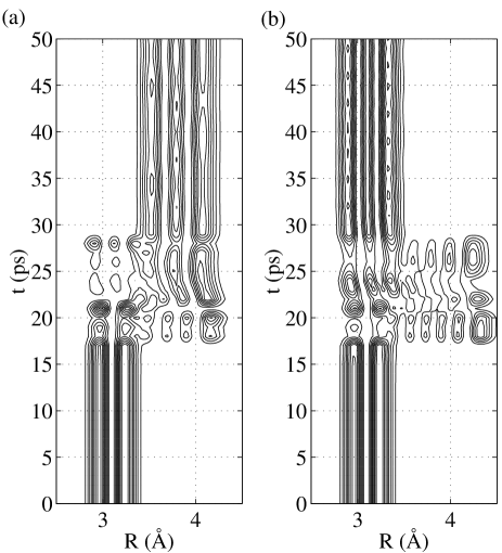
FIG. 5.: The state tailoring process with $\nu=1$ in the left well as the initial state. (a) $\nu=2$ in the right well as the final state. Here $\hbar\Delta_{1}=2010$ cm^-1 and $\hbar\Delta_{2}=-1960$ cm^-1. (b) $\nu=2$ in the left well as the final state. Here $\hbar\Delta_{1}=2010$ cm^-1 and $\hbar\Delta_{2}=-2160$ cm^-1.

Even in the region where both pulses are strong the adiabatic following of a single vibrational eigenstate is not complete. Small oscillating contributions appear in the final state. The contour plots tend to emphasise these oscillations. For example, in the particular case of Fig. 3(a), only about 2 % probability of diabatic transfer creates these oscillations.

The examples shown here for tailoring the vibrational state populations have two advantages over the APLIP process. Firstly, having $\Delta>0$ (a region in which APLIP does not work) moves the central frequencies of the two laser pulses away from each other. Secondly, the required intensities are clearly smaller as we mainly need to shift the potentials, but not to deform them strongly. Of course, the discussion in Ref. [3] regarding the role of electronic states outside our truncated three-state system, and the rotational states still apply. We have used Gaussian pulse shapes, but with other pulse shapes it might be possible to achieve even better control of the adiabaticity at different avoided crossings between the eigenstates.

In this Letter we have shown how, even with strong and short laser pulses one can still perform very selective and yet efficient tailoring of vibrational state populations in molecules. If we were to describe the process using the vibrational state basis of the three electronic potentials, the treatment would involve complicated transfer processes between a large number of states. Our presentation shows that the process can be understood very well in terms of the light-induced potentials, and their time-dependent vibrational eigenstates. Furthermore, this description also allows one to identify how the system parameters should be set in order to achieve specific outcomes. The main ingredient is establishing the right balance between the adiabatic following of the time-dependent vibrational eigenstates, and nonadiabatic transfer between them at avoided crossings. We have discussed the situation in a molecular multistate framework, but in the light-induced potential description the relevant process really takes place within a general two-well potential structure. Thus our observations hold also for any two-well structure, where the barrier height and the well depths can be controlled time dependently in similar manner.

This work was supported by the Academy of Finland, Project no. 43336.

REFERENCES

- [1] Present address: Department of Electrical Engineering, Helsinki University of Technology, PL 9400, FIN-02015 TKK, Finland
- [2] B. M. Garraway and K.-A. Suominen, Rep. Prog. Phys. 58, 365 (1995).
- [3] B. M. Garraway and K.-A. Suominen, Phys. Rev. Lett. 80, 932 (1998).
- [4] A. Giusti-Suzor, F. H. Mies, L. F. DiMauro, E. Charron, and B. Yang, J. Phys. B 28, 309 (1995).
- [5] K. Bergmann, H. Theuer, and B. W. Shore, Rev. Mod. Phys. 70, 1003 (1998).
- [6] E. Arimondo, in Progress in Optics XXXV, ed. E. Wolf (North-Holland, Amsterdam, 1996), p. 257.
- [7] A rather obvious extension of APLIP is to start with a state, and move from the left well to the right one while preserving .