Time of arrival in the presence of interactions

Abstract

We introduce a formalism for the calculation of the time of arrival $t$ at a space point for particles traveling through interacting media. We develop a general formulation that employs quantum canonical transformations from the free to the interacting cases to construct $t$ in the context of the Positive Operator Valued Measures. We then compute the probability distribution in the times of arrival at a point for particles that have undergone reflection, transmission or tunneling off finite potential barriers. For narrow Gaussian initial wave packets we obtain multimodal time distributions of the reflected packets and a combination of the Hartman effect with unexpected retardation in tunneling. We also employ explicitly our formalism to deal with arrivals in the interaction region for the step and linear potentials.

I Introduction

In this paper we work out a theoretical framework to compute the time in which a particle that moves through an interacting medium arrives at a given point. In the construction of this framework we will have to deal with problems of very different kind that we introduce now:

First, there is the nature of time in quantum mechanics. It appears as the external evolution parameter in the Schrödinger and Heisenberg equations, common to both, systems and observers alike. However, time arises in many instances (transitions, decays, arrivals, etc.) as a property of the physical systems. The attempts to promote time to the category of observable run early into the obstruction detected by Pauli [2]: A self-adjoint time operator implies an unbounded energy spectrum. This was soon related to the uncertainty relation for time and energy, whose status and physical meaning produced some controversies [3, 4, 5, 6], and is still subject of elucidation today (see for instance [7] and [8]). The question remains unsettled for closed quantum systems, specially in the case of quantum gravity, whose formulation is pervaded by the so called problem of time [9].

Second, the definition of the time-of-arrival (toa), which is probably the simplest candidate time to become a property of the (arriving) physical system, rather than a mere external parameter. Due to its conceptual simplicity, it has been used in many cases to illustrate different problems related to the role of time in quantum theory. Allcock analyzed [10] extensively the difficulties met by the toa concluding that they were insurmountable. The present situation is ambiguous. On the one side, there are theoretical analysis [11, 12] of the toa suggesting that it can not be precisely defined and measured in quantum mechanics. This contradicts the possibility of devising high efficiency absorbers [13], that could be used as almost ideal detectors for toa [14]. On the other hand, there are explicit constructions of a self-adjoint (albeit in a pre-Hilbert space) toa operator for the non-relativistic free particle in one space dimension [15, 16], and for the relativistic free particle in 3-D [17], both avoiding the Pauli problem. There is also an alternative formulation [18] as a Positive Operator Valued Measure (POVM). Finally, the toa has been measured in high precision experiments [19, 20] on the arrival of two entangled photons produced by parametric down-conversion, one of which has undergone tunneling through a photonic band gap (PBG). The experimental results that show superluminal tunneling, neatly identify the Hartman effect [22] and the Wigner time delay [23] (or phase time) as the physically relevant mechanisms for the tunneling time and toa respectively. Whether these results apply only to photons and are due to the specific properties of the PBG used, or can be extended to other particles and barriers, can not be decided in the lack of a satisfactory theory of the toa at a space point through interacting media.

The third question is thus the tunneling time, for which there are three main proposals. Wigner introduced the phase time in his analysis [23] of the relationship between retardation, interaction range, and scattering phase shifts. Buttiker and Landauer introduced the traversal time [24] in their study of tunneling through a time-dependent barrier. Soon after, Buttiker used the Larmor precession as a clock [25], identifying the dwell [26], traversal, and reflection times as three characteristic times describing the interaction of particles with a barrier. Recent reviews that include these and other approaches, discussing toa and tunneling times from a modern, unified perspective, can be found in [27] and [28]. The light shed on these questions by the two photon experiments is revised in [29] and [30].

The main progress, quoted before, towards the formulation of a quantum toa operator has been its explicit construction for a particle moving freely in one space dimension. In this paper we face the problem of extending this formalism to the case of the presence of an interaction potential affecting a region of the (1-D) space. We extend here our previous unpublished results [31], taking now proper care of the dependence on the arrival position $x$ that we consider placed in front of the interaction region, within it, and behind it (if spatially finite).

The plan of the work is as follows: In Section II we construct a toa formalism of general validity. The starting point is the case of the free particle. There, a suitable canonical transformation, the quantum version of the Jacobi-Lie transformation of classical mechanics, gives the toa in interacting media, (even at points where $V(x)\neq 0$). In Section III we consider an initial state consisting of a narrow Gaussian wave packet prepared at the left of the interaction region and moving towards it. A quasi-classical study of the toa at a point $x$ in the interaction region is first carried out. Then we turn to the full quantum mechanical treatment. We first analyze the arrival in the presence of a step potential. Section IV is devoted to the study of the toa at points behind square barriers. We detect, in diferent instances, stauration of and departures from the Hartman effect. The case of $x$ at the left of the interacting region is characterized by the (possibly interfering) contributions coming from the incident and the reflected wave packets. This situation is treated in Section V, where we deal separately with the case of total reflection (very high barriers) which has an analog in classical mechanics, and with the case of partial reflection, a pure quantum phenomenon with very rich structure in the time domain. Finally, we summarize our results in Section VI.

In Appendix A we show how the toa can be treated as a derived quantity in the phase space of classical Hamiltonian systems in the case where these are integrable. A short review of the construction and properties of the quantum toa operator for free particles is presented in Appendix B for completness.

II Time of arrival formalism

To measure the time of arrival of a free particle at a point $x$ one would: a) place a detector at $x$, b) prepare the initial state $|\psi\rangle$ of the particle at $t=0$, and then, c) record with a clock the time $t$ when the detector clicks. The value of $t$ gives the toa of the state $|\psi\rangle$ at $x$. Repeating this procedure with identically prepared initial states, one would get the probability distribution in times of arrival at $x$. Of course, the results would depend on the initial state chosen, which stores all the information regarding the initial distribution in positions and momenta of the particle.

We want to determine the effect on these times of a position dependent interaction between the particle and the medium, that we describe by a potential energy $V(q)$. For instance, to disclose the effect of climbing (or tunneling through) a potential barrier, one would simply put the barrier in between the detector and the initial state, and then record the new times of arrival. With an initial state identical to that prepared for the free case, any difference in the probability distributions should be an effect of the barrier. Several questions can be investigated by changing the properties of the barrier: its height or width if it is rectangular, even its very form. This has been explicitly done in the two photon experiments at Berkeley, by putting alternatively a mirror and an ordinary glass in the path of one of the photons. Of great interest is the dependence on $x$ where $V(x)>0$, i.e. with the detector within the range of the interaction, and also the time of arrival for $E>V$, in which classically there is no reflection. Some of these questions are studied in last sections of this paper.

In classical mechanics particles move along the trajectories $H(q,p)=$const. as $t$ increases. This allows to work out $t_{x}$, the time of arrival at the point $q(t)=x$, by identifying the point $(q,p)$ of phase space where the particle is at (say) $t=0$, and then by following the trajectory that passes by it, up to the arrival at $x$. The mathematical translation of this procedure is given by the equation of time:

$$t_{x}(q,p)=\mbox{sign}(p)\sqrt{\frac{m}{2}}\int_{q}^{x}\frac{dq^{\prime}}{\sqrt{H(q,p)-V(q^{\prime})}}$$ (1)

that is discussed at length in many textbooks, and whose existence conditions and characterization as a function of the phase space variables are outlined in the Appendix A. We simply note here that $t_{x}(q,p)$ is canonically conjugate to the hamiltonian $\{t_{x}(q,p),H(q,p)\}=-1$.

This equation is a troublesome starting point for quantization. First, it involves a (path) integral of operators and should be treated accordingly. Second, it only applies to values of $x$ that are classically within the reach of $(q,p)$, while in quantum mechanics all values of $x$ are attainable. Classically, the particle propagates without reflection up to the turning point $q_{0}$ ($V(q_{0})=E$), where it is completely reflected. There is no further penetration beyond this point. The situation is different in quantum mechanics: there may be tunneling beyond $q_{0}$ and partial reflection before reaching it. These phenomena cannot be accounted for by Eq. (1), that gives complex numbers for these cases. Now, note that both, tunneling and partial reflection, are absent from the motion of free particles, whose time of arrival has been successfully quantized as said in the introduction. In addition, all the positions are within the reach of the free particle. Summarizing, everything points to the free time of arrival as a main clue to solve the problem.

In this work we desist from attempting the straightforward quantization of the classical expression (1). Instead, we will construct the solution to the interacting case taking as starting point the well known results that apply to the free case. The aim is to produce the quantum version of the Lie transformation from the actual flow in phase space to the canonically equivalent parallel flow of constant velocity translations. In other words, we shall use the quantum version of the canonical transformation to action-angle variables. The Lie procedure – that we sketch for completness in Appendix A – has a property that will be the crux of the matter in our construction. Namely, it permits to define time as a derived variable in phase space in terms of the free action-angle variables as well as, alternative and equivalently, in terms of the original positions and momenta. Obviously, both definitions give the same result as we show explicitly in Eq. (87). Our use of the Lie procedure in the quantum case can be described as the combination of steps a,b and c below:

• The quantization of the time of arrival ${\bf t_{0}}$ of the free particle. This is an old problem in quantum mechanics, whose solution in terms of a Positive Operator Valued Measure we describe in Appendix B.

• The construction of the quantum canonical transformation $U$ that connects the free particle dynamics with Hamiltonian $H_{0}$ to the case of interest with Hamiltonian $H_{0}+V(q)$. $U$ is given by the Möller wave operator as we show in Sections 2.1 and 2.2.

• The application of the canonical transformation $U$ to ${\bf t_{0}}$ to get the time of arrival ${\bf t}$ in the presence of the interaction potential $V(q)$, that is ${\bf t}=U\,{\bf t_{0}}\,U^{\dagger}$. This is what we do in Section 2.2, where we also address the interpretation of the resulting formalism.

A Implicit quantum canonical transformations

Classical canonical transformations $\bar{q}=\bar{q}(q,p)$, $\bar{p}=\bar{p}(q,p)$ in phase space can be defined implicitly by the use of auxiliary functions $F,G,\bar{F},\bar{G}$ in the following way:

$$\bar{F}(\bar{q},\bar{p}) = F(q,p)$$ (2)

$$\bar{G}(\bar{q},\bar{p}) = G(q,p).$$ (3)

It is easy to work out the following relation among Poisson brackets:

$$\{\bar{F},\bar{G}\}_{\bar{q}\ \bar{p}}\{\bar{q},\bar{p}\}_{q\ p}=\{F,G\}_{q\ p}$$ (4)

In these conditions, the transformation is canonical (i.e. $\{\bar{q},\bar{p}\}_{q\ p}=1$) if and only if

$$\{\bar{F},\bar{G}\}_{\bar{q}\ \bar{p}}=\{F,G\}_{q\ p}.$$ (5)

This relation has the additional property of fixing one of the four functions $F,G,\bar{F},\bar{G}$, once the other three are given. We can choose $F$ and $G$ as the free particle Hamiltonian and time of arrival respectively. Then, if $\bar{F}$ is the complete Hamiltonian $H$, $\bar{G}$ will be the corresponding toa $t_{x}$ given by (1) along the classical trajectories.

Canonical transformations were introduced by Dirac in quantum mechanics [32] by the use of unitary transformations $U$ ($UU^{\dagger}=U^{\dagger}U=1$ ). If the operators $\bar{\bf q},\bar{\bf p}$ are canonically transformed from ${\bf q},{\bf p}$ , then there is a unitary transformation $U$ such that

$$\bar{\bf q} = U^{\dagger}{\bf q}U$$ (6)

$$\bar{\bf p} = U^{\dagger}{\bf p}U.$$ (7)

Then one can define implicitly quantum canonical transformations, like the classical ones. This possibility has been thoroughly analyzed and developed. The main results of the method are collected in [33], where one can also find references to other relevant literature. The transformation $U$ is given by

$$\bar{\bf F}(\bar{\bf q},\bar{\bf p}) = U^{\dagger}\bar{\bf F}({\bf q},{\bf p})U={\bf F}({\bf q},{\bf p})$$ (8)

$$\bar{\bf G}(\bar{\bf q},\bar{\bf p}) = U^{\dagger}\bar{\bf G}({\bf q},{\bf p})U={\bf G}({\bf q},{\bf p})$$ (9)

where the last equality in each row is the definition of the barred operators in terms of the unbarred ones, while the first equality comes from the straight application of (7) to the l.h.s. Being $U$ a unitary transformation, the spectra of the canonically transformed operators have to coincide, that is:

$$\sigma(\bar{\bf q})=\sigma({\bf q})={\cal R}, \sigma(\bar{\bf p})=\sigma({\bf p})={\cal R}$$ (10)

$$\sigma(\bar{\bf F})=\sigma({\bf F}), \sigma(\bar{\bf G})=\sigma({\bf G})$$ (11)

where the second row stands because $\bf F$ and $\bar{\bf F}$, $\bf G$ and $\bar{\bf G}$ are also unitarily related operators.

The above relations permit to build the operator $\bar{\bf G}$ once ${\bf F},{\bf G}$ and $\bar{\bf F}$ are given. We assume that ${\bf F}$ and $\bar{\bf F}$ are self-adjoint operators, with the eigenstates corresponding to the same eigenvalue $\lambda_{f}$ given by:

$$\bar{\bf F}|{\bar{f}}\rangle=\lambda_{f}|{\bar{f}}\rangle,\,\,{\bf F}|f\rangle=\lambda_{f}|f\rangle$$ (12)

They form orthogonal and complete bases satisfying

$$\langle fs|f^{\prime}s^{\prime}\rangle= \delta_{ss^{\prime}}\delta(\lambda_{f}-\lambda_{f}^{\prime}),\,\;\sum_{s}\int_{\sigma(\lambda)}d\lambda_{f}|fs\rangle\langle fs| ={\rm I\!I}$$ (13)

$$\langle\bar{f}s|\bar{f}^{\prime}s^{\prime}\rangle= \delta_{ss^{\prime}}\delta(\lambda_{f}-\lambda_{f}^{\prime}),\,\;\sum_{s}\int_{\sigma(\lambda)}d\lambda_{f}|\bar{f}s\rangle\langle\bar{f}s| ={\rm I\!I}$$ (14)

where we allow for some degeneracy (that has to be the same for both ${\bf F}$ and $\bar{\bf F}$) labeled by $s$. We have also assumed that $\lambda$ is continuous, while $s$ is a discrete index. These assumptions could be changed straightforwardly if it were necessary. Now, an operator $U$ satisfying the first row of Eq.(9) can be given simply as:

$$U=\sum_{s}\int_{\sigma(\lambda)}d\lambda_{f}|\bar{f}s\rangle\langle fs|$$ (15)

It is straightforward to verify that it is unitary. We can now proceed to the sought for result: the definition of $\bar{\bf G}$ in terms of ${\bf G}$ using $U$, that is $\bar{\bf G}=U{\bf G}U^{\dagger}$. The full fledged expression is

$$\bar{\bf G}({\bf q},{\bf p})=\sum_{ss^{\prime}}\int_{\sigma({\lambda})}d\lambda_{f}d\lambda_{f^{\prime}}|\bar{f}s\rangle\,\langle fs|{\bf G}({\bf q},{\bf p})|f^{\prime}s^{\prime}\rangle\,\langle\bar{f}^{\prime}s^{\prime}|$$ (16)

that constitutes our main result in the quantum canonical formalism.

B Definition of the time of arrival

We will now apply the above to the case where $\bf F$ is the free Hamiltonian $H_{0}$, $\bar{\bf F}$ the complete Hamiltonian $H$ and $\bf G$ the time of arrival of the free particle Eq.(88). Then, we have $H_{0}=U^{\dagger}HU$ and $\Pi_{0}(x)=U^{\dagger}\Pi(x)U$. In Appendix B we have summarized the toa formalism for the free particle, given by the positive operator valued measure $P_{0}$ of Eq.(93). Accordingly, the POVM $P$ of the interacting case will be given by (cf (9))

$$P(\Pi(x);t_{1},t_{2})=UP_{0}(\Pi_{0}(x);t_{1},t_{2})U^{\dagger}.$$ (17)

Finally, the time of arrival operator in the presence of interactions (the $\bar{\bf G}$ of our problem) is given by

$${\bf t}(H,\Pi(x))=U{\bf t}_{0}(H_{0},\Pi_{0}(x))U^{\dagger}.$$ (18)

Three comments are in order here:

• Fixing $U$ by the relation between both hamiltonians leads to two different solutions:

  $$U_{(\pm)}=\sum_{s}\int_{0}^{\infty}dE|Es(\pm)\rangle\langle Es0|=\Omega_{(\pm)}$$ (19)

  which are the Möller operators connecting the Hilbert space ${\cal H}_{in}$ and ${\cal H}_{out}$ of free particle states to the Hilbert space ${\cal H}$ of the bound and scattering states. These operators are only isometric in the presence of bound states, because the correspondence between states in $\cal H$ and free states can not be one to one. In this paper we will consider only well behaved potentials ($V(q)\geq 0\,\forall\,q$), that vanish at the spatial infinity, for which the Möller operators are unitary because there is one free state for each scattering state. In this case, the intertwining relations $H\Omega_{\pm}=\Omega_{\pm}H_{0}$ can be put in the usual form $H=\Omega_{\pm}H_{0}\Omega^{\dagger}_{\pm}$. In addition, we shall adhere to the standard conventions, choosing $\Omega_{(+)}$ (with $E=\lim_{\epsilon\rightarrow 0^{+}}(E+i\epsilon)$) in (19) that gives signal propagation forward in time. The results that would be obtained with $\Omega_{(-)}$ would correspond to the time reversal of the actual situation. If $\tau$ is the time reversal operator $P_{(-)}(\Pi(x);t_{1},t_{2})=\tau\;P_{(+)}(\Pi(x);-t_{2},-t_{1})\;\tau^{\dagger}$. For notational simplicity, we will omit this label $(+)$ wherever possible.

• The reduction of the problem to a sort of free particle problem by means of a canonical transformation as done in (18) should not be a surprise. On the contrary, this is the quantum counterpart of the classical situation where the trajectories of completely integrable phase space flows can be straightened out to those of a free particle by means of a canonical transformation. To the classical Lie transformation of Appendix A that carries out this stretching corresponds the quantum transformation described above and in the previous Section 2.1. Concretely, Equation (87) is the classic analog to (18).

• $x$ is the actual detector position in the interacting case. Therefore, the arguments of $\bf t$ in (18) have to be $\Pi(x)=|x\rangle\langle x|$ and $H$. This gives for the argument of ${\bf t}_{0}$ an object $\Pi_{0}(x)=\Omega^{\dagger}\Pi(x)\Omega$ which is not a position projector. Instead, it collects all the states of the free particle that add up to produce the position eigenstate $|x\rangle$ of the interacting case by the canonical transformation. Much of the difference between the classic and quantum cases is hidden here, in particular the quantum capability to undergo classically forbidden jumps in phase space.

Summarizing, in the interacting case we have a toa operator given by

$${\bf t}_{x}=\sum_{s}\int_{-\infty}^{+\infty}dt\,t\,|txs\rangle\langle txs|,$$ (20)

where

$$|txs\rangle=(\frac{2H}{m})^{1/4}\,e^{iHt}\,\Pi_{s}\,|x\rangle$$ (21)

Above we have introduced the projector $\Pi_{s}=\int dE\,|Es(+)\rangle\langle Es(+)|$, which is obtained from the $\Pi_{s0}$ of Eq. (92) by the canonical transformation (19). We now have the tools necessary for a physical interpretation in terms of a POVM: Given an arbitrary state $\psi$ at $t=0$, its time of arrival at a position $x$ has to be, according to (20),

$$\langle\psi|{\bf t}_{x}|\psi\rangle=\frac{1}{P(x)}\sum_{s}\int_{-\infty}^{+\infty}dt\,t\,|\langle txs|\psi\rangle|^{2},$$ (22)

with the standard interpretation of $\sum_{s}|\langle txs|\psi\rangle|^{2}$ as the (yet unnormalized) probability density that the state $|\psi\rangle$ arrives at $x$ in the time $t$. The probability of arriving at $x$ at any time is then $P(x)=\int dt\;\sum_{s}|\langle txs|\psi\rangle|^{2}$, giving a normalized probability density in times of arrival

$$P(t,x)=\frac{1}{P(x)}\;\sum_{s}|\langle txs|\psi\rangle|^{2}$$ (23)

normalization that has been used in (22). Note that in the cases where $P(x)$ vanishes this conditional probability is devoid of meaning: If there are no arrivals at all, there are no arrivals in any finite (or infinitesimal) interval of time.

The above equations (22,23) can be given a form that is very useful for computation, while throws some light on the physical meaning of the different quantities involved. By using explicitly (21), one gets

$$P(x) = \sum_{s}\{\int dE\,(\frac{2E}{m})^{1/4}\langle x|Es(+)\rangle\langle Es(+)|\psi\rangle\}^{*}\times$$ (25)

$$\{\int dE^{\prime}\,(\frac{2E^{\prime}}{m})^{1/4}\langle x|E^{\prime}s(+)\rangle\langle E^{\prime}s(+)|\psi\rangle\}\int dt\,e^{-i(E-E^{\prime})t}$$

$$= 2\pi\sum_{s}\int dE(\frac{2E}{m})^{1/2}|\langle x|Es(+)\rangle\langle Es(+)|\psi\rangle|^{2}$$ (26)

Using a similar procedure, one gets for (22)

$$\langle\psi|{\bf t}_{x}|\psi\rangle = -\frac{i\pi}{P(x)}\sum_{s}\int dE(\frac{2E}{m})^{1/2}\times$$ (28)

$$\{\langle x|Es(+)\rangle\langle Es(+)|\psi\rangle\}^{*}\,\stackrel{{\scriptstyle\longleftrightarrow}}{{\frac{d}{dE}}}\,\{\langle x|Es(+)\rangle\langle Es(+)|\psi\rangle\}$$

$$= \frac{2\pi}{P(x)}\sum_{s}\int dE(\frac{2E}{m})^{1/2}|\langle x|Es(+)\rangle\langle Es(+)|\psi\rangle|^{2}$$ (29)

$$\frac{d}{dE}\{\arg\langle x|Es(+)\rangle+\arg\langle Es(+)|\psi\rangle\}$$ (30)

III The entrance into the interaction region

We start here to analyze the theoretical predictions of our formalism. To begin with, we consider the simple case of an initial Gaussian state prepared at $t=0$ in a zone where $V(q)=0$, and directed towards the interaction region. This wave packet $\psi$ of width $\Delta q=2\delta$, is centered at $q_{0}<0$ -well to the left of the onset of the interaction- with mean momentum $p_{0}>0$. In configuration and momentum spaces we have:

$$\langle q|\psi\rangle = (\frac{1}{2\pi\delta^{2}})^{1/4}\,e^{-\delta^{2}p_{0}^{2}}\,\,e^{-(\frac{q-q_{0}}{2\delta}-i\delta p_{0})^{2}}$$ (31)

$$\langle p|\psi\rangle = (\frac{2\delta^{2}}{\pi})^{1/4}\,e^{-\delta^{2}(p-p_{0})^{2}-ipq_{0}}$$ (32)

respectively. For appropriate values of $q_{0},p_{0}$ and $\delta$, such that $p_{0}\delta>>1$ and $|q_{0}|>>\delta$, almost all the packet is initially at the left of the origin and moving with positive momentum towards the right. We use this simplifying assumption (the neglect of the Gaussian’s tails with $q>0,p<0$) in our qualitative arguments, and in the intuitive descriptions of the processes that we will develope below. This will be indicated explicitly in the formulas by the use of $\approx$ instead of $=$. However, we shall work with the full expressions (31) wherever necessary in the calculations. For simplicity, we consider that the potential vanishes to the left of the origin. Preparing the state $\psi$ as said above with $\psi(q)\approx 0$ for $q>0$, and its Fourier transform $\tilde{\psi}(p)\approx 0$ for $p<0$, we have $\langle Es(+)|\psi\rangle\approx\delta_{sr}(\frac{m}{2E})^{1/4}\tilde{\psi}(p)$, so that

$$\langle txs|\psi\rangle\approx\delta_{sr}\int dE\;e^{-iEt}\langle x|Er(+)\rangle\tilde{\psi}(p)$$ (33)

valid for the full range of values of $x$. Now, the initial state contributes to the time of arrival (30) a quantity $d/dE\arg\langle Es(+)|\psi\rangle\approx-mq_{0}/p$, the same that in the free case.

A The quasi-classical case

We start with the simple but illustrative case where the potential departs from 0 for positive $q$ with $V(0)=0$, and is so smooth that the WKB method is valid. Then, for $E>V(x)$ and to lowest order, one can neglect the exponentially small reflection that would vanish classically, getting energy eigenstates of the form

$$\langle x|Er(+)\rangle\approx\theta(-x)\sqrt{\frac{m}{2\pi p}}e^{ipx}+\theta(x)\sqrt{\frac{m}{2\pi p(x)}}e^{i\int_{0}^{x}dq\,p(q)}$$ (34)

where $p(q)=\sqrt{2m(E-V(q))}$. To this order and with a properly normalized wave packet as ours, (26) gives

$$P(x)\approx\theta(-x)+\theta(x)P_{+}(x),\;P_{+}(x)=\int_{0}^{\infty}dp\frac{p}{p(x)}\;|\tilde{\psi}(p)|^{2}$$ (35)

so that $\frac{p}{p(x)}\;|\tilde{\psi}(p)|^{2}$ is the (unnormalized) probability of arrival at the point $x$ with momentum $p(x)$. For the probability in times of arrival one gets

$$P(t,x) \approx \frac{\theta(-x)}{2\pi}\left|\int_{0}^{\infty}dp\,e^{-iEt}\;\tilde{\psi}(p)\right|^{2}$$ (37)

$$+\frac{\theta(x)}{2\pi P_{+}(x)}\left|\int_{0}^{\infty}dE\;\sqrt{\frac{m}{p(x)}}\;\tilde{\psi}(p)\;e^{-i(Et-\int_{0}^{x}dq\ p(q))}\;\right|^{2}$$

which is the same as that of free particles for $x<0$ as corresponds to this order of approximation in which reflection is neglected, so that there is no information about $V$ at the left of the origin. Finally,

$$\langle\psi|{\bf t}_{x}|\psi\rangle \approx \theta(-x)\int_{0}^{\infty}dp\;|\tilde{\psi}(p)|^{2}\;\frac{m}{p}\{x-q_{0}\}$$ (39)

$$+\frac{\theta(x)}{P_{+}(x)}\int_{0}^{\infty}dp\,\frac{p}{p(x)}\;|\tilde{\psi}(p)|^{2}\;\{-\frac{mq_{0}}{p}+m\int_{0}^{x}\frac{dq}{p(q)}\}$$

Therefore, for negative $x$ we recover the toa of the free particle. What the above expression gives for $x>0$ is nothing else than the classical time of arrival at $x$, Eq. (1), for initial conditions $(q_{0},p)$ weighted by the probability of these conditions.

B Step potential and Hartman effect

In general, the approximations that led to (34) do not hold. For instance, reflection has to be taken into account, or $V$ is such that the semiclassical approximation is no longer valid, etc. In any case, the particle may eventually reach a point $q$ where $E=V(q)$. Any further penetration beyond that point is a quantum fenomenon worth to investigate in terms of the toa. We address this question by considering a step potential $V(q)=\theta(q)V$ intercepting the path of the wave packet $\psi$. We will then analyze the fate of the components of the wave packet with $p>p_{V}=\sqrt{2mV}$ and with $p<p_{V}$. Classically, a particle in the first group will arrive with momentum $p^{\prime}=\sqrt{|p^{2}-P_{V}^{2}|}$ at the points $x>0$, while one in the second group will bounce back at $q=0$, without penetrating to the right. In the quantum case, one has for $x<0$ a superposition of both, reflection and transmission, regardless of $p/p_{V}$, while for $x>0$ one has

$$\langle txs|\psi\rangle \approx \frac{\delta_{sr}}{\sqrt{2\pi}}\int dE(\frac{m}{2E})^{1/4}e^{-iEt}\times$$ (41)

$$\{\theta(E-V)T_{>}e^{ip^{\prime}x}+\theta(V-E)T_{<}e^{-p^{\prime}x}\}\tilde{\psi}(p)$$

where $T_{>}=2p/(p+p^{\prime})$ and $T_{<}=2p/(p+ip^{\prime})$. Then,

$$P(x)\approx\int_{p_{V}}^{\infty}dp\,|T_{>}\,\tilde{\psi}(p)|^{2}+\int_{0}^{p_{V}}dp\,e^{-2p^{\prime}x}|T_{<}\,\tilde{\psi}(p)|^{2}$$ (42)

is the probability of arrival at $x$, while

$$P(t,x) \approx \frac{1}{2\pi P(x)}\left|\int dE(\frac{m}{2E})^{1/4}e^{-iEt}\times\right.$$ (44)

$$\left.\{\theta(E-V)T_{>}e^{ip^{\prime}x}+\theta(V-E)T_{<}e^{-p^{\prime}x}\}\tilde{\psi}(p)\right|^{2}$$

gives the probability distribution in toa of the particles that arrive at this point. Finally,

$$\langle\psi|{\bf t}_{x}|\psi\rangle \approx \frac{1}{P(x)}\left[\int_{p_{V}}^{\infty}dp\,|T_{>}\,\tilde{\psi}(p)|^{2}\{-\frac{mq_{0}}{p}+\frac{mx}{p^{\prime}}+\frac{m}{p}\frac{d\arg(T_{>})}{dp}\}\right.$$ (46)

$$\left.+\int_{0}^{p_{V}}dp\,e^{-2p^{\prime}x}|T_{<}\,\tilde{\psi}(p)|^{2}\{-\frac{mq_{0}}{p}+\frac{m}{p}\frac{d\arg(T_{<})}{dp}\}\right]$$

In the case of low potential steps $p_{V}<<p_{0}$ (c.f. Eq. (31)), where one can neglect the integrals over the interval $[0,p_{V}]$, the probability of arrival reduces to the average of the transmision coefficient $|T_{>}|^{2}$, which is independent of $x$ as corresponds to a transmitted free particle. $T_{>}$ is real in this case, so that $\langle\psi|{\bf t}_{x}|\psi\rangle$ is given by averaging over $p$ the time spent to go from $q_{0}$ to 0 at momentum $p$ plus the time spent to go from 0 to $x$ at momentum $p^{\prime}$. The only effect of the step is the reduction of the momentum from $p$ to $p^{\prime}$.

In the opposite case where $p_{V}>>p_{0}$, only the integrals over $[0,p_{V}]$ give a sizeable contribution. The probability of arrival vanishes (exponentially) beyond the distance $\Delta x=\frac{1}{p^{\prime}}$ associated through the uncertainty principle to the difference $\Delta E$ between the energy of the step and the energy of the particle. One then expects to detect a relative of this fenomenon in the time of arrival. In fact, the time spent from 0 to $x$ is given here through $\frac{m}{p}\frac{d\arg T_{<}}{dp}=\frac{m}{pp^{\prime}}$, which is independent of the distance $x$, that is replaced by $\Delta x$. This is a case of the Hartman effect that here arises from the change

$$\frac{p}{p+p^{\prime}}e^{ip^{\prime}x}\longrightarrow\frac{p}{p+ip^{\prime}}e^{-p^{\prime}x}$$ (47)

in the energy eigenstates as $p$ crosses $p_{V}$ from above. In short, the effect is a consequence of the fact that the phase is independent of $x$ for $p<p_{V}$.

In the general case one should take into account both contributions to (46). The relative importance of the second contribution in the rhs would depend on $p_{0}-p_{V}$ and will always decrease exponentially with increasing $x$. However, a proper analysis of this situation calls for a description of particles better that that provided by first quantization and wave packets. We will defer this question to the next section where we discuss tunneling, the instance where the particle may reappear again beyond some point.

IV Arrival at the other side

In this section we will study the modification of the times of arrival of quantum particles that traverse potential barriers. Our treatment deepens on the current understanding of the tunneling and dwell times. The literature is full of ad hoc heuristic arguments often disconnected from the standard mathematical and interpretative apparatus of quantum mechanics, whose value is therefore difficult to asses, as is their comparison with experiment. Here, we will follow the standard quantum mechanical treatment of Section 2.

The time of arrival at a point $x$ will now be given through a probability amplitude

$$\langle txs|\psi\rangle=\int dE(\frac{2E}{m})^{1/4}e^{-iEt}\,\langle x|Es(+)\rangle\langle Es(+)|\psi\rangle$$ (48)

We prepare the initial state as usual (as a right mover at the left of the barrier, c.f. above Eq. (33)). We again can approximate $\langle Es(+)|\psi\rangle\approx\delta_{rs}(\frac{m}{2E})^{1/4}\tilde{\psi}(p)$. The scattering state of relevance in (48) is given by

$$\langle q|Er{(+)}\rangle = \sqrt{\frac{m}{2\pi p}}\theta(-q)(e^{ipq}+R(p)e^{-ipq})+\theta(q)\theta(a-q)A(q,p)$$ (49)

$$+ \theta(q-a)T(p)e^{ipq}$$ (50)

Expression valid for an arbitrary potential barrier contained in the range $(0,a)$, where $A(q,p)$ solves the appropriate Schrödinger equation with energy $E=p^{2}/2m$. Also, $T(p)$ and $R(p)$ are the transmission and reflection coefficients of the barrier. For a barrier of infinite range, the first and third terms in the rhs of (50) should be better understood as asymptotic limits.

Finally, in the case where $x$ is at the right of the barrier, the amplitude can be approximately given by

$$\langle txs|\psi\rangle\approx\frac{\delta_{sr}}{\sqrt{2\pi}}\int dE(\frac{m}{2E})^{1/4}e^{-i(Et-px)}T(p)\tilde{\psi}(p)$$ (51)

The normalized probability density in times of arrival at $x$ counts all the particles eventually recorded at $x$ and only them, that is, the transmitted particles. According to (23) it is given by

$$P(t,x) = \frac{1}{P(x)}\sum_{s}|\langle txs|\psi\rangle|^{2}$$ (52)

$$\approx \frac{1}{2\pi P(x)}\left|\int dE(\frac{m}{2E})^{1/4}e^{-i(Et-px)}\;T(p)\;\tilde{\psi}(p)\right|^{2}$$ (53)

where we have normalized dividing by $P(x)$, the total probability of arrival at $x$ in whatever time $t$

$$P(x)=\sum_{s}\int_{-\infty}^{+\infty}dt\;|\langle txs|\psi\rangle|^{2}\approx\int_{0}^{+\infty}dp\;|T(p)\;\tilde{\psi}(p)|^{2}$$ (54)

that is independent of $x$ in cases like this, where $x$ is beyond the range of the potential. In addition, it approximately simplifies to $|T(p_{0})|^{2}$ for narrow wave packets with mean momentum $p_{0}$ not too close (by above or by below) to the barrier momentum $p_{V}=\sqrt{2mV}$. After a straightforward calculation we get for the average time of arrival at the other side of the barrier

$$\langle\psi|{\bf t}_{x}|\psi\rangle \approx -\frac{i}{2P(x)}\times$$ (56)

$$\int dE\left[(\frac{m}{2E})^{1/4}e^{ipx}T(p)\tilde{\psi}(p)\right]^{*}\stackrel{{\scriptstyle\leftrightarrow}}{{\frac{d}{dE}}}\left[(\frac{m}{2E})^{1/4}e^{ipx}T(p)\tilde{\psi}(p)\right]$$

that can be written as

$$\langle\psi|{\bf t}_{x}|\psi\rangle\approx\frac{1}{P(x)}\int_{0}^{\infty}dp\;|T(p)\,\tilde{\psi}(p)|^{2}\frac{m}{p}\{x-q_{0}+\frac{d\arg(T(p))}{dp}\}$$ (57)

an expression thas has appeared before in the literature sometimes supported by heuristic arguments alone. It can be understood as the average value of the Wigner time [23] over the transmitted state.

We will illustrate the predictions of the formalism for a simple square barrier of height $V$ and width $a$. The transmission coefficient is in this case:

$$T(p)=\frac{2pp^{\prime}e^{-ipa}}{2pp^{\prime}\cos p^{\prime}a-i(p^{2}+p^{\prime 2})\sin p^{\prime}a}$$ (58)

where $p^{\prime}=\sqrt{p^{2}-p_{V}^{2}}$, that is imaginary for $p$ below $p_{V}$. Note the contribution $-pa$ to the phase of $T(p)$. This will substract a term $a$ to the path length $x-q_{0}$ that appears in (57). The barrier has effective zero width or, in other words, it is traversed instantaneously. This is the Hartman effect for barriers. To be precise, the effect is not complete, it is compensated by the other dependences in $p^{\prime}a$ present in the phase of $T(p)$. In fact, it dissapears for $(p_{V}/p)\rightarrow 0$, where all the $a$ dependences of the phase cancel out, as was to be expected because the barrier effectively vanishes in this limit. In the opposite case $(p/p_{V})\rightarrow 0$ the effect saturates and there is an advance $\frac{ma}{p}$ in the time of arrival of transmitted plane waves, that turns into unexpected results for intermediate barrier momenta.

We present our results for the time of arrival of the transmitted particles in Figs. 1 and 2. We consider the same initial state in both cases, namely the Gaussian wave packet of (31) with $q_{0}=-30,p_{0}=2,\delta=10$, and $m=1$, (we always use the natural units of the problem with $\hbar=1$). We have computed the time of arrival of the wave packet at $x=50$ for an assortment of potential heights and widths, and have chosen the contents of those figures to highlight the most important results.

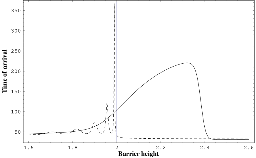
FIG. 1.: Average time of arrival at the other side of a barrier of fixed width $a=15$ as a function of the barrier momentum $p_{V}$. The parameters of the initial Gaussian wave packet are $q_{0}=-30,p_{0}=2,\delta=10,m=1$, and the arrival at $x=50$, in units with $\hbar=1$. The solid line is the quantum average (57), the dashed line is the phase time with momentum $p_{0}$. The asymptote to the left ($p_{V}\rightarrow 0$) is the time of arrival for free particles ($t_{0}=40$), the one to the right is the Hartman time $t_{H}(a)=t_{0}-\frac{m\,a}{p_{0}}=32.5$.

We show the time of arrival at the other side of a barrier of momentum $p_{V}$ in the range $a=(1.6,2.6)$ in Fig. 1. For incident plane waves with momentum $p_{0}$, the barrier would be crossed over for $p_{V}<p_{0}$, and tunneled through for $p_{V}>p_{0}$. Some retardation would be expected in the first case, just because the travel over the barrier would be slowlier than the free travel. This is clearly seen at the left of $p_{0}$ in the figure. Classically, the delay would grow from zero (time $t_{0}$) to infinity as $p_{V}$ grows from $0$ to $p_{0}$. The quantum behaviour is similar, with the oscillations of the phase time swept away by the average that remains finite. To the right of $p_{0}$, there is a dramatic difference between the Wigner result, that inmediately sticks to the Hartman prediction $t_{H}$, and the wave packet result, for which the time continues to increase up to a certain barrier height and then, suddenly, drops to $t_{H}$. This strange behaviour can be explained in the following manner: Not being monoenergetic, the wave packet has momentum components above and below $p_{V}$. The first of these cross above the barrier, get retarded, and are responsible for the high time value for $p_{V}$ just to the right of $p_{0}$. However, as the barrier continues to grow, they become an ever lesser part of the packet. The other parts of the packet (the components with momentum $p<p_{V}$) tunnel through the barrier, and experience the Hartman advance. They would arrive at $x$ in a time $t_{H}$. Their relative importance in the wave packet increases steadily as $p_{V}$ continues to grow and, eventually, they overcome the retarded components and the process becomes pure tunneling. Then, the time of arrival drops to $t_{H}$. We have numerically checked this behaviour, that we have analyzed for several values of the barrier width in the range (2,30). All the results are similar: Monotonic grow of the time from $p_{V}=0$ (where $t=t_{0}$), up to $p_{V}\approx 2.5$, where $t$ drops suddenly to $t_{H}$. The general trend is a slow increase in the value of the barrier momentum $p_{V}$ at which the drop takes place, that shifts from about 2.2 to 2.7 as $a$ changes from 10 to 30. The maximum value of the time of arrival $\langle t_{x}\rangle$ that is obtained just before the drop also increases; it is around 95 for $a=10$ and around 450 for $a=20$.

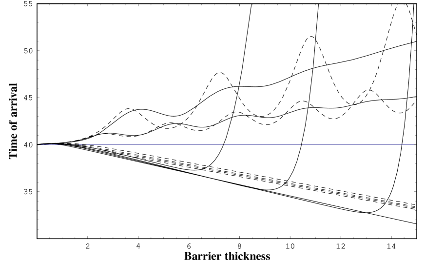
FIG. 2.: Average times of arrival at the other side of a barrier as a function of the barrier width $a$. The initial wave packet is the same as in Fig.1, and again $x=50$. We show the predictions for $p_{V}=0,1.6,1.8,2.2,2.3,2.4,2.6$. The solid lines are the quantum averages (57), the dashed lines are the corresponding Wigner times for a particle with momentum $p_{0}$

We show in Fig. 2 the average time of arrival and the Wigner (phase) time as a function of the barrier width $a$ in the range $a=(0,15)$. We display the predictions for different barrier heights $p_{V}=0,1.6,1.8,2.2,2.3,2.4$ and $2.6$. For the free case ($p_{V}=0$, or $a=0$) all the results converge to $t_{0}=40$. We now disscuss the solid lines $\langle t_{x}\rangle$. The oscillatory curves above $t_{0}$ correspond to $p_{V}<p_{0}$. The get steeper as their momenta approach $p_{0}$ from below. The curves that stand partially below $t_{0}$ correspond to $p_{V}>p_{0}$ (tunneling). They share a similar behaviour: As the barrier width grows from $a=0$ the time of arrival decreases, practically saturating the Hartman time $t(a)\approx t_{H}(a)=t_{0}-\frac{m\,a}{p_{0}}$. Then suddenly, at a certain width (that increases with $p_{V}$), the average time jumps dramatically to values that correspond to a long retardation. Note that the jump for $p_{V}=2.6$ lies outside the range of the figure. This behaviour is complementary to that shown in Fig. 1. Here, for $p_{V}>p_{0}$ and moderate $a$, tunneling is the dominant phenomenon and the time average tends to reproduce $t_{H}$. However, as the barrier gets wider, tunneling gets more and more depressed. In comparison, the intensity of the retarded components that pass over the barrier is basically independent of $a$. They get relatively more and more important and, eventually overcome tunneling, giving rise to the observed transition. In practice, for wide enough barriers, the probability of tunneling vanishes, and the other side can be reached only by the very improbable and very slow travel over the barrier. This behaviour has been noticed independently in [34], and explained in the same way. In addition, we have the tools to check these explanations. In particular, the first product of our formalism is $P(t,x)$, the probability distribution in times of arrival at $x$. Our numerical analysis for $x=50$ and the different $p_{V}$’s and $a$’s that we are discussing here show similar almost Gaussian shapes for these distributions, as correspond to the initial wave packets chosen, and similar widths for these $P(t,x)$, whose maxima are placed close to the corresponding mean values $\langle t_{x}\rangle$. As expected, the probabilities get numerically smaller as the corresponding events become more and more unlikely. In short, these distributions give the best support for the validity of the explanation offered here for this striking behaviour, that can be understood only after weighting the obtained time of arrival with the relative probability of the actual event to which it corresponds.

V Quantum reflections

Having analyzed the modifications introduced by the transmission phenomena in the time of arrival at the other side of potential barriers, we turn to the case of reflection. We divide the analysis into the two seemingly different cases in which there is classical reflection, and in which it is absent. The first case is characterized by the presence of at least one turning point in the path of the particle. The second one, by the absence of any of them. Quantum mechanically there could be some transmission in the first case, and some reflection in the second one. Accordingly, we separate the disscussion that follows into the two main disjoint cases that cover all the possibilities. These are the case where the potential energy grows to infinity somewhere (total reflection), and the case where it is bounded everywhere (with partial reflection and transmission).

A The case of total reflection

The potential energy could grow unbound, thus reflecting any conceivable incoming state. We consider here a monotonic potential energy that vanishes for $q\to-\infty$ and goes to infinity for $q\to\infty$ so that $\lim_{q\to+\infty}\langle q|E\rangle=0$. This removes the degeneracy of the energy eigenstates. As no state may arrive from the right, $\langle q|El(+)\rangle=0$. The eigenstates $|E\rangle$ will contain the same amount of positive and negative momenta, so that their asymptotic form normalized to one traveling particle per unit time is $\lim_{q\to-\infty}\langle q|E\rangle=\frac{1}{\sqrt{2\pi}}(\frac{m}{2E})^{1/4}\cos(pq+\delta(E))$, where $\delta(E)$ is the phase shift. This also fixes completely the eigenstates for finite values of $q$.

The time of arrival at an arbitrary point $x$ is now

$$\langle\psi|{\bf t}_{x}|\psi\rangle= \frac{2\pi}{P(x)}\int dE\;\sqrt{\frac{2E}{m}}\;|\langle x|E\rangle\;\langle E|\psi\rangle|^{2}\;\times$$ (59)

$$\frac{d}{dE}\{\arg\langle x|E\rangle+\arg\langle E|\psi\rangle\}$$ (60)

which is the average of a quantity independent of $x$! This comes about because in the present situation the reflection coefficient $R=\exp(-2i\delta)$ is unimodular. Then, the net current density vanishes, so that $\arg\langle x|E\rangle$ is independent of $x$. This is the quantum version of the classical result that the sum of the times of arrival at $x$ of the incoming and returning particles is twice the toa at the turning point and so, independent of $x$. Obviously this ceases when $|R|$ becomes smaller than 1 (so that the net current density is finite), something that is possible only when $V$ is finite everywhere. Even then, the classical result is recovered from the quantum case in the limit $(E/V)<<1$ where $|R|\to 1$.

The individual times of arrival of the incoming and the returning particles can be obtained straightforwardly by writing the enegy eigenstates as

$$\langle q|E\rangle=\frac{1}{\sqrt{2\pi}}(\frac{m}{2E})^{1/4}\;M(q,E)\;\cos\phi(q,E)$$ (61)

where $M$ is a real function with $\lim_{q\to-\infty}M(q,E)=1$, that vanishes faster than an exponential for $q\to+\infty$ to satisfy the asymptotic form of the Schrödinger equation. The state is thus written as the superposition at each point of an incoming and a reflected wave with equal amplitudes, so that the net current vanishes everywhere. The phase $\phi$ is fixed by $\lim_{q\to-\infty}\phi(q,E)=pq+\delta(E)$ to match the asymptotic form of the eigenstate disscussed above. Its derivative gives the two opposite velocity fields $v_{\pm}(q,E)=\pm\frac{d\phi(q,E)}{m\,dq}$ interfering at $q$. We recall that this exact expression is valid for all the potentials of the form we are considering here. The probability of ever arriving at $x$ and the toa can be given by straightforward application of (26) and (30) by

$$P(x) = \int dE\;M^{2}(x,E)\cos^{2}\phi(x,E)|\langle E|\psi\rangle|^{2}$$ (62)

$$\langle\psi|{\bf t}_{x}|\psi\rangle = \frac{1}{2P(x)}\int dE\;M^{2}(x,E)\cos^{2}\phi(x,E)\;\times$$ (64)

$$|\langle E|\psi\rangle|^{2}\;\left[t_{i}(x,E)+t_{r}(x,E)\right]$$

which is the weighted average over energies of the times of arrival of the incoming and the reflected waves:

$$t_{i}(x,E) = \frac{d}{dE}\{\phi(x,E)+\arg\langle E|\psi\rangle\}$$ (65)

$$t_{r}(x,E) = \frac{d}{dE}\{-\phi(x,E)+\arg\langle E|\psi\rangle\}$$ (66)

whose sum is explicitly $x$ independent.

To illustrate these results we consider now the case of a potential that vanishes at the left of the origin and is linear at the right, i.e. $V(q)=\theta(q)fq$, where $f$ is the force exerted on the particle. This could be a model for a (charged) particle in a constant electric field, or in the gravity field of the Earth. In this case one gets $M$ and $\phi$ in terms of the Airy function Ai and its derivativeAi’.

$$M(q,E)=\left\{\begin{array}[]{rr}1&\;\;\;\;\mbox{for}\,\,\,q\leq 0\\ \sqrt{\frac{\mbox{Ai}[z]^{2}+(\frac{k_{f}}{p})^{2}\mbox{Ai'}[z]^{2}}{\mbox{Ai}[z_{0}]^{2}+(\frac{k_{f}}{p})^{2}\mbox{Ai'}[z_{0}]^{2}}}&\;\;\;\;\mbox{for}\,\,\,q>0\end{array}\right.$$ (67)

where $z=k_{f}q-p^{2}/k_{f}^{2},z_{0}=-p^{2}/k_{f}^{2}$ with $k_{f}=(2mf)^{1/3}$. For the phase one has

$$\phi(q,E)=\left\{\begin{array}[]{rr}\arctan(-\frac{k_{f}\mbox{Ai'}[z_{0}]}{p\,\,\,\mbox{Ai}[z_{0}]}\,)&\mbox{\,\,\,for}\,\,\,q\leq 0\\ \arctan(-\frac{k_{f}\mbox{Ai'}[z]}{p\,\,\,\mbox{Ai}[z]}\,)&\mbox{\,\,\,\,for}\,\,\,q>0\end{array}\right.$$ (68)

so the phase shift is given simply by $\delta(E)=\phi(0,E)$.

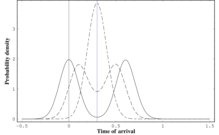
FIG. 3.: Probability distribution $P(t,x)$ in times of arrival at $x$, for $x=q_{0}$ (solid line), $x=0.5\,q_{0}$ (dashed line) and at the classical turning point $x=E/f$ (dot-dashed line). The vertical lines correspond to $t=0$ and to the classical turning time respectively. The distributions are bimodal, with the two peaks corresponding to incidence and reflection getting closer as $x$ approaches the turning point.

We present in Figures 3 and 4 our results for the the case of a force of nominal value $f=100$, being the parameters of the initial Gaussian wave packet (31) $q_{0}=-2,p_{0}=10,\delta=1$ and $m=1$. For the normalized probability distributions in times of arrival (23) we get pairs of peaks of equal heights - as correspond to total reflection - that tend to merge into one as the detector is displaced towards the classical turning point. This behaviour of the peaks is also observed for the averaged times of arrival, that follow the classical times. The small deviations from the parabolic form are negligible in comparison with the widths of the distributions shown in Fig. 3. We have explored numerically the details that change uninterestingly according to the values of $f,p_{0},\delta$ etc. so, we do not show them here. The general picture is always the same: at the far left ($|q_{0}|>>E/f$) the potential acts as an infinite height wall. The only sizeable consequences of the actual strenght of the force are felt at positions between the origin and the turning point, where they resemble the classical effects. Part of this comes from the fact that here position and energy combine into only a variable $q-E/f$. But the resemblance arises because total reflection is always present here, quantum as well as classically. This will be more clear in the next section where we consider partial reflection that lacks of classical analog.

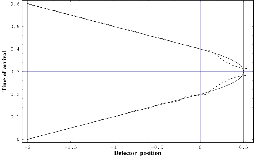
FIG. 4.: Average time of arrival for different detector positions. The vertical lines correspond to $x=q_{0},\;\;x=0$ and $x=E/f$ respectively. The solid line is the classical time, the dashed line is the quantum average of $t_{i}$ (lower part) and of $t_{r}$ (upper part).

B Partial reflections

In classical mechanics a potential interaction energy speeds up or slows down the particles according to the local value of the force $F(q)=-\frac{\partial V(q)}{\partial q}$. Accelerated or decelerated, the particles continue to move along the same path without reversing the direction. Only when one of them intercepts a turning point (i.e. a point $q$ where $E=V(q)$) the particle bounces back or, in other words, is reflected with probability $P_{R}=1$. In the absence of these points, the particle is always transmitted with probability $P_{T}=1$. Thus, most of the time $P_{T}=1,P_{R}=0$. Only at the turning points $P_{T}=0,P_{R}=1$.

Quantum dynamics offers a very different perspective of the motion of the particles. The Schrödinger equation implies that at every point where the potential energy is finite, the particle is partially transmitted and partially reflected, that is $0\leq P_{T}\leq 1,0\leq P_{R}\leq 1$, with $P_{T}+P_{R}=1$. The case of total reflection analyzed in the previous section is one of close correspondence between the classical and the quantum results, as we shown there. Interesting departures from the classical behaviour arise when there is no classical reflection. We will analyze this case here.

To fix ideas, we consider a well behaved potential energy $V(q)\geq 0\;\forall$ finite $q$, that vanishes at the spatial infinity faster than $q^{-1}$. In these conditions the energy eigenstates can be written everywhere as a well defined superposition of transmitted $\Phi_{tr}(q,E)$ and reflected $\Phi_{ref}(q,E)$ waves, characterized by the positive or negative value of their currents: $-\frac{i}{2m}(\Phi_{tr}^{*}\stackrel{{\scriptstyle\leftrightarrow}}{{\frac{d}{dq}}}\Phi_{tr})\geq 0$, and $-\frac{i}{2m}(\Phi_{ref}^{*}\stackrel{{\scriptstyle\leftrightarrow}}{{\frac{d}{dq}}}\Phi_{ref})\leq 0$, with different amplitudes $|\Phi_{tr}|\neq|\Phi_{ref}|$ as corresponds to this case of partial reflection. The eigenstates of interest can be written as

$$\langle q|E\,r\rangle=\sqrt{\frac{m}{2\pi p}}\{\Phi_{tr}(q,E)+\Phi_{ref}(q,E)\}$$ (69)

These waves are univocally determined by their asymptotic conditions, namely:

$$\lim_{q\to-\infty}\Phi_{tr}(q,E)= e^{ipq}, \lim_{q\to+\infty}\Phi_{tr}(q,E)=T(E)e^{ipq}$$ (70)

$$\lim_{q\to-\infty}\Phi_{ref}(q,E)= R(E)e^{-i(pq+2\delta(E))}, \lim_{q\to+\infty}\Phi_{ref}(q,E)=0$$ (71)

as is the case for an incoming rightmover (69). The results of the previous section are recovered in the limit where $T(E)\rightarrow 0$ which is the case only if the potential energy grows to infinity somewhere.

If we prepare our initial Gaussian state $\psi(q)$ at a point $q=q_{0}$ where the potential energy is smooth enough, and keep the initial momentum $p_{0}>0$ large enough to consider $\tilde{\psi}(p)\approx 0$ for $p<0$, we can use the approximations

$$\langle E\,s|\psi\rangle\approx\delta_{rs}\sqrt{\frac{m}{p}}\;\Phi_{tr}^{*}(q_{0},E)\;|\tilde{\psi}(p)|\approx\delta_{rs}\sqrt{\frac{m}{p}}\;e^{-ipq_{0}}\;|\tilde{\psi}(p)|$$ (72)

We have used the second of these already in Eq.(33). It is valid when $V(q)\approx 0$ for $q$ in the $q_{0}$ neighbourhood where $\psi(q)$ is sizeable. We assume this is the case in what follows.

One of the deepest consequences of the superposition of transmitted and reflected components that makes up the eigenstate (69) is that it leads to the inescapable presence of interferences. In fact, the probability of presence at a point $q$, and other quantities depending on it, contain the sum $|\langle q|Er\rangle|^{2}\propto|\Phi_{tr}|^{2}+|\Phi_{ref}|^{2}+2\Re(\Phi_{tr}\Phi_{ref}^{*})$, whose last term is the interference term. One could say that, everywhere in its motion through the interaction region, the quantum particle will be found in an evolving entangled state of transmitted and reflected components. This can be traced back mathematically to the continuity of the solutions of the Schrödinger equation and of their first derivatives, and to the associated Wronskian theorem. Physically, this may introduce all sorts of interpretative difficulties in the analysis of particle motion.

Summarizing, interferences pervade the realm of quantum motion. They will show up in almost every quantum mechanical situation. Our analysis of the time of arrival is not an exception. We have avoided refering to them till now by focusing on very specific cases. These were: The choice in Sect. 3.1. of a very smooth potential analyzable semiclassically by the WKB method, that neglects reflection. The analysis in Sect. 3.3. of the time of arrival at points located at the other side of the barrier, where $\Phi_{ref}=0$ so that any interference with the transmitted wave vanishes. Finally, the analysis made in the previous section, where we just ignored the effects due to the overlap of incoming and reflected waves in $P(t,x)$, and the lack of a clear cut separation between $t_{i}$ and $t_{r}$ in the presence of interferences. To be precise, we dealt with reflection without paying the due attention to these subtleties. We repair the ommission here.

The amplitude in time of arrival at a position $x$ within the interaction range can be given by using (69) and (72) in (48)

$$\langle txs|\psi\rangle = \{A_{tr}(t,x)+A_{ref}(t,x)\}$$ (73)

$$\approx \frac{\delta_{sr}}{\sqrt{2\pi}}\int_{0}^{\infty}dp\sqrt{\frac{p}{m}}\;|\tilde{\psi}(p)|\;e^{-i(Et+pq_{0})}\;\{\Phi_{tr}(x,E)+\Phi_{ref}(x,E)\}$$ (74)

This gives for the probability of ever arriving at $x$ Eq. (26) the sum of three terms: The two separated probabilities $P_{tr},P_{ref}$ of arriving with positive or with negative current density, and a quantum interference term, whose presence deprives the previous two of direct physical meaning. We thus get $P(x)=P_{tr}(x)+P_{ref}(x)+I(x)$ with

$$P_{{}_{tr\atop ref}}(x)=\int dt\;|A_{{}_{tr\atop ref}}(t,x)|^{2}\approx\int dp\;|\tilde{\psi}(p)|^{2}|\Phi_{{}_{tr\atop ref}}(x,E)|^{2}$$ (75)

and an interference term

$$I(x) = 2\int dt\;\Re\{A_{tr}(t,x)\,A^{*}_{ref}(t,x)\}$$ (76)

$$\approx 2\int dp\;|\tilde{\psi}(p)|^{2}\Re\{e^{-ipq_{0}}\;\Phi_{tr}(x,E)\;\Phi_{ref}(x,E)^{*}\}$$ (77)

The above quantities depend on the probabilities of transmission or reflection from the initial position $q_{0}$ to the actual value $x$. Consider a bounded potential barrier of finite range, but otherwise arbitrary. Behind the barrier $P_{ref}$ vanishes, while $P_{tr}$ is given by (54) with a value independent of $x$, but strongly dependent of $p_{0},\delta$ and of the barrier’s height and width. For $x$ at the left of the barrier $\Phi_{tr}=e^{ipx}$ (what we are denoting as transmission is here incidence), but $\Phi_{ref}=R(E)\,e^{-i(px+2\delta(E))},$ and only when there is no reflection (no barrier) the intereferences dissappear. For the total reflection case of the previous section, we get $P_{tr}=P_{ref}$, while the interference term gives rise to the term $\cos\{2(px+\delta(E))\}$ that builds up the factor $\cos^{2}\phi$ that appears in (62) and (64). However it does not prevent the definition of the quantities (65) and(66) that allowed to split the toa (64) into two positive contributions interpretable as the independent $\langle t_{x}\rangle$ of an incoming packet and a reflected one (Fig. 4).

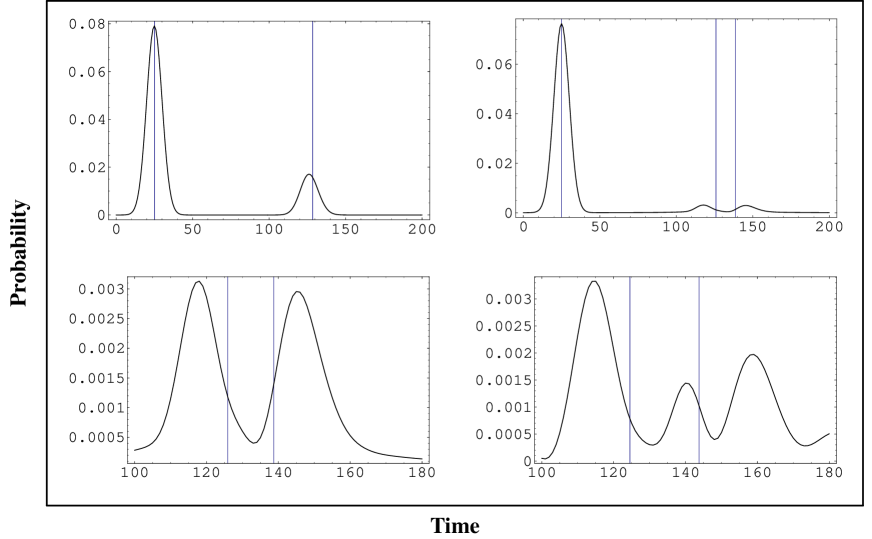
FIG. 5.: Probability distribution $P(t,x)$ in times of arrival for reflection from finite potential barriers. The initial wave packet is the Gaussian one with $m=1,p_{0}=2,\delta=10$, placed at $q_{0}=-150$. The arrival position is at $x=-100$. The upper left figure is for a barrier width $a=4$ and $p_{V}=2.2$. At its right is the case $a=4$ and $p_{V}=1.9$, that is enlarged in the lower left part for the range $t=[100,180]$. An illustrative case of multimodal reflection distribution is shown at the lower right part, that corresponds to $p_{V}=1.9$ and $a=6$. The vertical grid lines correspond to the phase times of the incident wave $e^{ip_{0}x}$ and of the reflected waves: $e^{-ip_{0}x}$ for $p_{V}>p_{0}$, and the superposition $\sin p_{0}^{\prime}a\;e^{-ip_{0}x}$ for $p_{V}<p_{0}$.

For finite barriers reflection is always present with an energy dependent coefficient $R(E)<1$; it is less probable than incidence, and tends to vanish as the barrier does. In Fig. 5 we give the probability distributions of toa $P(t,x)$ at a point $x$, whose bumps indicate, as in Fig. 3, the arrival of incident and reflected parts of the time evolved initial wave packet. This is the Gaussian one with $m=1,p_{0}=2,\delta=10$, placed at $q_{0}=-150$. The arrival position is at $x=-100$, far from $q_{0}$ to avoid interferences. The two upper figures are for a barrier of width $a=4$. At the left is the case where $p_{V}=2.2$, and at the right that with $p_{V}=1.9$. In both cases there is an incidence bump centered at $t=m(x-q_{0})/p_{0}=25$, and a structure to its right corresponding to reflection. For $p_{V}=2.2$, and for all the cases of total classical reflection ($p_{V}>p_{0}$), the latter is a Gaussian-like bump shifted from the classical value at $t=m(-x-q_{0})/p_{0}=125$ by an amount $\langle\frac{m}{p}(\frac{d\phi}{dp})\rangle$. However, for $p_{V}=1.9$ (in general for $p_{V}<p_{0}$), the reflected distribution has a multi-bump shape difficult to understand in terms of the phase time or of any other approximation. In particular, neither the number of peaks, nor their positions heights and widths can be approximated by straight stationary phase methods. Two illustrative cases of these shapes are shown in some detail in the two examples of the lower part that correspond to $p_{V}=1.9$ and two close widths $a=4$ and $a=6$.

VI Conclusions

We have worked out a formalism for obtaining the time of arrival at a space point of particles that move through interacting media. Our construction follows a circuitous path: we desist from first computing the classical toa of the problem, and then quantizing it, a procedure that leads to a dead end. Instead, we start from the quantum toa of the free moving particle, and then transform it canonically to the interacting case. This is achieved by the use of the appropriate Möller operator that implements the quantum version of the Jacobi-Lie canonical transformation to free translation coordinates in phase space. In the classical case we have the transformation of Eq. (82) whose quantum counterpart is

$$\{{\cal H},H\}\stackrel{{\scriptstyle\Omega^{\dagger}}}{{\longrightarrow}}\{{\cal H}_{0},H_{0}\}$$ (78)

where ${\cal H}_{0}$ and ${\cal H}$ are the Hilbert spaces of the free and interacting particles, and $H_{0},H$ the respective Hamiltonian operators in these spaces. For simplicity, we have only addressed explicitly cases in which the transformations are unitary, which is the case when $\sigma(H)=\sigma(H_{0})$. More general situations that require of isometric transformations, deserve a separate treatment by their physical relevance.

What we obtained here is a quantum formalism for the toa in terms of a POVM given by

$$P(t_{1},t_{2};x)=\sum_{s=r,l}\int_{t_{1}}^{t_{2}}dt\;|t\ x\ s\rangle\langle t\ x\ s|$$ (79)

which measures the probability of arrival at $x$ during the time interval $(t_{1},t_{2})$. The normalized probability distribution $P(t,x)$ was given in the Eq. (23) of Sect. II.B. Our results are thus within the standard formalism of quantum mechanics and can be interpreted in the standard way. There is nothing special that singles out our theoretical predictions as unsuitable for comparison with the experimental results. On the contrary, our formalism predicts the result of actual experiments in the form of numeric values and statistics for the recorded events.

After the definition and theoretical analysis of Sect. II. we have performed explicit and complete calculations for the cases of an unbounded linear potential, of the step potential and of the square barrier. Our analysis of the quasi-classical case shows that in this limit the toa is simply given by the average of the classical time of Eq. (1) over the quasi-classical wave function. In the case of reflection, and for the arrival point placed between the initial position of the wave packet and the turning point ($x<0$), the probability distribution $P(t,x)$ is governed by the quantum superposition of the incident $(A_{tr})$ and the reflected $(A_{ref})$ wave packets. In the case of total reflection, where both are equally probable $P_{tr}(x)=P_{ref}(x)$, we have obtained separate positive $\langle t_{x}\rangle$ even when both amplitudes overlap. These were interpreted as the toa’s of the incident and reflected particles, and compared successfully with the classical prediction. For partial reflection, $P_{ref}(x)<P_{tr}(x)$ non overlapping amplitudes are necessary to to get separate average values for these times. This problem is shared with the position and other operators. It is not a defect of the formalism, but an effect of the interferences. Fortunately enough, our formalism provides us with the probability distribution $P(t,x)$ whose diverse humpy-bumpy shapes (Figs. 3 and 5) give the most complete information of the posible experimental outcomes.

In the course of our numerical analysis we have detected that the phase time $\tau_{\phi}$ not always gives a good approximation to the most probable time of arrival. It provides a first estimate of the time spent in the transmission or reflection, after substracting the time of free flight. For transmitted wave packets we have reobtained the advancement (i.e. a decrease in the toa) in the case of pure quantum tunneling. This phenomenon, predicted by Hartman long time ago [22], has been experimentally evinced by the two photon experiments at Berkeley [19, 20] and the tunneling of optical pulses at Wien [21]. However, our formalism predicts a striking departure from the Hartman bound that we explain in detail in Sect. IV. Our results for square barriers neatly show the expected advancement roughly proportional to the width $\Delta t=-ma/p$ (Figs. 1 and 2). However, whatever the mean energy $(E<V)$ of the incident wave packet, there is always a width $a_{0}$ such that for $a>a_{0}$ the (very retarded) components of the packet that stand above the barrier dominate over the (probabilistically very depressed) tunneled ones, giving an overall effective strong retardation. In other words, when the barrier is wide enough, its width dominates over the Hartman lenght $\Delta x$ disscussed above Eq. (47), that has a purely quantum origin. This restores the classical expectation of no tunneling and very long delays.

We have also found other unanticipated phenomenon for purely quantum reflection: the multiple bump structure that appears when $p_{V}<p_{0}$. We have shown in Fig. 5 this structure, that in some sense is a counterpart of the interference pattern that appears in multiple reflection of stationary waves. We think that this feature, even if less spectacular than the superluminal tunneling of photons, deserves experimental confirmation. An appropriate modification of the two photon experiments could serve for this purpose. It would require to place a quantum mirror in the path of one of the entangled photons, and check for the presence (or absence) of the multiple dip structure in the number of coincidence counts predicted by the formalism.

All the examples above show that our construction of a quantum toa operator suitable for the presence of interactions allows the exploration of many physical details in relevant situations. Its extension to higher dimensional cases poses no conceptual difficulties and opens the possibility of treating new questions. Of great theoretical and experimental interest will be the extension of this formalism to the cases in which the Hamiltonian has bound states, where isometric (instead of simply unitary) transformations will be requiered.

Appendix A

In the modern literature [38], a classical Hamiltonian system with $n$ degrees of freedom is called completely integrable ( a là liouville) when it satisfies the conditions $a$ and $b$ below:

• There are $n$ compatible conservation laws $\Phi_{i}(q_{1},\ldots,q_{n},p_{1}\ldots,p_{n};t)=C_{i}$, $i=1,\ldots,n$, that is:

  • $\dot{\Phi}_{i}=\{\Phi_{i},H\}+\frac{\partial\Phi_{i}}{\partial t}=0,\;\forall\;i=1,\ldots,n.$

  • $\{\Phi_{i},\Phi_{j}\}=0,\;\forall\;i,j=1,\ldots,n.$

• The conservation laws define $n$ isolating integrals that can be written as:

  • $\Phi_{i}=C_{i}\Rightarrow p_{i}=\phi_{i}(q_{1},\ldots,q_{n},C_{1},\ldots,C_{n};t),\;\forall\;i=1,\ldots,n.$

  • $\frac{\partial\phi_{i}}{\partial q_{j}}=\frac{\partial\phi_{j}}{\partial q_{i}}\,\;\forall\;i,j=1,\ldots,n.$

In these conditions, Hamilton equations define an integrable flow, that is, a system of holonomic coordinates $(q(t),p(t))$ in phase space for each instant of time:

$$q_{i}(t) =q_{i}(q_{0},p_{0};t), \;\;i=1,\ldots,n.$$ (80)

$$p_{i}(t) =p_{i}(q_{0},p_{0};t), \;\;i=1,\ldots,n.$$ (81)

In other words, given a set of initial conditions $(q_{0},p_{0})$ of the system, at each instant of time $t$ the system arrives at a point $(q(t),p(t))$ in phase space. Conversely, these points define the corresponding times of arrival. In this case, time meets the requirements to qualify as a derived variable in phase space.

As Lie pointed out, for any arbitrary time there is a special choice of coordinates in phase space that mathematically eliminates the effects of interactions from these integrable flows, (the new positions are ignorable coordinates). More simply, integrable systems are canonically equivalent to a set of translations (or circular motions) at constant speed. It is customary to denote the variables that determine these translations as action-angle variables, which strictly is appropriate only in the case of periodic systems, where the (closed) flow lines are topologically equivalent to circles.

For integrable flows, there is a canonical transformation (the Jacobi-Lie transformation)

$$\{q,p;H(q,p)\}\stackrel{{\scriptstyle W(q,P)}}{{\longrightarrow}}\{Q,P;\bar{H}(Q,P)\}$$ (82)

with $H(q,p)=\bar{H}(Q,P)$, that gives the free translation coordinates $P(t)=P$, and $Q(t)=\frac{P}{m}t+Q$ of the translation flow with $\bar{H}(Q,P)=\frac{P^{2}}{2m}$, in terms of the coordinates and momenta $(q(t),p(t))$ of the actual flow with $H(q,p)=\frac{p^{2}}{2m}+V(q)$. This transformation is of the form $W(q,P)$, that is, a function of the old coordinates and the new momenta, so that

$$Q=\frac{\partial W}{\partial P},\;\;p=\frac{\partial W}{\partial q}$$ (83)

Finally, $W$ can be obtained explicitly as a complete integral of the Hamilton-Jacobi equation:

$$H(q,\frac{\partial W}{\partial q})=\frac{P^{2}}{2m}$$ (84)

Now, the canonical relation among the new and the old variables is:

$$P = \mbox{sign}(p)\sqrt{2m\;H(q,p)}$$ (85)

$$Q = \int_{0}^{q}\frac{dq^{\prime}}{\sqrt{1-\frac{V(q^{\prime})}{H(q,p)}}}+Q_{0}$$ (86)

where $Q_{0}$ is a constant. As a byproduct, time gets defined in equivalent manner in terms of the old variables, or of the new ones. If the particle arrives at $q(t)=x$ in the instant $t(x)=t$, then:

$$t(x)=\frac{m}{P}(X-Q)=\mbox{sign}(p)\int_{q}^{x}\frac{m\;dq^{\prime}}{\sqrt{2m\,(H(q,p)-V(q^{\prime}))}}$$ (87)

where $X=\partial W(x,P)/\partial P$ (obviously, $X=Q(t)$ by construction). This duality, devoid of practical interest in the classical domain, is at the foundations of the quantum method developed in this paper. Finally, note that for simplicity we have specialized the notation to the case of autonomous Hamiltonian systems with only one degree of freedom, all of them trivially integrable ($H(q,p)=E$ being the needed conserved quantity).

Appendix B

For free particles Eq. (1) gives $t_{x0}(q,p)=m(x-q)/p$ that, in spite of its simplicity, presents some problems for quantization [4, 15, 17] whose solution we outline here. First of all, it requires symmetrization:

$${\bf t}_{x0}({\bf q},{\bf p})=m(\frac{x}{{\bf p}}-\frac{1}{2}\{{\bf q},\frac{1}{{\bf p}}\}_{+})=-e^{-i{\bf p}x}\sqrt{\frac{m}{{\bf p}}}{\bf q}\sqrt{\frac{m}{{\bf p}}}e^{i{\bf p}x}$$ (88)

As is well known, the eigenstates $|txs0\rangle$ of this operator in the momentum representation can be given as ($\hbar=1$)

$$\langle p|txs0\rangle=\theta(sp)\sqrt{\frac{|p|}{m}}\,\exp(i\frac{p^{2}}{2m}t)\,\langle p|x\rangle$$ (89)

where we use $s=r$ for right-movers ($p>0$), and $s=l$ for left movers ($p<0$.) The label $0$ stands for free case. Finally, the argument $sp$ of the step function that appears in the momentum representation is $+p$ for $s=r$, and $-p$ for $s=l$. The degeneracy of the energy with respect to the sign of the moment is explicitly shown by means of the label $s$ in the energy representation, where

$$\langle Es^{\prime}0|txs0\rangle=\delta_{s^{\prime}s}\,(\frac{2E}{m})^{1/4}e^{iEt}\,\langle Es0|x\rangle$$ (90)

Summarizing, there is a time (of arrival at $x$) representation spanned by the eigenstates

$$|txs0\rangle=(\frac{2H_{0}}{m})^{1/4}e^{iH_{0}t}\Pi_{s0}|x\rangle$$ (91)

where $\Pi_{s0}$ projects on the subspace of right-movers ($s=r$), or left-movers ($s=l$), i.e.

$$\Pi_{s0}=\int_{0}^{\infty}dE|Es0\rangle\langle Es0|$$ (92)

These time eigenstates are not orthogonal, which in the past gave rise to serious doubts about their physical meaning. The origin of this problem can be traced back to the fact that (88) is not self-adjoint, that is $\langle\varphi|{\bf t}_{x0}\psi\rangle\neq\langle{\bf t}_{x0}\varphi|\psi\rangle$. This was proved by Pauli [2] long time ago and is due to the lower bound on the energy spectrum. The problem emerges as soon as one attempts integration by parts in the energy representation. Ref. [28] is a recent illuminating review of these and other related questions.

The measurement problem posed by this not self-adjoint toa operator can be solved by interpreting it in terms of a Positive Operator Valued Measure (POVM), that only requires the hermiticity of ${\bf t}_{x0}$ (i.e. ${\bf t}_{x0}={({\bf t}_{x0})^{*}}^{\top}$). Here, instead of a Projector Valued spectral decomposition of the identity operator, one has the POVM

$$P_{0}(\Pi(x);t_{1},t_{2}) = \sum_{s}\int_{1}^{2}dt\,|txs0\rangle\,\langle txs0|$$ (93)

$$= \sum_{s}\int_{1}^{2}dt\,(\frac{2H_{0}}{m})^{1/4}\,e^{iH_{0}t}\,\Pi_{s0}\,\Pi(x)\,\Pi_{s0}\,e^{-iH_{0}t}\,(\frac{2H_{0}}{m})^{1/4}$$ (94)

where $\Pi(x)=|x\rangle\,\langle x|$ is the projector on $x$. Here, $P_{0}(1,2)^{2}\neq P_{0}(1,2)$ because $|txs0\rangle\langle txs0|$ is not a projector, as the states are not orthogonal, but where the limit as $t\rightarrow\infty$ of $P_{0}(-t,+t)$ is the identity. The attained time operator is no longer sharp, but is well suited for measurement. This solution has been implemented in [18], and extensively analyzed in refs.  [35, 36] and in the review [28]. In this POVM formulation the toa is given by the spectral decomposition

$${\bf t}_{0}(H_{0},\Pi(x))=\int_{-\infty}^{+\infty}dt\,t\,(\frac{2H_{0}}{m})^{1/4}\,e^{iH_{0}t}\,{\cal P}_{0}(x)\,e^{-iH_{0}t}\,(\frac{2H_{0}}{m})^{1/4}$$ (95)

where ${\cal P}_{0}(x)=\sum_{s}\Pi_{s0}\,\Pi(x)\,\Pi_{s0}$, which is not a projector.

REFERENCES

- [1] e-mail addresses: julve@imaff.cfmac..csic.es, leon@imaff.cfmac.csic.es, pitanga@if.ufrj.br and fernando.urries@alcala.es.
- [2] W. Pauli, in Encyclopedia of Physics Vol. 5, ed. S. Flugge, Springer, Berlin 1958.
- [3] L. Mandelstamm and I. Tamm, J. Phys. USSR 9 (1945) 249.
- [4] Y. Aharonov and D. Bohm, Phys. Rev. 122 (1961) 1649.
- [5] V. A. Fock, Soviet Phys. JETP, 15 (1962) 784.
- [6] Y. Aharonov and D. Bohm, Phys. Rev. 134 (1964) B1417.
- [7] P. Busch, Found. Phys. 20 (1990) 1; ibid 20 (1990) 33.
- [8] J. Hilgevoord, Am. J. Phys. 64 (1996) 1451; ibid 66 (1998) 396.
- [9] C. J. Isham, in Integrable Systems, Quantum Groups, and Quantum Field Theory, L. A. Ibort and M. A. Rodriguez, eds, Kluwer, London (1993).
- [10] G. R. Allcock, Ann. Phys. NY 53 (1969) 253; ibid 53 (1969) 286; ibid 53 (1969)311.
- [11] Y. Aharonov, J. Oppenheim, S. Popescu, B. Reznik and W. G. Unruh, Phys. Rev. A 57 (1998) 4430.
- [12] J. Oppenheim, B. Reznik and W. G. Unruh, Minimum Uncertainity for Transit Time, quant-ph/9801034, Jan 1998.
- [13] S. Brouard, D. Macías and J. G. Muga, J. Phys. A 27 (1994) L493.
- [14] J. G. Muga, J. P. Palao and C. R. Leavens, Quantum arrival time measurement and backflow effect, quant-ph/9803087, Mar 1998.
- [15] N. Grot, C. Rovelli and R. S. Tate, Phys. Rev. A 54 (1996) 4676.
- [16] V. Delgado and J. G. Muga, Phys. Rev. A 56 (1997) 3425.
- [17] J. León, J. Phys. A 30 (1997) 4791.
- [18] R. Giannitrapani, Int. Journ. Theor. Phys. 36 (1997) 1575.
- [19] A. M. Steinberg, P. G. Kwiat and R. Y. Chiao, Phys. Rev. Lett. 68 (1992) 2421.
- [20] A. M. Steinberg and R. Y. Chiao, Phys. Rev. A 51 (1995) 3525.
- [21] Ch. Spielmann, R. Szipöcs, A. Stingl and F. Krausz, Phys. Rev. Lett. 73 (1994) 2308.
- [22] T. E. Hartman, J. Appl. Phys. 33 (1962) 3427.
- [23] E. P .Wigner, Phys. Rev. 98 (1955) 145.
- [24] M. Büttiker and R. Landauer, Phys. Rev. Lett. 49 (1982) 1739.
- [25] M. Büttiker, Phys. Rev. B 27 (1983) 6178.
- [26] F. T. Smith, Phys. Rev. 118 (1960) 349.
- [27] J. G. Muga, R. Sala and J. P. Palao, Superlattices Microstruct. 23 (1998) 833.
- [28] J. G. Muga, C. R. Leavens, and J. P. Palao, Space-time properties of free motion time-of-arrival eigenstates, quant-ph/9807066, Jul 1998.
- [29] R. Y. Chiao and A. M .Steinberg. Tunneling Times and Superluminality, in E. Wolf, Progress in Optics XXXVVII. Elsevier Science B. V . 1997.
- [30] R. Y. Chiao, Tunneling Times and Superluminality: a Tutorial, quant-ph/9811019, Nov 1998.
- [31] J. León, J. Julve, P. Pitanga and F. J. de Urríes, Time of arrival through a quantum barrier, quant-ph/9903060.
- [32] P. A. M. Dirac, Phys. Z. Sowj. Band 3, Heft 1 (1933). Reprinted in “Selected papers on Quantum Electrodynamics”, Ed. J. Schwinger, Dover, New York, 1958.
- [33] M. Moshinsky and T. H. Seligman, Ann. Phys. NY 114 (1978) 243; ibid 120 (1979) 402.
- [34] K. I. Aoki, A. Horikoshi and E. Nakamura, Time of Arrival Through Interacting Environments - tunnelling case -, quant-ph/9912109.
- [35] R. Giannitrapani, J. Math. Phys. 39 (1998) 5180.
- [36] M. Toller On the Quantum Space-Time Coordinates of an Event. quant-ph/9702060 v2 13 Mar 1997.
- [37] A. M. Steinberg, Conditional probabilities in quantum mechanics theory and the tunneling time controversy quant-ph/9502003, Feb 1995.
-
[38]
V. I. Arnold, K. Vogtmann and A. Weinstein, Mathematical Methods of Classical Mechanics, Springer Verlag,
Berlin, 1989.
J. L. McCauley, Classical Mechanics, Cambridge University Press, Cambridge, 1998.