[

Inverse Time–Dependent Quantum Mechanics

Abstract

Using a Bayesian method for solving inverse quantum problems, potentials of quantum systems are reconstructed from coordinate measurements in non–stationary states. The approach is based on two basic inputs: 1. a likelihood model, providing the probabilistic description of the measurement process as given by the axioms of quantum mechanics, and 2. additional a priori information implemented in form of stochastic processes over potentials.

]

The first step to be done when applying quantum mechanics to a real world system is the reconstruction of its Hamiltonian from observational data. Such a reconstruction, also known as inverse problem, constitutes a typical example of empirical learning. Whereas the determination of potentials from spectral and from scattering data has been studied in much detail in inverse spectral and inverse scattering theory [1, 2], this Paper describes the reconstruction of potentials by measuring particle positions in coordinate space for finite quantum systems in time–dependent states. The presented method can easily be generalized to other forms of observational data.

In the last years much effort has been devoted to many other practical empirical learning problems, including, just to name a few, prediction of financial time series, medical diagnosis, and image or speech recognition. This also lead to a variety of new learning algorithms, which should in principle also be applicable to inverse quantum problems. In particular, this Paper shows how the Bayesian framework [3] can be applied to solve problems of inverse time–dependent quantum mechanics (ITDQ). The presented method generalizes a recently introduced approach for stationary quantum systems [4, 5]. Compared to stationary inverse problems, the observational data in time–dependent problems are more indirectly related to potentials, making them in general more difficult to solve.

Specifically, we will study the following type of observational data: Preparing a particle in an eigenstate of the position operator with coordinates $x_{0}$ at time $t_{0}$, we let this state evolve in time according to the rules of quantum mechanics and measure its new position at time $t_{1}$, finding a value $x_{1}$. Continuing from this measured position $x_{1}$, we measure the particle position again at time $t_{2}$, and repeat this procedure until $n$ data points $x_{i}$ at times $t_{i}$ have been collected. We thus end up with observational data of the form $D$ =$\{(x_{i},\Delta_{i},x_{i-1})|1\leq i\leq n\}$, where $x_{i}$ is the result of the $i$-th coordinate measurement, $\Delta_{i}$ = $t_{i}-t_{i-1}$ the time interval between two subsequent measurements and $x_{i-1}$ the coordinates of the previous observation (or preparation) at time $t_{i-1}$.

We will discuss in particular systems with time–independent Hamiltonians of the form $H$ = $T+V$, consisting of a standard kinetic energy term $T$ and a local potential $V(x,x^{\prime})$ = $\delta(x-x^{\prime})v(x)$, with $x$ denoting the position of the particle. In that case, the aim is the reconstruction of the function $v(x)$ from observational data $D$. (The restriction to local potentials simplifies the numerical calculations. Nonlocal Hamiltonians can be reconstructed similarly.)

Setting up a Bayesian model requires the definition of two probabilities: 1. the probability $p(D|v)$ to measure data $D$ given potential $v$, which, for $D$ considered fixed, is also known as the likelihood of $v$, and 2. a prior probability $p(v)$ implementing available a priori information concerning the potential to be reconstructed.

Referring to a maximum a posteriori approximation (MAP) we understand those potentials $v$ to be solutions of the reconstruction problem, which maximize $p(v|D)$, i.e., the posterior probability of $v$ given all available data $D$. The basic relation is then Bayes’ theorem, according to which $p(v|D)\propto p(D|v)p(v)$.

One possibility is to choose a parametric ansatz for the potential $v$. In that case, an additional prior term $p(v)$ is often not included (so the MAP becomes a maximum likelihood approximation). In the following, we concentrate on nonparametric approaches, which are less restrictive compared to their parametric counterparts. Their large flexibility, however, makes it essential to include (nonuniform) priors. Corresponding nonparametric priors are formulated explicitly in terms of the function $v(x)$ [6]. Indeed, nonparametric priors are well known from applications to regression [7], classification [8], general density estimation [9], and stationary inverse quantum problems [4, 5]. It is the likelihood model, discussed next, which is specific for ITDQ.

According to the axioms of quantum mechanics the probability that a particle is found at position $x_{i}$ at time $t_{i}$, provided the particle has been at $x_{i-1}$ at time $t_{i-1}$, is given by

$$p_{i}=p(x_{i}|\Delta_{i},x_{i-1},v)=|\phi_{i}(x_{i})|^{2},$$ (1)

where

$$\phi_{i}(x_{i})\,=\,<x_{i}\,|\,\phi_{i}\!>\,=\,<\!x_{i}|U_{i}\,x_{i-1}\!>,$$ (2)

are matrix elements of the time evolution operator

$$U_{i}=e^{-i\Delta_{i}H},$$ (3)

setting $\hbar$ = 1. The transition amplitudes (2) can be calculated by inserting orthonormalized eigenstates $\psi_{\alpha}$ of $H$, with energies $E_{\alpha}$,

$$\phi_{i}(x_{i})=\sum_{\alpha}e^{-i\Delta_{i}E_{\alpha}}\psi_{\alpha}(x_{i})\psi_{\alpha}^{*}(x_{i-1}).$$ (4)

Clearly, it is straightforward to modify (1) for measuring observables different from the particle position. It is also interesting to note that the transition probabilities (1) define a Markoff process with $W_{i}(x\rightarrow x^{\prime})$ = $p(x^{\prime}|\Delta_{i},x,v)$. For real eigenfunctions $\psi_{\alpha}(x)$, i.e., for a real Hamiltonian with real boundary conditions, they obey the relation $W_{i}(x\rightarrow x^{\prime})$ = $W_{i}(x^{\prime}\rightarrow x)$. It follows that the detailed balance condition, $p_{\rm stat}(x)W_{i}(x\rightarrow x^{\prime})$ = $p_{\rm stat}(x^{\prime})W_{i}(x^{\prime}\rightarrow x)$, is fulfilled for a uniform $p_{\rm stat}(x)$, which therefore represents the stationary state of the Markoff process of repeated position measurements.

Having defined the likelihood model of ITDQ, in the next step a prior for $v$ has to be chosen. A convenient nonparametric prior $p(v)$ is a Gaussian

$$p_{G}(v)=\left(\det\frac{{\bf K}_{0}}{2\pi}\right)^{\frac{1}{2}}e^{-\frac{1}{2}<v-v_{0}|{\bf K}_{0}|v-v_{0}>},$$ (5)

with (real symmetric, positive semi–definite) inverse covariance ${\bf K}_{0}$, acting in the space of potentials, and mean $v_{0}(x)$, which can be considered as a reference potential for $v$. Typical examples are smoothness constraints on $v$ which correspond to choosing differential operators for ${\bf K}_{0}$. Reference potentials can be made more flexible by allowing parameterized families $v_{0}(x;\theta)$. Within the context of Bayesian statistics such additional parameters $\theta$ are known as hyperparameters. In MAP approximation the optimal hyperparameters are determined by maximizing the posterior (7) simultaneously with respect to $\theta$ and $v(x)$ [10]. A simplified procedure consists in using a parametric approximation $v(\theta)$ which maximizes the likelihood $\prod_{i}p_{i}(\theta)$ as reference potential $v_{0}$ for the nonparametric reconstruction $v(x)$ [9].

If available, it is useful to include some information about the ground state energy $E_{0}(v)$, which helps to determine the depth of the potential. This can, for example, be a noisy measurement of the ground state energy which, assuming Gaussian noise, is implemented by

$$p_{E}\propto e^{-\frac{\mu}{2}\left(E_{0}(v)-\kappa\right)^{2}}.$$ (6)

Combining (5) and (6) with (1) for $n$ repeated coordinate measurements starting from an initial position $x_{0}$, we obtain for the posterior (7),

$$p(v|D)\propto p_{G}(v)\,p_{E}(v)\prod_{i=1}^{n}p_{i}.$$ (7)

To calculate the MAP solution $v^{*}$ =${\rm argmax}_{v}p(v|D)$ we set the functional derivative of the posterior (7), or technically more convenient of its logarithm, with respect to $v$, denoted $\delta_{v}$, to zero. This yields,

$$0=\delta_{v}\ln p(v|D)=\delta_{v}\ln p_{G}(v)+\delta_{v}\ln p_{E}(v)+\sum_{i}\delta_{v}\ln p_{i},$$ (8)

with

$$\delta_{v}\ln p_{G}(v) = -{\bf K}_{0}\,(v-v_{0}),$$ (9)

$$\delta_{v}\ln p_{E}(v) = -\mu\big{(}E_{0}(v)-\kappa\big{)}\,\delta_{v}E_{0}(v),$$ (10)

$$\delta_{v}\ln p_{i} = 2{\rm Re}[\phi_{i}^{-1}(x_{i})\,\delta_{v}\phi_{i}(x_{i})].$$ (11)

The functional derivative $\delta_{v}\phi_{i}$ can, according to Eq. (4), be obtained from $\delta_{v}\psi_{\alpha}$. The still required $\delta_{v}\psi_{\alpha}$ and $\delta_{v}E_{\alpha}$ can then be found by calculating the functional derivative of the eigenvalue equation $H\psi_{\alpha}$ = $E_{\alpha}\psi_{\alpha}$. Using

$$\delta_{v(x)}V(x^{\prime},x^{\prime\prime})=\delta(x-x^{\prime})\delta(x^{\prime}-x^{\prime\prime}),$$ (12)

$\delta_{v(x)}$ denoting the $x$ component of functional derivative $\delta_{v}$, we find,

$$\delta_{v(x)}E_{\alpha} = <\!\!\psi_{\alpha}|\,\delta_{v(x)}H\,|\psi_{\alpha}\!\!>=|\psi_{\alpha}(x)|^{2},$$ (13)

$$\delta_{v(x)}\psi_{\alpha}(x^{\prime}) = \sum_{\gamma\neq\alpha}\frac{1}{E_{\alpha}-E_{\gamma}}\,\psi_{\gamma}(x^{\prime})\psi^{*}_{\gamma}(x)\psi_{\alpha}(x).$$ (14)

Collecting the results, gives

$$\delta_{v(x)}\phi_{i}(x_{i})=\delta_{v(x)}<\!x_{i}|U_{i}\,x_{i-1}\!>\,=$$ (15)

$$\sum_{\alpha}e^{-i\Delta_{i}E_{\alpha}}\Big{[}\left(-i\Delta_{i}|\psi_{\alpha}(x)|^{2})\right)\psi_{\alpha}(x_{i})\psi_{\alpha}^{*}(x_{i-1})$$ (16)

$$+\sum_{\gamma\neq\alpha}\frac{1}{E_{\alpha}-E_{\gamma}}\psi_{\gamma}(x_{i})\psi^{*}_{\gamma}(x)\psi_{\alpha}(x)\psi_{\alpha}^{*}(x_{i-1})$$ (17)

$$+\sum_{\gamma\neq\alpha}\frac{1}{E_{\alpha}-E_{\gamma}}\psi_{\gamma}^{*}(x_{i-1})\psi_{\gamma}(x)\psi_{\alpha}^{*}(x)\psi_{\alpha}(x_{i})\Big{]}.$$ (18)

Inserting Eq. (13) for $\alpha$ = 0 in Eq. (10) and Eq. (18) in Eq. (11) a MAP solution for the potential $v$ can be found by iterating the stationarity equation (8) numerically on a lattice. Clearly, such a straightforward discretization can only be expected to work for a low–dimensional $x$ variable. Higher dimensional systems usually require additional approximations [5].

As the next step, we want to check the numerical feasibility of a nonparametric reconstruction of the potential $v$ for a one–dimensional quantum system. For that purpose, we choose a system with the true potential

$$v_{\rm true}(x)=\frac{c_{1}}{\sqrt{2\pi\sigma}}e^{\frac{(x-c_{2})^{2}}{2\sigma^{2}}},$$ (19)

where $c_{1}$ = $-10$, $c_{2}$ = $-2$, and $\sigma$ = 2. An example of the time evolution of an unobserved particle in the potential $v_{\rm true}$ is shown in Fig. 1. As input for the reconstruction algorithm 50 data points $x_{i}$ are sampled from the corresponding true likelihoods $p(x|\Delta_{i},x_{i-1},v_{\rm true})$. A corresponding path of an observed particle is shown in Fig. 2.

Besides a noisy energy measurement of the form (6) we include a Gaussian prior (5) with a smoothness related inverse covariance

$${\bf K}_{0}(x,x^{\prime})=\delta(x-x^{\prime})\lambda\sum_{k=0}^{3}(-1)^{k}\frac{\sigma_{0}^{2m}}{k!2^{k}}\left(\frac{\partial^{2}}{\partial x^{2}}\right)^{k}.$$ (20)

To obtain an adapted reference potential $v_{0}$ for the Gaussian prior, a parameterized potential of the form

$$v_{0}(a,b,c)={\rm min}[0,a(x-b)^{2}+c],$$ (21)

is optimized with respect to $a$, $b$, $c$ by maximizing the “extended likelihood” $\sum_{i}\ln p_{i}(v_{0})+\ln p_{E}(v_{0})$. Finally, the stationarity equation (8) is solved by iterating according to

$$v^{(r+1)}=v^{(r)}+\eta\Big{[}v_{0}-v^{(r)}+$$ (22)

$${\bf K}_{0}^{-1}\big{\{}2\sum_{i}^{n}{\rm Re}[\delta_{v}\ln\phi_{i}(x_{i})]+\delta_{v}(\ln p_{G}+\ln p_{E})\big{\}}\Big{]}.$$ (23)

The resulting nonparametric ITDQ solution $v_{\rm ITDQ}$ (see Fig. 3), is a reasonable reconstruction of $v_{\rm true}$, and clearly better than the best parametric approximation $v_{0}(a,b,c)$. It is only the flat area near the right border where, due to missing and unrepresentative data, the reconstruction differs significantly from the true potential.

Fig. 4 compares the sum over empirical transition probabilities $\frac{1}{n}\sum_{i=1}^{n}\delta(x-x_{i})$ as derived from the observational data $D$ with the corresponding true $p_{\rm true}$ = $\frac{1}{n}\sum_{i=1}^{n}p(x|\Delta_{i},x_{i-1},v_{\rm true})$ and reconstructed $p_{\rm ITDQ}$ = $\frac{1}{n}\sum_{i=1}^{n}p(x|\Delta_{i},x_{i-1},v_{\rm ITDQ})$. Due to the summation over data points with different $x_{i-1}$, the quantities shown in Fig. 4 do not present the complete information which is available to the algorithm. Hence, Fig. 5 depicts the corresponding quantities for a fixed $x_{i-1}$. In particular, Fig. 5 compares the reconstructed transition probability (1) with the corresponding empirical and true transition probabilities for a particle having been at time $t_{i-1}$ at position $x_{i-1}$ =1. The ITDQ algorithm returns an approximation for all such transition probabilities.

Figs. 4 and 5 show, that the reconstructed $v_{\rm ITDQ}$ tends to produce a better approximation of the empirical probabilities than the true potential $v_{\rm true}$. Indeed, the error on the data or negative log–likelihood, $\epsilon_{D}(v)$ = $-\sum_{i}\ln p_{i}(v)$, being a canonical error measure in density estimation, is smaller for $v_{\rm ITDQ}$ than for $v_{\rm true}$. A smaller $\lambda$, i.e., a lower influence of the prior, produces a still smaller error $\epsilon_{D}(v_{\rm ITDQ})$. At the same time, however, the reconstructed potential becomes more wiggly for smaller $\lambda$, being the symptom of the well known effect of “overfitting”. The (true) generalization error $\epsilon_{g}(v)$ = $-\int\!dx\,dx^{\prime}p(x)p(x^{\prime}|x,v_{\rm true})\ln p(x^{\prime}|x,v)$ [with uniform $p(x)$], on the other hand, can never be smaller for the reconstructed $v_{\rm ITDQ}$ than for $v_{\rm true}$. As it is typical for most empirical learning problems, the generalization error $\epsilon_{g}(v_{\rm ITDQ})$ shows a minimum as function of $\lambda$. It is this minimum which gives the optimal value for $\lambda$. Knowledge of the true model allows in our case to calculate the generalization error exactly. If, as usual, the true model is not known, classical cross–validation [6] and bootstrap [11] techniques can be used to approximate the generalization error as function of $\lambda$ empirically.

Alternatively to optimizing $\lambda$ or other hyperparameters one can integrate over them [10]. Similarly, studying the feasibility of a Bayesian Monte Carlo approach, contrasting the MAP approach of this paper, would certainly be interesting.

In summary, this Paper has presented a method to solve inverse problems for time–dependent quantum systems. The approach, based on a Bayesian framework, is able to handle quite general types of observational data. Numerical calculations proved to be feasible for a one dimensional model.

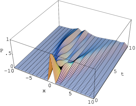
FIG. 1.: Time evolution of an unobserved particle with mass $m$ = 1 started at time $t_{0}$ = 0 from $x_{0}$ = 0 in the potential (19). Shown is the transition probability $p(x|\Delta t=t,x_{0}=1,v_{\rm true})$.

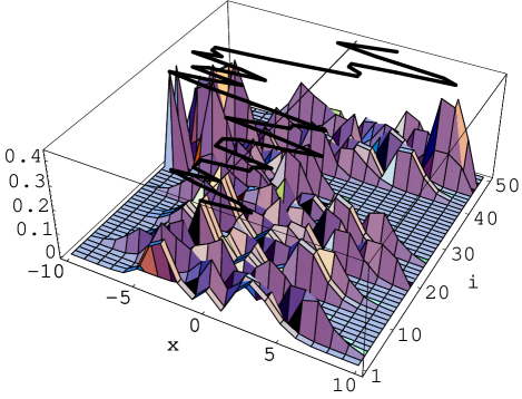
FIG. 2.: Time evolution of an observed particle with mass $m$ = 1 in the potential (19). The figure shows for each data point $i$ the probability $p(x|\Delta_{i}=5,x_{i-1},v_{\rm true})$, starting from $x_{0}$ = 0. (Hence, the probability at $i$ =1 corresponds to that shown in Fig. 1 at $t$ = 5.) The actual data points $x_{i}$ have been sampled from that probabilities and form the observed path shown on top as a thick line.

FIG. 3.: Numerical reconstruction of a potential from 50 coordinate measurements (see Fig. 2). Shown are the true potential $v_{\rm true}$ (thin line), the best parametric approximation used as reference potential $v_{0}$ (dashed line), and the reconstructed potential $v_{\rm ITDQ}$ (thick line). Parameters: $m$ = 1, $\Delta_{i}$ = 5, $v_{\rm true}$ of Eq. (19), $v_{0}$ of the form (21), Gaussian prior with ${\bf K}_{0}$ as in (20) with $\lambda$ = 0.1 and $\sigma_{0}$ = 3, $p_{E}$ (6) with $\mu$ = 10 and $\kappa$ = $E_{0}(v_{\rm true})$, periodic boundary conditions for $\psi_{\alpha}$, fixed boundary values $v(-10)$ = $v(10)$ = $10^{5}$ for $v_{\rm ITDQ}$, $v_{0}$ and $v_{\rm true}$, calculated on a lattice with 21 points. Errors: $\epsilon_{D}(v_{\rm ITDQ})$ = 99.1, $\epsilon_{D}(v_{\rm true})$ = 104.4, $\epsilon_{g}(v_{\rm ITDQ})$ = 1.891, $\epsilon_{g}(v_{\rm true})$ = 1.818.

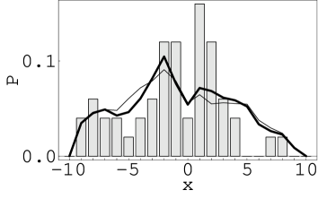
FIG. 4.: Sum of empirical transition probabilities $p_{\rm emp}$ (bars), the corresponding true $p_{\rm true}$ (thick line) for $v_{\rm true}$, and the reconstructed $p_{\rm ITDQ}$ (thin line).

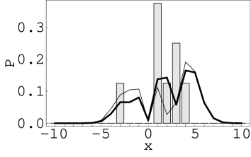
FIG. 5.: Same functions as in Fig. 4, but restricted to measurements of a particle which has been at position $x_{i-1}$ = 1 at the time of the previous measurement.

REFERENCES

- [1] K. Chadan and P. C. Sabatier, Inverse Problems in Quantum Scattering Theory (Springer Verlag, New York, 1989).
- [2] R. G. Newton, Inverse Schrödinger Scattering in Three Dimensions (Springer Verlag, Berlin, 1989).
- [3] J. M. Bernado and A. F. Smith, Bayesian Theory (Wiley, New York, 1994).
- [4] J. C. Lemm, J. Uhlig, and A. Weiguny, Technical Report No. MS-TP1-99-6, Univ. of Münster, arXiv:cond-mat/9907013 (accepted for publication by Phys. Rev. Lett.
- [5] J. C. Lemm and J. Uhlig, Technical Report No. MS-TP1-99-10, Univ. of Münster, arXiv:nucl-th/9908056.
- [6] G. Wahba, Spline Models for Observational Data (SIAM, Philadelphia, 1990).
- [7] C. K. I. Williams and C. E. Rasmussen, in NIPS 8, edited by D. S. Touretzky, M. C. Mozer, and M. E. Hasselmo (The MIT Press, Cambridge, MA, 1996), pp. 514–520.
- [8] C. K. I. Williams and D. Barber, IEEE Trans. on Pattern Analysis and Machine Intelligence 20, 1342 (1998).
- [9] J. C. Lemm, Technical Report No. MS-TP1-99-1, Univ. of Münster, arXiv:physics/9912005.
- [10] D. J. C. MacKay, in Maximum Entropy and Bayesian Methods, Santa Barbara 1993., edited by G. Heidbreder (Kluwer, Dordrecht, 1994).
- [11] B. Efron and R. J. Tibshirani, An Introduction to the Bootstrap (Chapman & Hall, New York, 1993).