Upper Bound on the region of Separable States near the Maximally Mixed State

Abstract

A lower bound on the amount of noise that must be added to a GHZ-like entangled state to make it separable (also called the random robustness) is found using the transposition condition. The bound is applicable to arbitrary numbers of subsystems, and dimensions of Hilbert space, and is shown to be exact for qubits. The new bound is compared to previous such bounds on this quantity, and found to be stronger in all cases. It implies that increasing the number of subsystems, rather than increasing their Hilbert space dimension is a more effective way of increasing entanglement. An explicit decomposition into an ensemble of separable states, when the state is not entangled,is given for the case of qubits.

I Introduction

A key distinguishing feature of quantum physics from classical physics is the prediction of a new kind of correlation between physical quantities, called entanglement. Quantum entanglement has been often been referred to as the inseparability of composite quantum systems. Such an entangled composite system is said to be inseparable because it cannot be prepared by manipulating each subsystem separately, using only measurements and operations local to one subsystem at a time. If a composite quantum mechanical state is specified by some density matrix, how can we tell if the system is entangled?

Much work has been done studying the particular case of two subsystems, with each in a two dimensional Hilbert space (qubits). There is a good understanding of the entanglement for such systems and in fact a criterion, the partial transposition condition of Peres[2], indicates whether the subsystems are entangled. This, however, is a necessary and sufficient condition only when there are two subsystems, one with Hilbert space dimension $2$, and the other of dimension $2$ or $3$, as was shown by the Horodeckis[3]. For more complex systems, it only determines whether the state contains distillable entanglement, however there are also some states with bound entanglement, which are lumped together with the separable states by this criterion.

Lewenstein et. al.[4] have used the Peres condition to consider two subsystems, but with each subsystem now in a $N>2$ dimensional Hilbert space. Życzkowski et. al.[5] have, among other results, shown that all the mixed states in a sufficiently small neighbourhood of the maximally mixed state are separable. They also gave a bound on the size of this neighbourhood for small composite systems. Vidal and Tarrach[6] gave a lower bound on the size of this neighbourhood for arbitrary composite states, of any number of subsystems. Schack and Caves[7] gave bounds for composite systems composed of many qubits ($N=2$).

It has been pointed out by Braunstein et. al.[8] that Maximally-entangled states of the GHZ type, with noise added, are connected to recent proposals for NMR quantum computing. They are also relevant to fundamental tests of quantum mechanics using Bell inequalities. The separability of such noisy generalised singlet states has been considered by various authors recently, mostly for the case of qubits (subsystems with Hilbert space dimension two). Schack and Caves[7], using the approach of Braunstein et. al. have obtained an exact boundary condition for the Werner states[9] (two qubits), while Caves and Milburn[10] extended the approach to two q-trits (Hilbert space dimension three). The Horodeckis[11] gave exact bounds for the case of two subsystems.

In this paper we extend the approach of Peres[2] to consider such noisy generalised singlet states in the general case of $D$ subsystems with each subsystem in a $N$ dimensional Hilbert space. A parameter $\epsilon$ specifies the amount of the pure GHZ-type maximally-entangled states present compared with the maximally-mixed noise state.We then ask and answer the following question: what is the maximum value of $\epsilon$ for this state to be entangled? Another fundamental question is also considered. To create as entangled a state as possible, is it simply better to increase the dimension of the subsystems or is it better to increase the number of subsystems?

II Generalised Werner states

The states considered here, consist of a mixture of the maximally-mixed noise states, and the GHZ-type entangled states, where the number $D$ of subsystems over which entanglement occurs, and the Hilbert space dimension $N$ of each subsystem (equal for all $D$ subsystems) can take on any values $N>1$, $D>1$. The relative proportion of GHZ-type states is controlled by the parameter $\varepsilon$, where $\varepsilon=1$ corresponds to a pure GHZ-type state, while $\varepsilon=0$ corresponds to the maximally mixed state. Explicitly, the state is given by the density operator

$$\hat{\rho}\>\> = (1-\varepsilon)\hat{\rho}_{n}+\varepsilon\hat{\rho}_{e},$$ (2)

$$\hat{\rho}_{n} = \frac{1}{N^{D}}\sum_{i_{1},i_{2},\dots,i_{D}=1}^{N}\left|{i_{1}i_{2}\dots i_{D}}\right\rangle\left\langle{i_{1}i_{2}\dots i_{D}}\right|,$$ (3)

$$\hat{\rho}_{e} = \frac{1}{N}\sum_{n,m=1}^{N}\left|{nn\dots n}\right\rangle\left\langle{mm\dots m}\right|,$$ (4)

where

$$\left|{i_{1}i_{2}\dots i_{D}}\right\rangle=\left|{i_{1}}\right\rangle\otimes\left|{i_{2}}\right\rangle\otimes\cdots\otimes\left|{i_{D}}\right\rangle.$$ (5)

Here $\left|{i_{k}}\right\rangle$ represents one of $N$ complete orthogonal basis states for the $k^{\rm th}$ subsystem, while $\hat{\rho}_{n}$ is the density operator for the maximally mixed state, and $\hat{\rho}_{e}$ for the GHZ-like state.

The Werner state[9], consisting of a singlet state and some noise, is the simplest $D=N=2$ case, hence we call these generalised Werner states. The state $\hat{\rho}$ can be viewed as a generalised singlet state $\hat{\rho}_{e}$ after it has emerged from a depolarising channel.

III Separability

The separability of particular cases of the state (II), and of more general states, has been considered previously by a number of authors [5, 6, 7, 8, 9, 10, 11, 12, 13]. Firstly, it was shown [12, 13] that for the two-qubit ($N=2,D=2$) case, (The Werner state) $\hat{\rho}$ is separable for $\varepsilon\leq 1/3$, and entangled otherwise, whereas for three qubits ($N=2,D=3$), Schack and Caves[7] found the state to be separable for $\varepsilon\leq 1/5$. Soon after, Horodecki and Horodecki[11] found the exact result for arbitrary numbers of qubits:

$$\varepsilon_{\text{separable}}\leq\frac{1}{1+N}.$$ (6)

Schack and Caves also found bounds on the size of the separable neighbourhood around the maximally mixed state for totally general states of many qubits ($N=2$). For $D=4$ and $D=5$ these are $\varepsilon\leq 1/33$ and $\varepsilon\leq 1/243$ respectively, and for higher $D$ are given by

$$\varepsilon_{\text{separable}}\leq\left\{\begin{array}[]{ll}1\ /\ (1+2^{D}+2^{2D-2})&{\rm{if\;D\;even}}\\ 1\ /\ (1-2^{D}+2^{2D-2})&{\rm{if\;D\;odd}}\end{array}\right.$$ (7)

What about the more general case when $N$ and $D$ are arbitrary? For what values of $\varepsilon$ is the state given by (II) separable? Vidal and Tarrach[6] gave a maximum bound for the random robustness $R$ of arbitrary multi-component states. For the states considered here, the critical value of $\varepsilon$ at which the states change from being entangled to separable is $\varepsilon_{c}=1/(1+R(\hat{\rho}_{e}||\hat{\rho}_{n}))$ (in the notation of ref.[6]). So according to that bound,

$$\varepsilon_{\text{entangled}}>\frac{1}{(1+N/2)^{D-1}}$$ (8)

We will prove in the next section (section IV) that the states given by (II), are always entangled if

$$\varepsilon_{\text{entangled}}>\frac{1}{N^{D-1}+1}.$$ (9)

That this bound is strong for qubits ($N=2$) is shown in appendix (A), and an explicit decomposition into product states is given for the case of separable $\hat{\rho}$.

IV Outline of the proof of (6)

Peres[2] has shown that a necessary condition for a state consisting of two subsystems to be separable is that the partial transpose of the density matrix over one of the subsystems, and the partial transpose over the other subsystem, have positive eigenvalues. However, this is a necessary and sufficient condition only when one of the subsystems has Hilbert space dimension $2$ or $3$, and the other dimension $2$, as was shown by the Horodeckis[3]. That paper went on to give a necessary and sufficient condition for a state to be separable. Nevertheless the Peres condition is just what is needed for an upper bound on $\varepsilon$ for separable states. i.e. any states which break the condition are entangled, although some which satisfy it may also be, but do not have to be, entangled. It is worth noting that any states which satisfy the Peres condition but are entangled are said to contain only “bound” entanglement, as it cannot be used for teleportation, nor distilled by the process of entanglement distillation.

Firstly, note that the Peres condition is easily extended to more than two entangled subsystems. If there are $D$ subsystems, one simply chooses some group of $M<D$ original subsystems to be called half-system number $1$, and the remaining subsystems to be called half-system number $2$. If for any such group of subsystems, an eigenvalue of the partial transpose of $\hat{\rho}$ over half-system number $1$ (say) is negative, then $\hat{\rho}$ is entangled. Thus to use the Peres condition to full advantage, one must consider all such groups of subsystems.

The state (II) is convenient in this respect, because it is unchanged under relabeling of the subsystems (evident by inspection). Thus the eigenvalues of $\rho^{T}_{\alpha}$, the partial transpose of $\hat{\rho}$ over the set $\alpha$ of subsystems, need only be looked at for $D/2$ (rounded down) sets of subsystems to extract the maximum benefit from the Peres condition. In particular, a choice of sets of subsystems can be $\alpha_{M}=\{1,2,\dots,M\}$ where $M=1,2,\dots,D/2$, and $\alpha_{M}$ contains the labels of the subsystems to be considered as members of the $M$th half-system.

Firstly let’s consider $M=1$, i.e. the first subsystem’s entanglement with the remaining $D-1$ of them. The partially transposed density matrix is

$$\rho^{T}_{1} = (1-\varepsilon){\rho}^{T}_{n}+\varepsilon{\rho}^{T}_{e},$$ (11)

$${\rho}^{T}_{n} = \frac{1}{N^{D}}\sum_{i_{1},i_{2},\dots,i_{D}=1}^{N}\left|{i_{1}i_{2}\dots i_{D}}\right\rangle\left\langle{i_{1}i_{2}\dots i_{D}}\right|,$$ (12)

$${\rho}^{T}_{e} = \frac{1}{N}\sum_{n,m=1}^{N}\left|{mn\dots n}\right\rangle\left\langle{nm\dots m}\right|.$$ (13)

Since all of the elements of $\hat{\rho}$, (hence $\rho^{T}_{1}$) are finite, the eigenvalues of $\rho^{T}_{1}$ must also be finite. Now, exploiting the general continuity property of eigenvalues of $\hat{\rho}_{1}^{T}$, we conclude that at the value of $\varepsilon=\varepsilon_{o}$ above which the Peres condition indicates the state is entangled, one or more eigenvalues of $\rho^{T}_{1}$ must be zero, since they are all positive for $\varepsilon<\varepsilon_{o}$, and at least one is negative for $\varepsilon>\varepsilon_{o}$. i.e. for some nonzero eigenvector

$$\left|{\psi}\right\rangle=\sum_{j_{1},j_{2},\dots,j_{D}=1}^{N}\psi_{j_{1}j_{2}\dots j_{D}}\left|{j_{1}j_{2}\cdots j_{D}}\right\rangle\neq 0$$ (14)

we must have $\rho^{T}_{1}(\varepsilon_{o})\left|{\psi}\right\rangle=0$. Expanded, this gives

$$\frac{1-\varepsilon_{o}}{N^{D}}\sum_{i_{1},i_{2},\dots,i_{D}=1}^{N} \psi_{i_{1}i_{2}\dots i_{D}} \left|{i_{1}i_{2}\cdots i_{D}}\right\rangle$$ (15)

$$+\frac{\varepsilon_{o}}{N}\sum_{n,m=1}^{N} \psi_{nm\dots m} \left|{mn\cdots n}\right\rangle=0.$$ (16)

Equation (15) can explicitly be written out as $N^{D}$ equations

$$(1-\varepsilon_{o}) \psi_{i_{1}i_{2}\dots i_{D}}$$ (17)

$$+ \varepsilon_{o}N^{D-1}\delta_{i_{2}i_{3}}\delta_{i_{2}i_{4}}\cdots\delta_{i_{2}i_{D}}\psi_{i_{2}i_{1}\dots i_{1}}=0,$$ (18)

where $\delta_{ab}=1$ if $a=b$, $0$ otherwise. Now if one or more of the $i_{a}:a=3,\dots,D$ does not equal $i_{2}$, then that equation is satisfied only if $\varepsilon=1$ or $\psi_{i_{1}i_{2}\dots i_{D}}=0$. The first case is not of interest here, as $\varepsilon=1$ corresponds to our maximally entangled GHZ like states, so we choose $\psi_{i_{1},i_{2}\dots i_{D}}=0$.

The rest of the equations where $i_{2}=i_{3}=\cdots=i_{D}$, separate into $N(N-1)/2$ coupled sets of two equations of the identical form

$$(1-\varepsilon_{o})\psi_{ab\dots b}+\varepsilon_{o}N^{D-1}\psi_{ba\dots a} = 0,$$ (19)

$$(1-\varepsilon_{o})\psi_{ba\dots a}+\varepsilon_{o}N^{D-1}\psi_{ab\dots b} = 0.$$ (20)

These have solutions if $\psi_{ab\dots b}=\psi_{ba\dots a}=0$, but this would imply $\left|{\phi}\right\rangle=0$, which was specifically excluded in (14). Otherwise, these coupled two equations are only satisfied if

$$\varepsilon_{o}=\frac{1}{N^{D-1}+1}.$$ (21)

So for $\left|{\psi}\right\rangle\neq 0$, at least one such coupled set of two equations leads to the expression (21). This is the only candidate for the point where the Peres condition becomes satisfied.

Now it can be easily seen that in the total-noise case $\varepsilon=0$, $\rho^{T}_{1}=\hat{\rho}$ and all the eigenvalues of $\rho^{T}_{1}$ are $1/(N^{D})$. In the no-noise case ($\varepsilon=1$), proceeding in similar fashion to before, the eigenvalues $\lambda$ of $\rho^{T}_{1}$ must satisfy

$$\frac{1}{N}\sum_{n,m=1}^{N} \psi_{nm\dots m} \left|{mn\cdots n}\right\rangle$$ (22)

$$= \lambda \sum_{i_{1},i_{2},\dots,i_{D}=1}^{N}\psi_{i_{1}i_{2}\dots i_{D}}\left|{i_{1}i_{2}\cdots i_{D}}\right\rangle.$$ (23)

This gives $\psi_{i_{1}i_{2}\dots i_{D}}=0$ if for some $a=3,4,\dots,D$, $i_{2}\neq i_{a}$, and leads to sets of two coupled equations of the form

$$\psi_{ab\dots b} = \lambda N\psi_{ba\dots a},$$ (24)

$$\psi_{ba\dots a} = \lambda N\psi_{ab\dots b}.$$ (25)

These have the solutions $\psi_{ab\dots b}=\psi_{ba\dots a}=0$ or

$$\lambda=\pm\frac{1}{N^{2}}.$$ (26)

As before, for nonzero eigenvectors, the first cannot be true. So, finally, for the no-noise state, at least one eigenvalue of $\rho^{T}_{1}$ must be negative, and equal to

$$\lambda=-\frac{1}{N^{2}}.$$ (27)

Thus, finally, since $\varepsilon_{o}$ is the only value of $\varepsilon$ where an eigenvalue of $\rho^{T}_{1}$ is zero, all eigenvalues are positive for $\varepsilon=0$, and an eigenvalue is negative for $\varepsilon=1$, there must be at least one negative eigenvalue for $\varepsilon>\varepsilon_{o}$ given by (21).

When one proceeds in the same fashion when $M=2,3,\dots,D/2$, one always gets coupled sets of two equations identical in form to (19), as can be seen by inspection, so nothing new is found. Thus the result of section (II) is indicated.

V Comparison to known bounds

For the qubit case ($N=2$), as seen in figure (1), equation (9) gives an exact bound on the values of $\varepsilon$ that divide separable from entangled states of the form (II). One sees that the upper bound (8) derived from the work of Vidal and Tarrach comes very close to the exact value for the qubit case. This exact bound is also greater than those lower bounds previously found by Schack and Caves[7], as expected.

For the two-subsystem ($D=2$) case, the bound (9) agrees with the exact one found by the Horodeckis[11].

For other values of $D$ and $N$, the results on random robustness by Vidal and Tarrach, lead to an upper bound which is considerably weaker than the upper bound (9) given by the partial transposition condition. The upper bound found here, actually gives a stronger bound on the random robustness of entanglement of states given by (II).

$$R(\hat{\rho}_{e}||\hat{\rho}_{n})\leq N^{D-1}$$ (28)

It is interesting to note that in the border cases when $N=2$ or $D=2$, the bound (9) is in fact an exact bound. This is despite the fact that the Peres condition does not necessarily give a strong bound for such states. This leads one to the tentative conjecture that for noisy GHZ-type states of the form (II), the Peres condition may in general give a strong upper bound.

Looking at figure (2), one sees that as the Hilbert space dimension of the subsystems increases, the upper bound on $\varepsilon$ rapidly decreases, indicating that the entanglement becomes stronger.

As the bound (9) is completely general in $N$ and $D$, it does provide some answers to the question of what raises entanglement more: creating more entangled subsystems, or increasing their dimension? Since the bound on $\varepsilon$ decreases exponentially with $D$, but only polynomially with $N$, one concludes that increasing the number of subsystems is a more effective way of increasing the entanglement.

VI Conclusion

The results presented here based on the Peres condition provide a lower bound on the parameters $\varepsilon$ in (II) above which the generalised Werner states are always entangled. Furthermore, it gives an exact bound on this parameter for the case of many qubits. An explicit simple expression is derived that depends on $D$, the number of subsystems over which entanglement occurs, and $N$ the Hilbert space dimension of each subsystem. Apart from the few cases ($D=2$;$N=2$ and $D=3$) where this bound was known exactly previously, the new bounds are stronger than previously known ones.

This work also sheds light on the question of whether to increase quantum entanglement in a system, is it better to create more entangled subsystems, or to increase the dimension of the existing subsystem. As the bound on $\varepsilon$ decreases exponentially with $N$, but only polynomially with $D$, increasing the number of subsystems is a much more effective way of increasing entanglement.

To conclude, the Peres partial transposition condition has provided a good upper bound for determining the separability of a generalised $N$, $D$ Werner state. However for other systems it is known that this transposition condition fails to give strong results, thus when this condition is useful, and when not, remains an interesting question.

A Proof that (6) is exact for qubits

We wish to show that the bound (9) is exact for qubits ($N=2$), and to find the product states which combine to give the state when it is separable.

Starting off similarly to Schack and Caves[7], the $D$-subsystem generalisation of the Werner state ((II) with $N=2$) can be written in terms of Pauli matrices:

$$\hat{\rho}(\varepsilon)=\frac{1}{2^{D}}\left\{(1-\varepsilon)I^{\otimes D}+\frac{\varepsilon}{2}\hat{E}\right\},$$ (A2)

where

$$\hat{E}= (I+\sigma_{3})^{\otimes D}+(I-\sigma_{3})^{\otimes D}$$ (A3)

$$+(\sigma_{1}+i\sigma_{2})^{\otimes D}+(\sigma_{1}-i\sigma_{2})^{\otimes D},$$ (A4)

and $\sigma_{i}$ are the Pauli matrices, $I$ is the two-dimensional identity matrix, and for conciseness, the following notation is used:

$$(A)^{\otimes D}=(A)\otimes\cdots\otimes(A)\qquad\text{{\hbox{D}} times}.$$ (A5)

To show that (9) is actually a strong bound, is suffices to find an expansion of $\rho$ in terms of a positive sum of direct tensor products of density matrices for this value of

$$\varepsilon=\varepsilon_{c}=\frac{1}{2^{D-1}+1}.$$ (A6)

By analogy with the results of Schack and Caves [7], it has been guessed that an expansion of $\rho(\varepsilon_{c})$ in terms of the density matrices

$$P_{\pm i}=\frac{1}{2}(I\pm\sigma_{i})\qquad\text{ ({\hbox{i = 1,2,3}})},$$ (A7)

is given by the following:

$$\hat{\rho}_{g}=\frac{\varepsilon_{c}}{2}\left(P_{3}^{\otimes D}+P_{-3}^{\otimes D}\right)+\frac{\varepsilon_{c}}{2^{D-1}}\sum P_{x_{1}}\otimes P_{x_{2}}\otimes\cdots\otimes P_{x_{D}}.$$ (A8)

Here the sum is over all permutations of $D$ indices $x_{1},x_{2},\dots,x_{D}$ satisfying the following conditions:

1. $x_{i}\in\{1,-1,2,-2\}$.

2. The number of $x_{i}\in\{2,-2\}$ is even (or zero).

3. If the number of $x_{i}\in\{2,-2\}$ is a multiple of four (or is zero), then the number of $x_{i}\in\{-1,-2\}$ is even (or zero).

4. If the number of $x_{i}\in\{2,-2\}$ is not a multiple of four, then the number of $x_{i}\in\{-1,-2\}$ is odd.

The proof of this proceeds by starting with the above guess, and showing that it is a correct one. As it turns out, the hard work is in actually writing down the guess mathematically, so let us begin with this.

To begin with, note that

$${\cal T}_{0} = (P_{1}+P_{2}+P_{-1}+P_{-2})^{\otimes D}$$ (A9)

$$= \sum P_{x_{1}}\otimes P_{x_{2}}\otimes\cdots\otimes P_{x_{D}},$$ (A10)

where the sum is over all permutations of $D$ indices $x_{1},x_{2},\dots,x_{N}\in\{1,2,-1,-2\}$. Also note that

$${\cal S}_{0}=(P_{1}+P_{2}-P_{-1}-P_{-2})^{\otimes D}$$ (A11)

will give a sum over all these permutations, except that all terms which have an odd number of indices in $\{-1,-2\}$ will be subtracted rather than added like in ${\cal T}_{0}$. Thus one can see that

$${\cal R}_{0}^{e}=\frac{1}{2}[{\cal T}_{0}+{\cal S}_{0}]$$ (A13)

will give a sum over permutations of $D$ indices, like ${\cal T}_{0}$, except that only terms where the number of indices in $\{-1,-2\}$ is even will be included. Similarly

$${\cal R}_{0}^{o}=\frac{1}{2}[{\cal T}_{0}-{\cal S}_{0}]$$ (A14)

will give a sum over only those terms in which the number of indices in $\{-1,-2\}$ is odd.

Now consider some more similar expressions.

$${\cal T}_{1}=(P_{1}-P_{2}+P_{-1}-P_{-2})^{\otimes D}.$$ (A15)

${\cal T}_{1}$ will give a sum over all index permutations, except that all terms which have an odd number of indices in $\{2,-2\}$ will be subtracted rather than added like for ${\cal T}_{0}$.

$${\cal T}_{2}=(P_{1}+iP_{2}+P_{-1}+iP_{-2})^{\otimes D}.$$ (A16)

${\cal T}_{2}$ will give a similar sum over all permutations, but terms in which the number of indices in $\{2,-2\}$ is a multiple of four (or is zero) will be added, terms in which this number is even, but not a multiple of four, will be subtracted, terms in which this number is one more than a multiple of four will be added and multiplied by $i$, and terms for which this number is one less than a multiple of four will be subtracted and multiplied by $i$.

$${\cal T}_{3}=(P_{1}-iP_{2}+P_{-1}-iP_{-2})^{\otimes D}.$$ (A17)

${\cal T}_{3}$ is the complex conjugate of ${\cal T}_{2}$. It can be seen (after a little thought) that $\frac{1}{4}[{\cal T}_{0}+{\cal T}_{1}+{\cal T}_{2}+{\cal T}_{3}]$ will give a sum over only those terms in which the number of indices in $\{2,-2\}$ is a multiple of four (or is zero). Similarly, $\frac{1}{4}[{\cal T}_{0}+{\cal T}_{1}-{\cal T}_{2}-{\cal T}_{3}]$ will give a sum over only those terms in which the number of indices in $\{2,-2\}$ is even, but not a multiple of four.

Analogously to equation (A11) define

$${\cal S}_{1}=(P_{1}-P_{2}-P_{-1}+P_{-2})^{\otimes D},$$ (A19)

$${\cal S}_{2}=(P_{1}+iP_{2}-P_{-1}-iP_{-2})^{\otimes D},$$ (A20)

$${\cal S}_{3}=(P_{1}-iP_{2}-P_{-1}+iP_{-2})^{\otimes D},$$ (A21)

and one can define expressions for ${\cal R}_{i}^{e}$ and ${\cal R}_{i}^{o}$ for $i=0,1,2,3$ analogously to equations (A11). So following the same reasoning as previously, the sum of all terms in which the number of indices in $\{2,-2\}$ is a multiple of four, and the number of indices in $\{-1,-2\}$ is even is given by

$$\frac{1}{4}[{\cal R}_{0}^{e}+{\cal R}_{1}^{e}+{\cal R}_{2}^{e}+{\cal R}_{3}^{e}].$$ (A22)

And thus finally, the sum in the second term of the guess $\rho_{g}$ ( equation (A8) ) can be written

$$\frac{1}{4}[{\cal R}_{0}^{e}+{\cal R}_{1}^{e}+{\cal R}_{2}^{e}+{\cal R}_{3}^{e}]+\frac{1}{4}[{\cal R}_{0}^{o}+{\cal R}_{1}^{o}-{\cal R}_{2}^{o}-{\cal R}_{3}^{o}]$$ (A23)

$$=\frac{1}{4}[{\cal T}_{0}+{\cal T}_{1}+{\cal S}_{2}+{\cal S}_{3}].$$ (A24)

So the guess that has been made (i.e. equation (A8)) can be rewritten

$$\rho_{g}=\frac{\varepsilon_{c}}{2}\left(P_{3}^{\otimes N}+P_{-3}^{\otimes N}\right)+\frac{\varepsilon_{c}}{2^{N+1}}\left[{\cal T}_{0}+{\cal T}_{1}+{\cal S}_{2}+{\cal S}_{3}\right],$$ (A25)

which is explicitly (via the expressions (A9), (A11), (A15), (A)) a positive sum of direct tensor products of density matrices, and thus is separable. The only question that remains is whether $\rho_{g}=\rho(\varepsilon_{c})$ ?

This is the easy part. It is seen using the expression (A7) that

$${\cal T}_{0} = (2I)^{\otimes N}=2^{N}I^{\otimes N},$$ (A27)

$${\cal T}_{1} = 0,$$ (A28)

$${\cal S}_{2} = (\sigma_{1}+i\sigma_{2})^{\otimes N},$$ (A29)

$${\cal S}_{3} = (\sigma_{1}-i\sigma_{2})^{\otimes N},$$ (A30)

$$P_{3}^{\otimes N} = 2^{-N}(I+\sigma_{3})^{\otimes N},$$ (A31)

$$P_{-3}^{\otimes N} = 2^{-N}(I-\sigma_{3})^{\otimes N},$$ (A32)

so

$$\rho_{g}=\frac{\varepsilon_{c}}{2}I^{\otimes N}+\frac{\varepsilon_{c}}{2^{N+1}}\hat{E},$$ (A33)

which only seemingly differs from equation (A) by the first term, but using the expression for $\varepsilon_{c}$ (A6), one finds that these first terms are equal also.

$$\frac{1-\varepsilon_{c}}{2^{N}}=\frac{\varepsilon_{c}}{2},$$ (A34)

so $\rho_{g}=\rho$, the guess was correct, and thus the bound $\varepsilon_{c}$ is strong.

${\cal QED}$

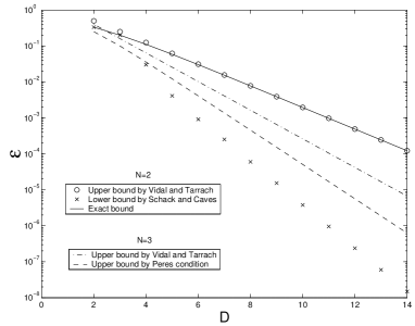
FIG. 1.: Bounds on the value of $\varepsilon$ for which the states (II) become separable or entangled, for the qubit ($N=2$) and q-trit ($N=3$) cases, shown on the same plot. When $\varepsilon$ is above the upper bounds or the exact bound, $\hat{\rho}$ is entangled, and when $\varepsilon$ is below the lower bound or the exact bound, $\hat{\rho}$ is always separable. When $\varepsilon$ is below an upper bound, $\hat{\rho}$ may be separable or bound entangled.

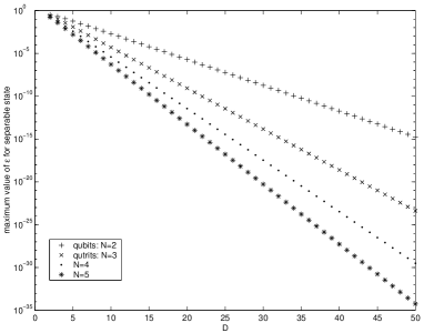
FIG. 2.: Upper bounds on $\varepsilon$ for separable states of the form (II) on a logarithmic scale. Variation with subsystem Hilbert-space dimension $N$ is shown.

REFERENCES

• [1] Email address: deuar@physics.uq.edu.au
• [2] A. Peres, Phys. Rev. Lett. 77, 1413 (1996).
• [3] M. Horodecki, P. Horodecki, and R. Horodecki, Phys. Lett. A 223, 1 (1996); (quant-ph/9605038).
• [4] M. Lewenstein, J. I. Cirac, and S. Karnas, quant-ph/9903012 (1999).
• [5] K. ลปyczkowski, P. Horodecki, A. Sanpera, and M. Lewenstein, Phys. Rev. A 58, 883 (1998).
• [6] G. Vidal and R. Tarrach, Phys. Rev. A 59, 141 (1999).
• [7] R. Schack and C. M. Caves (quant-ph/9904109) (1999).
• [8] S. L. Braunstein, C. M. Caves, R. Jozsa, N. Linden, S. Popescu, and R. Schack, Phys. Rev. Lett. 83, 1054 (1999).
• [9] R. F. Werner, Phys. Rev. A 40, 4277 (1989).
• [10] C. M. Caves and G. J. Milburn, to be published (1999).
• [11] M. Horodecki and P. Horodecki, Phys. Rev. A 59, 4206 (1999).
• [12] M. Murao, M. B. Plenio, S. Popescu, V. Vedral, and P. L. Knight, Phys. Rev. A 57, R4075 (1998).
• [13] R. Horodecki and M. Horodecki, Phys. Rev. A 54, 1838 (1996).
Refer to caption
FIG.โ€„1.: Bounds on the value of $\varepsilon$ for which the states (II) become separable or entangled, for the qubit ($N=2$) and q-trit ($N=3$) cases, shown on the same plot. When $\varepsilon$ is above the upper bounds or the exact bound, $\hat{\rho}$ is entangled, and when $\varepsilon$ is below the lower bound or the exact bound, $\hat{\rho}$ is always separable. When $\varepsilon$ is below an upper bound, $\hat{\rho}$ may be separable or bound entangled.
Refer to caption
FIG.โ€„2.: Upper bounds on $\varepsilon$ for separable states of the form (II) on a logarithmic scale. Variation with subsystem Hilbert-space dimension $N$ is shown.