Optimal States for Bell inequality Violations using Quadrature Phase Homodyne Measurements

Abstract

We identify what ideal correlated photon number states are to required to maximize the discrepancy between local realism and quantum mechanics when a quadrature homodyne phase measurement is used. Various Bell inequality tests are considered.

I Introduction

There has been recently active interest in tests of quantum mechanics[1] versus local realism in a high efficiency detection limit. Several authors[2, 3, 4] including ourselves have considered detection schemes quadrature phase homodyne measurements. Such schemes use strong local oscillators and hence have very high detection efficiency[5]. This removes one of the current loopholes[6, 7, 8, 9] and potentially allows a strong test of quantum mechanics[10] to be performed.

The original idea of Gilchrist et. al.[2] was to use a circle or pair coherent state[11, 12, 13] produced by nondegenerate parametric oscillation with the pump mode adiabatically eliminated. Using highly efficient quadrature phase homodyne measurements, the Clauser Horne strong Bell inequality[14, 15, 16] could be tested in an all optical regime. A small (approximately $1.5\%$) but significant theoretical violation was found for this extremely idea system. While the mean photon number for the system may be low (approximately $1.12$), the use of homodyne measurements allow a macroscopic current to be detected.

In this article, we take an unphysical but interesting approach and answer the following questions:

• Given that your detection scheme is a quadrature phase homodyne measurement, what is the optimal input or correlated photon number state to maximize the potential violation?

• What is the optimal Bell inequality to test?

To begin we will restrict our attention to correlated photon number states of the form

$$|\Psi\rangle=\sum_{n=0}^{\infty}c_{n}|n\rangle|n\rangle$$ (1)

Two main sources of correlated photon number currently exist, each having it own particular form of $c_{n}$. The most well known is simply the nondegenerate parametric amplifier specified by an ideal Hamiltonian of the form[17]

$$H=-\hbar\chi\epsilon\left(ab+a^{\dagger}b^{\dagger}\right).$$ (2)

where $\epsilon$ is field amplitude of a nondepleting classical pump and $\chi$ is proportional to the susceptibility of the medium. $a,b$ are the boson operators for the orthogonal signal and idler modes. After a time $\tau$, the state of the system is given by (1) with $c_{n}$ specified by

$$c_{n}={{\tanh^{n}\left[\chi\epsilon\tau\right]}\over{\cosh\left[\chi\epsilon\tau\right]}}$$ (3)

In the quadrature phase amplitude basis this state has a positive Wigner function. Hence it can be described as a local hidden variable theory and thus cannot violate a Bell inequality.

The other source of highly correlated photon number states exists in nondegenerate parametric oscillation. In the limit of very large parametric nonlinearity and high Q cavities, a state of the form[13]

$$|\Psi\rangle={e^{r^{2}}\over\sqrt{4\pi^{2}I_{0}\left(2r^{2}\right)}}\int_{0}^{2\pi}d\theta\;|re^{i\theta}\rangle|re^{-i\theta}\rangle$$ (4)

can be generated. Here $r$ is the size of the circle of the coherent states and $I_{0}$ is the zeroth order modified Bessel function. Equivalently this state can be written in the form of (1) with $c_{n}$ given by

$$c_{n}={{r^{2n}}\over{n!I_{0}\left(2r^{2}\right)}}$$ (5)

This was the state considered by Gilchrist et. al.[2]

Given the general form of known correlated number states (1), the next fundamental question that should be initially addressed is what we mean by the Bell inequality. A number of Bell inequalities exist, and the particular one depends used heavy on your application and experimental setup. The Bell inequalities to be considered in this article are the Clauser Horne[15], the spin[14], and the information-theoretic[18] Bell inequality. A detailed derivation of the various inequalities will not be given, the reader is referred to references [15, 14, 18]. Here we will consider only strong inequalities, that is inequalities where auxiliary assumptions (not based on local realism) are not required. In Fig (1) we depict a very idealized setup for general Bell inequality experiment.

Probably the most well known inequality is the Clauser Horne strong Bell inequality[15] given by

$$|{\bf B}_{ch}|\leq 1$$ (6)

where

$$B_{ch}={{P_{11}\left(\theta,\phi\right)-P_{11}\left(\theta^{\prime},\phi\right)+P_{11}\left(\theta,\phi^{\prime}\right)+P_{11}\left(\theta^{\prime},\phi^{\prime}\right)}\over{P_{1}\left(\theta^{\prime}\right)+P_{1}\left(\phi\right)}}$$ (7)

Here $P_{11}$ is the probability that a “1” results occurs at each analyzer $A,B$ given $\theta,\phi$. Similarly $P_{1}$ is the probability that a “1” occurs at a detector while having no information about the second. For many of the actual experimental considerations an angle factorization occurs so that $P_{11}\left(\theta,\phi\right)$ depends only on $\theta+\phi$. Also $P_{1}\left(\theta\right)$ and $P_{1}\left(\phi\right)$ are independent of $\theta,\phi$. In this case $B_{ch}$ can be simplified to

$$B_{ch}={{3P_{11}\left(\psi\right)-P_{11}\left(3\psi\right)}\over{2P_{1}}}$$ (8)

where $\psi=\theta+\phi=-\theta^{\prime}-\phi^{\prime}=\theta+\phi^{\prime}$ and $3\psi=\theta^{\prime}+\phi$.

The second form of the Bell inequality (sometimes referred to as the spin or original Bell inequality) is[14]

$$B_{s}=|E\left(\theta,\phi\right) - E\left(\theta^{\prime},\phi\right)$$ (9)

$$+ E\left(\theta,\phi^{\prime}\right)+E\left(\theta^{\prime},\phi^{\prime}\right)|\leq 2$$ (10)

where the correlation function $E\left(\theta,\phi\right)$ is given by

$$E\left(\theta,\phi\right)=P_{11}\left(\theta,\phi\right) + P_{00}\left(\theta,\phi\right)$$ (11)

$$- P_{10}\left(\theta,\phi\right)-P_{01}\left(\theta,\phi\right)$$ (12)

Here as discussed above $P_{11}$ is probability that a “1” results occurs at each analyzer $A,B$ given $\theta,\phi$. $P_{00}$ is probability that a “0” results occurs at each analyzer $A,B$, while $P_{10}$ ($P_{01}$) is probability that a “1” (“0”) results occurs at the analyzer $A$ and a “0” (“1”) at $B$. With the angle factorization given above, the inequality (9) can be rewritten as

$$B_{s}=\left|3E\left(\psi\right)-E\left(3\psi\right)\right|\leq 2$$ (13)

Our final form of Bell inequality to be considered in this article was developed by Braunstein and Caves[18]. This classical information-theoretic Bell inequality has the form

$$B_{info}\geq 0$$ (14)

where

$$B_{info}=-H\left(\theta|\phi\right) + H\left(\theta|\phi^{\prime}\right)$$ (15)

$$+ H\left(\phi^{\prime}|\theta^{\prime}\right)+H\left(\theta^{\prime}|\phi\right)$$ (16)

Here $H\left(\theta|\phi\right)$ is given by

$$H\left(\theta|\phi\right)=-\sum_{a,b}P(a,b)\log\left({{P(a,b)}\over{P(a)}}\right)$$ (17)

with $\log\left(P(a,b)/P(a)\right)$ being the information gained at $B$ given the result at $A$ is known. The conditional information is then given by $H\left(\theta|\phi\right)$. The base of the logarithm determines the units of the information (base 2 for bits, base e for nats). For quantum computing purposes, this inequality should prove highly useful as it directly deals with information content. Several other Bell inequality do exist such as the CHSH inequality[6], but these are not considered here due to there weaker nature. Auxiliary assumptions are necessary in there derivation which open up several loopholes[7, 8, 9].

II Correlated States

From (1) we need to find the optimal $c_{n}$ which gives the largest Bell inequality violation. Before determining the $c_{n}$ we need to briefly focus our attention on the quadrature phase homodyne measurement.

A quadrature phase-amplitude homodyne measurement $X(\theta)$ at $A$ can achieved by combining a signal field (say $\hat{a}$) with a strong local oscillator field (say $\epsilon$) to form two new fields given by $\hat{c}_{\pm}=\left[\hat{a}\pm\epsilon\exp\left(i\theta\right)\right]/\sqrt{2}$. Here $\theta$ is a phase shift which allows the choice of particular observable to be measured, for instance choosing $\theta$ as $0$ or $\pi/2$ allows the measurement of the conjugate phase variables $X(0)$ and $X(\pi/2)$ respectively. The homodyne measurement gives the photocurrent difference as

$$I_{d} = c_{+}^{\dagger}c_{+}-c_{-}^{\dagger}c_{-}$$ (18)

$$= \epsilon\left(\hat{a}e^{-i\theta}+\hat{a}^{\dagger}e^{-i\theta}\right)=\epsilon X(\theta)$$ (19)

Performing a measurement on the quadrature phase amplitude $X(\theta)$ at $A$ yields a result $x_{1}(\theta)$ which ranges in size and sign. Similarly a measurement on the quadrature phase amplitude $X(\phi)$ at $B$ yields a result $x_{2}(\phi)$. For our state given by (1), the probability of obtaining the result $x_{1}(\theta),x_{2}(\phi)$ is simply

$$P_{x_{1}x_{2}}\left(\theta,\phi\right)=\left|\langle x_{1}(\theta)|\langle x_{2}(\phi)|\Psi\rangle\right|^{2}$$ (20)

where

$$\langle x(\varphi)|n\rangle={1\over{\sqrt{2^{n}n!\sqrt{\pi}}}}e^{-in\varphi}e^{-x_{i}^{2}/2}H_{n}(x_{i}).$$ (21)

Here $H_{n}(x_{i})$ is the Hermite polynomial and $\varphi$ is the phase of the local oscillator. Eqn (20) can be explicitly written as

$$P_{x_{1}x_{2}}\left(\psi\right) = \sum_{n,m}{{c_{n}c_{m}^{\ast}e^{-i(n-m)\psi}}\over{2^{n+m}n!m!\pi}}$$ (22)

$$\;\;\;\;\;\;\;\times\prod_{i=1}^{2}e^{-x_{i}^{2}}H_{n}(x_{i})H_{m}(x_{i})$$ (23)

where $\psi=\theta+\phi$, that is our expression depends only on the sum of the individual local angles.

The probability given by (22) is for continuous variables. The majority of the tests of quantum mechanics versus local realism require a binary result. Hence for a given quadrature measurement $x_{i}$ we classify the result as “1” if $x_{i}\geq 0$ and the mutually exclusive “0” if $x_{i}<0$. Here we have set the binning window about $x_{i}=0$. Where this binning window is located is quite arbitrary, but the maximum violation occurs for the value we have selected.

The probability of obtaining both particles in the “1” bin is

$$P_{11}\left(\psi\right) = \int_{0}^{\infty}\int_{0}^{\infty}dx_{1}dx_{2}P_{x_{1}x_{2}}\left(\psi\right)$$ (24)

while the probability of obtaining both particles in the “0” bin is

$$P_{00}\left(\psi\right) = \int_{-\infty}^{0}\int_{-\infty}^{0}dx_{1}dx_{2}P_{x_{1}x_{2}}\left(\psi\right)$$ (25)

The other probabilities such $P_{10}\left(\psi\right),P_{01}\left(\psi\right)$ can be calculated in a similar fashion. The probabilities formulated above are joint probabilities. Various of the strong Bell inequalities also require marginal probabilities of the form

$$P_{1}\left(\psi\right) = \int_{0}^{\infty}\int_{-\infty}^{\infty}dx_{1}dx_{2}P_{x_{1}x_{2}}\left(\psi\right)$$ (26)

The above integrals can be easy evaluated using the results[19]

$$\int_{0}^{\infty}e^{-x^{2}}H_{n}(x)H_{m}(x) = {{\pi 2^{n+m}}\over{n-m}}\left[{\cal F}(n,m)-{\cal F}(m,n)\right]$$ (27)

$$\;\;\;\;\;\;\;\;\;\;\;\;\;\;\;\;(for\;n\neq m)$$ (28)

$$\int_{-\infty}^{\infty}e^{-x^{2}}H_{n}(x)H_{m}(x) = 2^{n}n!\sqrt{\pi}\delta_{n,m}$$ (29)

where ${\cal F}(n,m)$ is given by

$${\cal F}^{-1}(n,m)=\Gamma\left({1\over 2}-{1\over 2}n\right)\Gamma\left(-{1\over 2}m\right)$$ (30)

with $\Gamma$ being the Gamma function. Performing the integrals for (24) and (25) we find

$$P_{11}\left(\psi\right) = P_{00}\left(\psi\right)$$ (31)

$$= {1\over 4}+\sum_{n>m}{{2^{n+m+1}\pi c_{n}c_{m}^{\ast}}\over{n!m!(n-m)^{2}}}$$ (32)

$$\;\;\;\times\left[{\cal F}(n,m)-{\cal F}(m,n)\right]^{2}\cos\left[(n-m)\psi\right]$$ (33)

Similarly Eqn (26) simplifies to

$$P_{1} = 1/2$$ (34)

which is independent of the sum of the local oscillator angle $\psi$. It is also simple to calculate the correlation function $E(\psi)$

$$E(\psi) = \sum_{n>m}{{2^{n+m+3}\pi c_{n}c_{m}^{\ast}}\over{n!m!(n-m)^{2}}}\left[{\cal F}(n,m)-{\cal F}(m,n)\right]^{2}$$ (35)

$$\;\;\;\;\;\;\;\;\;\times\cos\left[(n-m)\psi\right]$$ (36)

Given the probabilities $P_{11}$, $P_{00}$, $\ldots$ it is also possible to calculate the conditional information $H\left(\theta|\phi\right)$

$$H\left(\theta|\phi\right)= - P_{11}\log\left[2P_{11}\right]-P_{00}\log\left[2P_{00}\right]$$ (37)

$$- P_{10}\log\left[2P_{10}\right]-P_{01}\log\left[2P_{01}\right]$$ (38)

It is now possible to calculate the Clauser Horne (6) and spin (9) and information-theoretic (14) Bell inequalities. Some insight into the problem can be achieved by a careful examination of the term

$${{2^{n+m}\pi}\over{n!m!(n-m)^{2}}}\left[{\cal F}(n,m)-{\cal F}(m,n)\right]^{2}$$ (39)

which is present in all the joint probability distributions. This expression has several interesting features. First, as the difference between $n$ and $m$ becomes large, the smaller that the above expression contributes to any of the probability distributions. The main contribution for the expression comes from the case $m=n\pm 1$. Second, when $n-m$ is even, the above expression is zero. Finally, as $n$ is large the different between the $n,m=n-1$ and $n+1,m=n$ elements for fixed large $n$ vanishes and they reach an asymptotic limit which is smaller than the $n=1,m=0$ case. If these higher order $n$ terms dominate due to the choice of the $c_{n}$ in the probability formula, then the various Bell inequalities can not violated. This also has the implication that the mean photon number cannot be high if a violation is to occur and hence it is not a macroscopic test of quantum mechanics.

III A simple Case

To begin our investigations of the Bell inequalities, consider the case of we have only two photon pair states that is,

$$|\Psi\rangle=c_{0}|0\rangle|0\rangle+c_{1}|1\rangle|1\rangle$$ (40)

where for convenience we choose $c_{n}$ real. We also require $c_{0}^{2}+c_{1}^{2}=1$. The joint probability distributions are readily calculated and in fact

$$P_{11}\left(\psi\right)=P_{00}\left(\psi\right) = {1\over 4}+{{c_{0}c_{1}}\over{\pi}}\cos\left[\psi\right]$$ (41)

$$P_{10}\left(\psi\right)=P_{01}\left(\psi\right) = {1\over 4}-{{c_{0}c_{1}}\over{\pi}}\cos\left[\psi\right]$$ (42)

Calculating $B_{ch}$ and $B_{s}$ from (6) and (9) we find

$$B_{ch} = {1\over 2}+{{c_{0}c_{1}}\over{\pi}}\left\{3\cos\left[\psi_{0}\right]-\cos\left[3\psi\right]\right\}$$ (44)

$$B_{s} = {{4c_{0}c_{1}}\over{\pi}}\left\{3\cos\left[\psi_{0}\right]-\cos\left[3\psi\right]\right\}$$ (45)

Optimizing for the angle $\psi$ we find

$$B_{ch} = {1\over 2}+{{2\sqrt{2}c_{0}c_{1}}\over{\pi}}$$ (47)

$$B_{s} = {{8\sqrt{2}c_{0}c_{1}}\over{\pi}}$$ (48)

that is, $|B_{ch}|\leq 1$ and $|B_{s}|\leq 2$ for all $c_{0}$. No violation of the strong Clauser Horne or spin Bell inequality is possible.

For the information theoretic case we find

$$H\left(\psi\right)= - {1\over 2}\log\left[{1\over 4}-\lambda^{2}\right]-\lambda\log\left[{{1+2\lambda}\over{1-2\lambda}}\right]$$ (50)

where

$$\lambda={{2c_{0}c_{1}}\over{\pi}}\cos\left[\psi\right]$$ (51)

The informational theoretic Bell inequality is given by $B_{info}=3H\left(\psi\right)-H\left(3\psi\right)\geq 0$. A violation of this inequality is possible if $B_{info}<0$. Unfortunately for all $c_{0}c_{1}$ and $\psi$ we have $B_{info}>0$.

No violation is possible for any of the Bell inequalities considered for the ideal state (40) when the detection scheme is based on homodyne quadrature phase measurements. If more correlated photon pairs are present can a violation be achieved? The obvious answer is yes, because of the recent work of Gilchrist et. al.[2]. The real question is how large this violation is?

IV Numerical Studies

Considering the expression (1) for the correlated photon pairs, what are the optimal $c_{n}$ coefficients to maximize the violation. Because of the results indicated by Gilchrist et. al. and our previous discussion we anticipate that the mean photon number per mode must be low to obtain a violation. Hence we will truncate the number state basis at $10$[20] photon per mode. Performing a numerical optimization over all the $c_{n}$, the optimal set is found to maximize the Clauser Horne and spin Bell inequality (Table I). A plot of $c_{n}$ versus $n$ is depicted in Fig (2)

It is interesting to now discuss some properties of these optimal $c_{n}$. First the general shape of the $c_{n}$ versus $n$ curve shown in (2) is similar to that considered in the circle state by Gilchrist et. al.[2]. It is however not exactly the same (see (Table I). Given this optimal parameter set, what is the maximum violation of the Bell inequalities we are considering. In Fig (3) we plot both the Clauser Horne and spin Bell inequalities versus $\psi$.

For the Clauser Horne Bell inequality the maximum violation corresponds to $B_{ch}=1.019$, while the maximum violation for the spin Bell inequality corresponds to $B_{s}=2.076$. Interesting here is that the percentage violation of the spin inequality is approximately $3.8\%$ compared with the $1.9\%$ for the Clauser Horne case. This significantly increases the potential for an experiment to be performed provided such an experiment were not significantly more difficult. Also the results for the optimal $c_{n}$ set give a Clauser Horne Bell inequality violation that is approximately $20\%$ greater than the circle state results of Gilchrist et. al.[2].

It is interesting to consider whether a greater violation of the Bell inequality can be achieved with the state given by (5). To this end we show the effect of the variation of both $r$ and $\psi$ (sum of the local oscillator angles) for both the Clauser Horne and spin Bell inequalities in Fig (4). As can be seen the spin Bell inequality can be violated far more significantly than the similar Clauser Horne case. In fact, as occurred previously the percentage maximum violation in the spin inequality is twice that of the Clauser Horne result.

In any of the analysis considered above we have not discussed errors, there sources and how they effect the potential violation. We will not present any significant details here in this article but refer the reader to [2] for such a decision.

Our final Bell inequality to be considered is the Braunstein and Caves[18] information-theoretic case. In Fig (5) we plot $B_{info}$ versus $\psi$. No violation of the information-theoretic inequality is possible for any $\psi$.

A question here to be addressed is why two of the strong inequalities can be violated while this information-theoretic Bell inequality is far from being violated. In the binning process to give a binary result for a quadrature measurement, information must be discarded. The information-theoretic inequality is much more sensitive to this information loss than the Clauser Horne inequality. Also why would we fundamentally expect all three inequalities to be violated. A violation of any of the inequalities indicate a discrepancy between quantum mechanics and local realism.

V Conclusion

In this article we have place strict bounds on the optimal $c_{n}$ coefficients for the state (1) which maximizes the Clauser Horne and Spin Bell inequalities when a homodyne quadrature phase measurements is performed. The spin Bell inequality is violated by approximately $3.6\%$ while the Clauser Horne inequality is violated by approximately $1.9\%$. The violation is small however due to the fact that we are discarding information in the binning process. In fact due to the information loss in the binning process the information theoretic Bell inequality is not violated in any regime. A larger violation cannot be obtained using homodyne measurements with the strong inequalities we have considered.

While our optimal $c_{n}$ coefficient give a slightly better violation than the pair coherent state, it is difficult to see how such a state could be generated. Closely examining the spin Bell inequality with the pair coherent state still indicates that a greater violation (approximately twice the size) is possible than for the other inequalities. This would make the test much more feasible provided the pair coherent state could be generated. In such a system the mean photon number is small, so this is not strictly a macroscopic test of quantum mechanics. It does however have a macroscopic nature due the strong local oscillator which means large photodetector currents are obtained.

To conclude, quadrature phase homodyne measurement provide a mechanism for performing tests of the Bell inequality with highly efficient detection. This allows one of the loopholes in current experiments to be closed. However, due to the inherent information loss in the binning process, the violations are small but should be achievable.

.

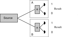
FIG. 1.: Schematic of a very generalized Bell experiment setup. After a source prepares two particles, these particles are directed out to the locations $A$ and $B$. At each location there is an analyzer with an adjustable parameters $\theta,\phi$. The particles are then detected resulting in a binary result “1” or “0” individually. These results can then be used to build up the statistics necessary to test the various Bell inequalities.

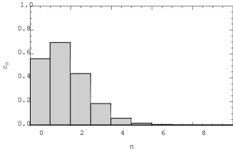
FIG. 2.: Plot of $c_{n}$ versus $n$

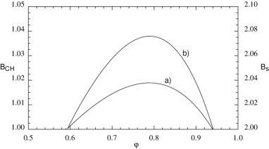
FIG. 3.: Plot of the Clauser Horne (a) and Spin (b) Bell inequality versus $\psi$. A violation occurs for the Clauser Horne Bell inequality if $B_{ch}>1$. A violation of the spin Bell inequality occurs for $B_{s}>2$.

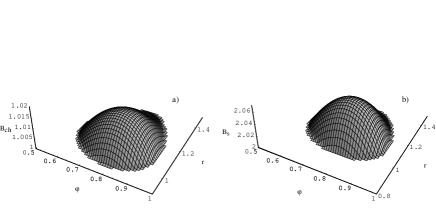
FIG. 4.: Plot of the Clauser Horne (a) and Spin (b) Bell inequality versus $r$ and $\psi$. A violation occurs for the CH Bell inequality if $B_{ch}>1$. A violation of the Spin Bell inequality occurs for $B_{s}>2$.

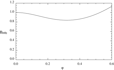
FIG. 5.: Plot of the information-theoretic Bell inequality versus $\psi$. A violation is possible for $B_{info}<0$.

TABLE I.: The optimal $c_{n}$ parameters to maximize the violation of the Clauser Horne and spin Bell inequalities. The $c_{n}$ values for the Gilchrist circle state are also given

n	$c_{n}$	Eqn (5) with $r\sim 1.12$
0	0.4990	0.5495
1	0.6355	0.6893
2	0.4760	0.4323
3	0.3135	0.1808
4	0.1465	0.0567
5	0.0235	0.0142
6	0.0075	0.0029
7	0.0024	0.0005
$B_{ch}$	1.019	1.016
$B_{s}$	2.076	2.064

REFERENCES

- [1] A. Einstein, B. Podolsky, and N. Rosen, Phys. Rev. 47, 777 (1935).
- [2] A. Gilchrist, P. Deuar and M. D. Reid , Phys. Rev. Lett. 80, 3169 (1998).
- [3] W. J. Munro and G. J. Milburn, Phys. Rev. Lett. 81, 4285 (1998)
- [4] B. Yurke and D. Stoler, Phys. Rev. Lett. 79, 4941 (1997).
- [5] E. S. Polzik, J. Carry, and H. J. Kimble, Phys. Rev. Lett 68, 3020 (1992)
- [6] J. F. Clauser, M. A. Horne, A. Shimony and R. A. Holt, Phys. Rev. Lett. 23, 880 (1969).
- [7] P. G. Kwiat, P. H. Eberhard, A. M. Steinberg and R. Y. Chiao, Phys. Rev. A 49, 3209 (1994).
- [8] M. Freyberger, P. K. Aravind, M. A. Horne and A. Shimony, Phys. Rev. A 53, 1232 (1995).
- [9] E. S. Fry, T. Walther, and S. Li, Phys. Rev. A 52, 4381 (1996).
- [10] By a strong test of quantum mechanics versus local realism, we mean a test in which no auxiliary assumptions are necessary.
- [11] G. S. Agarwal, Phys. Rev. Lett. 57, 827 (1986).
- [12] K. Tara and G. S. Agarwal, Phys. Rev. A 50, 2870 (1994).
- [13] M. D. Reid and L. Krippner 93, Phys. Rev. A 47, 552 (1993).
- [14] J. S. Bell, Physics (N.Y.) 1, 195 (1965).
- [15] J. F. Clauser and M. A. Horne, Phys. Rev. D 10 , 526 (1974).
- [16] J. F. Clauser and A. Shimony, Rep. Prog. Phys. 41, 1881 (1978).
- [17] M. D. Reid, Phys. Rev. A 40, 913 (1989)
- [18] S. L. Braunstein and C. M. Caves, Phys. Rev. Lett 61, 622 (1988).
- [19] M. Abramowitz and I. A. Stegun, Handbook of Mathematical Functions, Dover Publications Inc, Eighth Dover, New York, 1965
- [20] Checks were performed to ensure that truncation errors were minimal (less than ).