Abstract

A polynomial depth quantum circuit effects, by definition a poly-local unitary transformation of tensor product state space. It is a reasonable belief [Fy][L][FKW] that, at a fine scale, these are precisely the transformations which will be available from physics to solve computational problems. The poly-locality of discrete Fourier transform on cyclic groups is at the heart of Shor’s factoring algorithm. We describe a class of poly-local transformations, which include the discrete orthogonal wavelet transforms, in the hope that these may be helpful in constructing new quantum algorithms. We also observe that even a rather mild violation of poly-locality leads to a model without one-way functions, giving further evidence that poly-locality is an essential concept.

1 Introduction

Feynman [Fy] described how, in principle, a finite dimensional quantum mechanical system could be made to evolve so as to execute a sequence of $``$quantum gates.” By a quantum gate, we mean one of the several rather standard unitary operators applied to a small (usually 1, 2, or 3) number of tensor factors (and the identity on the remaining factors) within a larger tensor product of factors of bounded dimension, often taken to be $({\mathbb{C}}^{2})^{\otimes n}$. For example: NOT, Controlled NOT, and Controlled $i-$phase is known to be a complete basis [Ki].

Lloyd [L] made the converse explicit. Let $H$ be a poly-local Hamiltonian, $H=\overset{L}{\underset{\ell=1}{\sum}}H_{\ell}$ is a sum of $L\leq$ polynomial(problem size) terms $H_{\ell}$, each the identity except for a constant number of tensor factors. The Hamiltonian $H$ exponentiates to ${\bf U}=e^{2\pi itH}$ which is well approximated by ${\bf U}^{\prime}=\overset{M}{\underset{i=1}{\prod}}(\text{gate})_{i}$, where $M\leq\text{constant}\,\,t\cdot\frac{1}{\epsilon}\cdot L^{2}$ and $\epsilon>0$ is the allowed (operator norm) discrepancy between ${\bf U}$ and ${\bf U}^{\prime}$. The poly-local assumption on $H$ is very natural for most real world quantum mechanical systems and is often summarized by the axiom: $``$physics is local.” For example, in quantum field theory interactions tensors with more than four indices are generally not renormalizable. In more exotic contexts, such as, fractional quantum Hall systems [W] topological models have been proposed for which the Hamiltonian acting on internal degrees of freedom vanishes identically $H\equiv 0$, yet after a topological event, such as a braiding $b$ is completed, the internal state is transformed by ${\bf U}(b)$. For systems of this type (called: a unitary topological modular functor) a distinct argument was provided [FKW] that ${\bf U}(b)$ is poly-local. There seem to be few remaining candidates - perhaps quantum gravity - for a physical system having a finite dimensional state space whose evolution cannot be well approximated by a poly-local transformation ${\bf U}$. This reinforces confidence in the quantum circuit model QCM [Ki], and motivates the examination of (families of) transformations having a poly-local description. Any poly-local unitary transform is available as a $``$subroutine” on a quantum computer, but it will not generally be a simple matter to recognize a transformation as lying in (or efficiently approximated by) that class.

While a simple volume argument shows that only a tiny fraction of the unitary group ${\bf U}(2^{n})$ can be approximated (up to phase) by poly-local transformations, it is not known how to give concrete examples which cannot be thus approximated. The situation is reminiscent of the fact that transcendental numbers are easily seen to predominate, but less easy to identify. To add to the puzzle, in most contexts, we will be free to add ancilli to create an inclusion $v\mapsto v\,\otimes\mid 0\dots 0>$, $H\subset H^{+}$ of one Hilbert space into a larger one. It seems likely that there may be an operator $T:H\longrightarrow H$ which is not well approximated by poly-local operators but its extension $T\otimes\text{id}:H^{+}\longrightarrow H^{+}$ is. In this regard, Michael Nielsen has pointed out (private communication and Chpt. 6 [CN]) that the exponential of any Hamiltonian which is a sum of polynomially many product terms can, with the help of ancilli, be efficiently simulated on a quantum computer. There is no requirement on the individual product terms except that they be products, i.e. a tensors of operators each acting on one (or up to log many) qubit(s).

To appreciate the importance of a poly-local description consider the FFT. The reader familiar with the Fast Fourier Transform may be surprised that it has a virtue in the quantum context since it is already fast, $\mathcal{O}(N\log N)$, classically. But on this scale, we should think of the quantum version as poly$(\log N)$ in the sense that we may Fourier transform in poly$(\log N)$ time a data vector $\bigl{(}f(\mid 1>),\dots,f(\mid{N}>)\bigr{)}$ (held in superposition and previously computed in poly$(\log N)$ time) into its discrete Fourier transformation $\bigl{(}\widehat{f}(\mid\widehat{1}>),\dots,\widehat{f}(\mid\widehat{N}>)\bigr{)}$. The measurement phase of quantum computation samples the transform according to the density of its $L^{2}-$norm squared. In a sense, this is the best we could hope for in poly-log time. We could never output the entire transform in less than $\mathcal{O}(N)$ time, instead sampling shows us its sharpest spikes. Similarly with other transforms, a poly-local description allows us to sample, according to the $L^{2}-$ norm, that transform applied to any rapidly computable function.

A key step in the Shor factoring algorithm is his description of the discrete Fourier transform $F:C_{m}\longrightarrow\widehat{C}_{m}$ for the cyclic group of order $m$, where $m$ is a large smooth number, as a poly-local transform (The size parameter is $\log m$ so $F$ must be written as a composition of poly$(\log m)$ many gates).

We construct another class of examples by showing that cyclic periodic near diagonal matrices are poly-local (Thm 1). The construction is direct - no ancilla qubits are used. As an application, we prove (Corollary 1) that all the standard orthogonal discrete wavelet transforms, in particular the Daubechies transforms $D_{2n}$ [D], are poly-local. I thank C. Williams for pointing out that he and A. Fijany previously obtained an explicit factoring of $D_{2}$( = Haar) and $D_{4}$ into quantum circuits [AW]. Our alternative approach has the usual virtues and demerits of abstraction.

Some perspective into the limitations poly-locality imposes on the poly-time computational class of the QCM, BQP, can be achieved by adjoining oracles. Let $\mathcal{O}_{n}:({\mathbb{C}}^{2})^{\otimes n}\longrightarrow({\mathbb{C}}^{2})^{\otimes n}$ be a $``$super-gate” which can be called upon in addition to gates to transform the computational state $\Psi$. It is clear that if $\mathcal{O}_{n}$ encodes the answer to a difficult (or even undecidable) problem $P_{n}$, $\text{QCM}^{\mathcal{O}}$ will be improbable strong: If $f_{n}:\{0,1\}^{n-1}\longrightarrow\{0,1\}$ is a function and $\wedge(f_{n}):\{0,1\}^{n}\longrightarrow\{0,1\}^{n}$ is defined by $\wedge f_{n}(x_{1},\dots,x_{n-1},x_{n})=\{x_{1},\dots,x_{n-1},f_{n}(x_{1},\dots,x_{n-1})+x_{n}\}$ and $\mathcal{O}_{n}$ is the linear extension of $\wedge f_{n}$ operating on $({\mathbb{C}}^{2})^{\otimes n}$, then we can compute $f_{n}(x_{1},\dots,x_{n-1})$ by measuring the last qubit of $\mathcal{O}_{n}(x_{1},\dots,x_{n-1},0)$. However, if we stipulate that $\mathcal{O}_{n}$ is $``$locally-poly” meaning that the $(i,j)$ entry of $\mathcal{O}_{n}$ be computable in poly$(n)$ time, can the nonlocal structure of such $\mathcal{O}_{n}$ by virtue of their size alone, extend QCM? The following observation is evidence that the answer is $``$yes.”

Observation 1.

For each family of bijections $f_{n}:\{0,1\}^{n}\longrightarrow\{0,1\}^{n}$ which is computable in polynomial(n) time there is a family of oracles $\mathcal{O}_{n}$ with entries $(\mathcal{O}_{n})_{i,j}$ computable in poly$(n)-$time so that $f^{-1}$ can be computed by $\text{BQP}^{\mathcal{O}_{n}}$. Simply set $(\mathcal{O}_{n})_{i,j}=\delta_{f{(i),j}}$. Write the bit string $(y_{1}^{j},\dots,y_{n}^{j})=\overset{{\rightharpoonup}}{y}=y^{j},1\leq j\leq 2^{n}$. Then $\mathcal{O}_{n}\overset{{\rightharpoonup}}{y}=\overset{2^{n}}{\underset{j=1}{\Sigma}}\delta_{f(i),j}\,y^{i}=y^{f^{-1}(j)}=f^{-1}(\overset{{\rightharpoonup}}{y})$, so applying $\mathcal{O}_{n}$ to $(y_{1},\dots,y_{n})$ and then measuring each qubit separately solves the inversion problem $\mathcal{O}_{n}(y_{1}^{j},\dots,y_{n}^{j})=\big{(}y_{1}^{f^{-1}(j)},\dots,y_{n}^{f^{-1}(j)}\big{)}$. Thus, one-way functions disappear if we are permitted to adjoin locally-poly yet non-poly-local oracles. We have not succeeded in solving an $NP$ complete problem with such an oracle.

2 Periodic Band-Diagonal Transforms

It is common in signal processing to encounter smoothing operators which when written as matrices are band diagonal. Often mathematical reasons suggest wrapping the interval into a circle and considering cyclically banded matrices $M$, $M_{i,j}=0$ unless $\mid i-j\mid<b\mod N,1\leq i,j\leq N$. Two additional conditions natural in signal processing are unitary, $(M^{-1}=M^{\dagger})$ and cyclicity $\bigl{(}\exists k<<N\,\,\text{s.t.}\,\,M_{i,j}=M_{i+k,\,\,j+k}$, addition of indices taken $(\text{mod}N)\bigr{)}$. All these conditions occur in quadrature mirror filters [P]. We fix $b$ and $k$ and considering $N$ as parameter approaching infinity for studying the family of $N\times N$ matrices $M_{N}$. To summarize the $M_{N}$ are $N\times N$ unitary matrices, $b-$band diagonal in the cyclic sense, cyclic with period $k$, $k|N$, and $4b<N$. Furthermore even among different $M_{N}$, $M_{N^{\prime}}$, we assume $(M_{N})_{i,j}=(M_{N^{\prime}})_{i^{\prime},j^{\prime}}$. If $i\equiv i^{\prime}$ and $j\equiv j^{\prime}\mod k$, so the matrices look locally identical. Purely for convenience, we also assume all $N$ are powers of $2$, $N=2^{n}$, $n>n_{\circ}$ some fixed constant and $k=2^{\ell}$, this makes the fit with qubits effortless. A final technical assumption is necessary to efficiently approximate even a small $M_{N_{\circ}}$, $N_{\circ}=2^{n_{\circ}}$, from gates available in the QCM. It is sufficient here [Ki] to require the entries $M_{i,j}$ are algebraic numbers. This prevents some difficult to obtain information being encoded in the entries themselves. The theorem below asserts that the family $\{M_{N}\}$ is poly-local in the strictest sense: No ancilla are introduced to stabilize the problem.

Theorem 2.1.

Let $\{M_{N}\}$ be as above, there is a polynomial $p$ so that for any $\epsilon>0$ there is an $M^{\prime}_{N}$, $\epsilon$ close to $M_{N}$ in the operator norm, so that $M^{\prime}_{N}$ is a composition of $p\Bigl{(}n,\log\bigl{(}\frac{1}{\epsilon}\bigr{)}\Bigr{)}$ gates in the QCM.

Proof 2.2.

It is sufficient to consider $N=2^{n}$, for $n$ greater than any fixed number, so the reader may image $M_{N}$, $N$ comfortably large. For some $K=2^{j}k$, some $j>0$, we will modify $M_{N}$ to $\overline{M}_{N}$ to a unitary $K-$cyclic matrix which agrees with $M_{N}$ except $K-$periodically for a small (order $b$) slab of rows where $\overline{M}_{N}$ agrees with the identity matrix and a small (order $b$) transition region between the two types of rows.

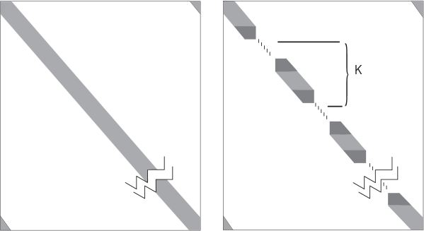
$M_{N}$           $\overline{M}_{N}$

Figure 1: White = zero, light shading = original K-periodic entries, dark shading = transition rows, and 1 = one.

The construction of $\overline{M}_{N}$ is very similar to the truncation process given in [F,P] so we will not give formulas here, but simple principles from which $\overline{M}_{N}$ may be constructed. Let $V_{I}$ be the vector subspace spaned by the rows of $M_{N}$ whose row index lies in $I$ (We think of $I$ as an interval with integer end points on the circle consisting of $R/NZ$). Let $W_{I}$ be the subspace spanned by the basis vectors with indexes in $I-$equivalently those rows of the identity $N\times N-$matrix. From the nonsingularity of unitary matrices we obtain:

Lemma 2.3.

Whenever $J$ contains the $b-$neighborhood of $I$, $W_{I}\subset V_{J}$ and $V_{I}\subset W_{J}.\,\,\square$

We apply the lemma several times below: consider an interval $I$ of $\ell>2b$ rows and a larger interval $J$ of $\ell\,\,\text{rows}+2b$ rows containing $I$ symmetrically. Let $J^{+}$ and $J^{-}$ denote the intervals of length$=2b$ at containing the $+$ and $-$ end points of $J$ respectively. The rows $\{q\}$ of $M_{N}$ in the complement of $I$ together with the rows $\{s\}$ of the identity matrix in the interval $J$ span the entire space. Let $\{r\}$ denote the rows of $M_{N}$ with indices in $J^{+}$ and $J^{-}$. The Gram-Schmidt process applied to $\{r\}\cup\{s\}$ (The Gram-Schmidt process requires an ordering; work from the middle of the $J$ interval outward) produces a Hermitian- orthogonal frame $\{t\}$ for the space spanned by $\{r\}\cup\{s\}$ (Note: $\{q\}\cup\{r\}\cup\{s\}$ span the entire space). This process naturally leaves the central $\ell-2b$ rows of $\{s\}$ unchanged, i.e. they remain standard basis vectors. The geometry of this process is pictured below.

Figure 2

The frame $\{t\}$ consists of $\ell$ standard basis vectors together with $2b$ vectors of length $\leq 2b$. Think of these $2b-$vector as mediating a transition from rows $\{q\}$ of $M_{N}$ to rows $\{s\}$ of the identity matrix. The truncation process preserves unitarity and band diagonality and the band width.

$\overline{M}_{N}$ is block diagonal consisting of $2^{n-j-\ell}$ identical blocks $\overline{M}$ (independent of N) down the diagonal. Thus, $\overline{M}_{N}$ has a tensor decomposition $\overline{M}_{N}=\overline{M}\otimes\text{id}_{({\mathbb{C}}^{2})^{\otimes n-j-\ell}}$.

Define $\overline{\overline{M}}=(\overline{M}_{N})^{-1}M_{N}$. Clearly the rows of $\overline{\overline{M}}_{N}$ agree with the identity matrix outside the $J-$intervals and $\overline{\overline{M}}_{N}$ is $b-$band diagonal. Thus, $\overline{\overline{M}}_{N}$ can be written in a tensor product form as well: $\overline{\overline{M}}_{N}$ consists of identical blocks down the diagonal of size $K$ provided $K\geq 2b$. Thus, we may write $\overline{\overline{M}}_{N}=P\circ(\overline{\overline{M}}\otimes\text{id}_{({\mathbb{C}}^{2})^{\otimes n-j-\ell}})\circ P^{-1}$ where $P$ is a cyclic permutation matrix of $\{1,2,\dots,N\}$. The permutation must arise since the blocks of $\overline{\overline{M}}$ are off-set from the blocks $\overline{M}_{N}$ by a translation of $\frac{K}{2}$.

Because we assumed the entries of $M_{N}$ to be algebraic so are the entries of $\overline{M}$ and $\overline{\overline{M}}$. It is well-known that algebraic numbers can be efficiently computed using Newton’s method so that refining the numerical accuracy of an algebraic $\alpha$ to up to a factor of $(1+\epsilon)$ requires only constant$(\alpha)\cdot$ poly $\log\bigl{(}\frac{1}{\epsilon}\bigr{)}$ computational steps. Now by a theorem of [Ki] for approximating a unitary transformation in a fixed dimension as a product of gates, we find matrices $\overline{M}^{\prime}$ and $\overline{\overline{M}}^{\prime}$, $|\overline{M}-\overline{M}^{\prime}|<\frac{\epsilon}{2}$, and $|\overline{\overline{M}}-\overline{\overline{M}}^{\prime}|<\frac{\epsilon}{2}$ using the operator norms, with $\overline{M}^{\prime}$ and $\overline{\overline{M}}^{\prime}$ a product of poly $\log\bigl{(}\frac{1}{\epsilon}\bigr{)}$ elementary gates.

The cyclic permutation $P$ and its inverse $P^{-1}$ are, of course, poly$(n)=\text{poly}(\log N)$ time computable classically. Writing $|x>\in\{1,2,\dots,N\}$ in an initial register and $|0>$ in an equal large (size $=n$, $N=2^{n}$) register of ancilli a well-known sequence of operations effects the transformation:

$$\begin{matrix}P_{i}(|x>\otimes|0>)\,\,\overrightarrow{\text{compute}P}\,\,\bigl{(}|x>\otimes|\,0+P(x)>\bigr{)}\,\,\overrightarrow{\text{flip}}\,\,\bigl{(}|P(x)>\otimes|x>\bigr{)}\\ \overrightarrow{\text{compute}P^{-1}}\,\,\bigl{(}|P(x)>\otimes|x+P^{-1}P(x)>\bigr{)}\\ =\big{(}|P(x)>\otimes|0>\big{)}\end{matrix}$$

(where $+$ denotes bit wise mod $2$ sum in the register). More directly, it is possible to build size $\mathcal{O}(n^{2})$ circuits from $``$NOT, $``$Controlled NOT,” and $``$swap” gates (See Section 2.4 [AW].), which use no ancilli and implement addition of $\frac{K}{2}$ modulo $N$. For example, a circuit implementing $+2\mod(8)$ is shown below.

Figure 3

Thus, all the 4 terms of an $\epsilon-$approximation $M^{\prime}_{N}$ may be written as a product of poly $(n,\log\frac{1}{\epsilon})$ many gates: $M_{N}\overset{\epsilon}{\approx}M^{\prime}_{N}=(\overline{M}^{\prime}\otimes\text{id})\circ P\circ(\overline{\overline{M}^{\prime}}\otimes\text{id})\circ P^{-1}$. $\square$

3 Wavelets

We define a discrete wavelet transform as the result of the pyramid algorithm [M] - applied to a band diagonal quadrature mirror filter. Daubachies’ [D] original basis is recovered by choosing a quadrature mirror filter whose
differencing rows have a maximal number of vanishing moments (consistent with orthogonality relations). For example, the simplest Daubachies wavelet Daub₄ is built from an orthogonal matrix(and mirror filter):

$$M_{N}=\overbrace{\begin{vmatrix}C_{1}&C_{2}&C_{3}&&&&&C_{0}\\ -C_{2}&C_{1}&-C_{0}&&&&&C_{3}\\ &C_{0}&C_{1}&C_{2}&C_{3}\\ &C_{3}&-C_{2}&C_{1}&-C_{0}\\ \vdots&&\vdots&&&&\vdots\\ &&&C_{0}&C_{1}&C_{2}&C_{3}\\ &&&-C_{3}&C_{2}&C_{1}&-C_{0}\\ C_{3}&&&&&C_{0}&C_{1}&C_{2}\\ -C_{0}&&&&&-C_{3}&C_{2}&C_{1}\\ \end{vmatrix}}^{2^{n}=N}\Biggr{\}}2^{n}=N$$

satisfying moment conditions:

$$C_{3}-C_{2}+C_{1}-C_{0}=0\;\;\text{and}\;\;0C_{3}-1C_{2}+2C_{1}-3C_{0}=0.$$

First let us explain in algorithmic terms how the wavelet coefficients of an data (column) vector $X=(x_{1},\dots,x_{N})$ are computed starting from a filter $M_{N}$ as above (compare [P]). The even components of $M_{N}X$ are regarded as $``$smoothed” and these are set aside for further processing. The odd components of $M_{N}X$ are the finest scale wavelet coefficients. To continue processing apply the matrix identical in description to $M_{N}$, but of half the size to the even output of $M_{N}X:M_{N/2}\bigl{(}\text{even}(M_{N}X)\bigr{)}$. Again set the even output aside: the odd output are the wavelet coefficients at the next-to-smallest scale. Now apply $M_{N/4}\Bigl{(}\text{even}\bigl{(}M_{N/2}(\text{even}M_{N}X)\bigr{)}\Bigr{)}$, etc… The process must terminate when $M$ becomes so small that wrapping around of rows threatens unitarity. For Daub<sub>4</sub> the last $M$ will be a $4\times 4$ matrix. The wavelet coefficients of $X$, usually written as $X$ integrated against a function $\psi$, are the output of the final differencing (proceeded, possible, by several smoothings). The $``$mother” or $``$scaling” coefficients will be the output of successive smoothings (i.e. even rows). These are traditionally written as $X$ integrated against a function $\phi$; there will be two of these for Daub₄.

The pyramid algorithm consist of only $\log(N)$ many applications of a filter matrix $M$, obeying the hypotheses of the theorem, and some easily computed permutations needed to sort out the even from odd rows between applications of $M$. Thus from the theorem, we have an evident corollary, which should be compared with the constructions of [AW] and [Kl].

Corollary 1.

Consider a poly-time computable function of $f$ from the integers $[1,\dots,N]$ into a fixed basis of a vector space $V$ of dimension $=d$. The function $f$ is recorded by a vector $v_{f}\epsilon V^{N}$. For any discrete (algebraic) wavelet transform $T$ applied to $f$, there is a quantum circuit, without ancilla, of length poly$\big{(}\log N,\,\log\frac{1}{\epsilon}\big{)}$ which yields a state space vector $T^{\prime}(v_{f})\epsilon V^{N}$ which is within $\epsilon>0$ of the exact transform $T(v_{f})$. The components of $T^{\prime}(V_{f})$ can be sampled by von Neumann measurement according to the density $|\text{component}_{i,j}|^{2}$, $1\leq i\leq N$, $1\leq j\leq d$.

The proceeding recipe, in so far as repeated smoothing is applied, sends a $``$Dirac function” $\delta$ toward a fixed point of the iteration $\phi(x)\longrightarrow\Sigma c_{n}\phi(2x-n)$. Such a fixed function $\phi$ is called the scaling function of the filter $M$. Wavelet coefficients (in the limit) correspond to integrations against $\psi(2^{k}x-n)$ where $\psi(x)=\Sigma(-1)^{k}c_{1-k}\phi(2x-k)$. Whereas, the Fourier transform efficiently extracts information about periodicity (hence its relevance to divisibility and factoring questions) the wavelet transforms (discrete or continuous) extract qualitatively different information. It is less easy to say precisely what combinatorial structures wavelets are best suited to detecting, but the answer must relate to phenomenon with a certain amount of both spacial and frequency localization. Some studies suggest fractal behaviors, Hausdorff dimension, and the like are readily observed in wavelet bases. Thinking democratically, one should not prefer either Fourier or wavelet bases, but seek different problems which can be solved by sampling the density of one transform or the other. So far on the Fourier side there is discrete log, factoring, and the abelian stabilizer problem [S][Ki] - essentially similar applications of that transform, and no interesting quantum applications, yet known, for the wavelet transforms.

4 Continuum Versus Vectorized Transforms

Both Shors’ [S] use of the Fourier transform and our treatment of wavelet transforms concerns the $``$vectorized” transform: The function values of $x^{a}\mod(n)$ in Shor’s work and the values of $f$ mod$(d)$ in our corollary 1 are treated as independent basis vectors in an abstract vector space. The transforms do not treat similar function values similarly, but rather place each possible outcome of $f(t)$ into a separate bin. Thus, there is no notion of the continuum limit of these transforms as presently constituted and they should not be confused with their continuous relatives in signal processing. The property of a function $f$ on the integers having period $=d$ is invariant under arbitrary permutation (or vectorization) of the target. This fact is crucial to the efficacy of the Fourier transform in Shor’s algorithm. It is more difficult to see what portion of the information captured by a wavelet transform is invariant under target permutation or vectorization.

Although it seems that a continuous - as opposed to vectorized - Fourier transform is not as useful for factoring, their may be other quantum applications for the continuous version. In the case of wavelets, it is more likely that continuous rather than vectorized transforms will be important. In the following paragraph, we explain how to use phase coding of states to build efficient continuous versions of any transform $T$ (such as Fourier or wavelet) for which there is an efficient quantum circuit implementation of the vectorized version.

Let $F:[1,\dots,N]\longrightarrow[1,\dots,d]$ be a funtion and denote $t\in[1,\dots,N]$ as the variable. For $1\leq x\leq d$, we may define $f_{x}(t)=0$ if $f(t)\neq x$, and $f_{x}(t)=1$ if $f(t)=x;\,\,f(t)=\overset{d}{\underset{x=1}{\Sigma}}f_{x}(t)$. A $``$vectorized” unitary transform obeys:

$$T\Bigl{(}\overset{N}{\underset{t=1}{\Sigma}}|t>\otimes|f(t){>}\Bigr{)}=\overset{d}{\underset{x=1}{\Sigma}}\,\,\overset{N}{\underset{\widehat{t}=1}{\Sigma}}\Bigl{(}T(f_{x})\widehat{t}\Bigr{)}|\widehat{t}{>}\otimes|x>$$

where $1\leq\widehat{t}\leq N$ is the transform variable, and states are written without numerical normalization factors. If we pick $D>>d$ and let $w=e^{2\pi\,i/D}$, the set of complex numbers $S=\{w^{i}|1\leq i\leq d\}$ is a short discretized arc of a circle and is a rather good affine model for $\triangle=[1,\dots,d]$ under the bijection $\delta\overset{b}{\rightarrowtail}e^{2\pi i\,\delta/D}$. After linear rescaling the quasi-isometric distortion of b is $\mathcal{O}\Bigl{(}\big{(}\frac{d}{D}\big{)}^{2}\Bigr{)}$ (A map $g:X\longrightarrow Y$ between metric spaces is said to have quasi-isometric distortion $\leq K$ for some $K\geq 0$ iff:

$$\frac{1}{1+K}\,\,d\big{(}g(x_{1}),g(x_{2})\big{)}\leq d(x_{1},x_{2})\leq(1+K)d\big{(}g(x_{1})g(x_{2})\big{)}.$$

We will neglect this distortion and code the values of a bounded real function $h:[1,\dots,N]\longrightarrow\big{[}0,\frac{2\pi d}{D}\big{]}$ into $\widetilde{h}:[1,\dots,N]\longrightarrow\bigtriangleup$, $\widetilde{h}=b^{-1}\circ r\circ\text{exp}(ih)$ where $r$ rounds to the nearest element of the form $e^{2\pi i\,\delta/D}$. Now a continuous version $\widetilde{T}$ of $T$ applied to $\widetilde{h}$ is given by the formula:

$$\widetilde{T}\Bigl{(}\overset{N}{\underset{t=1}{\Sigma}}|t{>}\otimes|\widetilde{h}(t)>\Bigr{)}=\overset{d}{\underset{x=1}{\Sigma}}\,\,\overset{N}{\underset{t=1}{\Sigma}}w^{x}\Bigl{(}\widetilde{T}(f_{x})\widehat{t}\Bigr{)}|\widehat{t}>.$$

Note that there is a simple modification of a quantum circuit computing $T$ to one computing $\widetilde{T}$. Instead of simply recording the qubit $|x>$ by adding $x$ to a $D-$state register $R$ holding zero, the trick is to initialize $R$ to the superposition:

$$w^{0}|1>+w^{1}|2>+\dots w^{D-1}|D>.$$

Now adding $x$ to the above state simply changes its phase by a factor of $w^{x}$. Thus, the transform $\widetilde{T}$, possessing a natural continuum limit, can be sampled in the QCM with no more difficulty than the discrete version $T$. If quantum computers are built, such continuous transforms would find application in signal processing. Beyond these obvious applications, it is interesting to wonder what algorithmic potential lies in these continuum transformations.

References

- [AW] I. Fijany and C. WilliamsQuantum Wavelet Transforms: Fast Algorithms and Complete Circuits. quant-ph/9809004 (Presented: First NASA Int. Conf. on Quantum Computing and Communication, Palm Springs, CA, Feb. 17-21, 1998)
- [CN] I. Chuang and M. Nielsen, Quantum computation and Quantum information, Cambridge Univ. Press (a book to appear).
- [D] I. Daubachies Orthonormal bases of compactly supported wavelets. Comm. Pure Appl. Math. 41 (1988), no. 7, 909–996.
- [Fy] R. Feynman, Simulating physics with computers, Int. J. Theor. Phys. 21(1982), 467-488.
- [FKW] M. Freedman, A. Kitaev, and Z. Wang, Simulation of topological field theories by quantum computers, To appear quan-ph/—-.
- [FP] M. Freedman and W. Press, Truncation of wavelet matrices: edge effects and the reduction of topological control. (English. English summary) Linear Algebra Appl. 234 (1996), 1–19.
- [Ki] A. Kitaev, Quantum computations: algorithms and error correction, Russian Math. Survey, 52:61(1997), 1191-1249.
- [Kl] A.Klappenecker Wavelets and Wavelet Packets on Quantum Computers quant-ph/9909014.
- [L] S. Lloyd, Universal quantum simulators, Science, 273(1996), 1073-1078.
- [M] S.G. Mallat, A Theory for Multiresolution Signal Decomposition: The Wavelet Representation IEEE Trans. Pattern adn Analysis and Machine Intelligence, 37, 12, Dec. 1989, 674-693.
- [P] W. Press, Numerical Recopies in Cambridge University Press, Cambridge, 1999. pg. 544)
- [S] P. W. Shor, Algorithms for quantum computers: Discrete logarithms and factoring, Proc. 35th Annual Symposium on Foundations of Computer Science, IEEE Computer Society Press, Los Alamitos, CA, 124-134.
- [W] F. Wilczek, Fractional statistics and anyon superconductivity, World Scientific Publishing Co., Inc., (Teaneack, NJ) 1990.