COVARIANCE, CORRELATION AND ENTANGLEMENT

Abstract

Some new identities for quantum variance and covariance involving commutators are presented, in which the density matrix and the operators are treated symmetrically. A measure of entanglement is proposed for bipartite systems, based upon covariance. This works for two- and three- component systems but produces ambiguities for multicomponent systems of composite diemnsion. Its relationship to angular momentum dispersion for symmetric spin states is described.

1 Introduction

Several measures of entanglement [1] or quantum correlations have been proposed: some are associated with the preparation of the state, others with the process of purification or distillation [2] and yet others with the notion of mutual information or relative entropy [3]. In this paper we wish to suggest another measure, based on covariance, in which the acts of state creation and observation are considered in a dual manner.

In practice it is very natural to describe the condition of the system (its method of preparation or lack of it) in terms of a density matrix which is tied to the subsequent observations on it. This is how the linkage between observer and observed occurs quantum mechanically, and of course the results are expressed in terms of traces over appropriate functions of the density matrix and of the operators being measured [4]. Indeed Mermin [5] has taken that view that the density matrix, and the correlations between observables which thereby ensue, constitute all of physical reality.

In this paper we will also focus on the density matrix. Because binning of observations is a necessity in practice, the dimension of the density matrix is thereby determined: $N$ separate bins produce a density matrix $\rho$ that is an $N\times N$ hermitian matrix, satisfying the usual hermiticity and trace conditions. In this way, we can regard the basis as an $N$-level system, rather like a particle of angular momentum $J=(N-1)/2$. Hence, although we might be studying the probability distribution of an observable which actually possesses a continuous spectrum, we can still regard it as a spin-like system; in practical terms, the bigger the binning number $N$, the greater the precision of the information about the continuous variable, but obviously $N$ is never infinite. For spin measurements, we need not go to such pains because $N$ is fixed for us at the start.

With the focus on density matrices, we will carry out measurements (without mutual interference) on two subsystems, 1 and 2 say, so their corresponding observables, superscripted by (1) and (2), are commuting operators. The system will be separable [6] or “disentangled” if the larger density matrix $\rho$ is merely a direct product of density matrices associated with the two subsystems, or $\rho=\rho^{(1)}\otimes\rho^{(2)}$; a particular case arises when the initial or prepared state is the direct product of two subsystem states, $|\psi\rangle=|\phi^{(1)}\rangle|\chi^{(2)}\rangle$. When two subsystems are disentangled, the results of measuring any quantity $A^{(1)}$ in the first subsystem are not tied to the results of measuring any quantity $B^{(2)}$ in the second subsystem; necessarily

$$\langle A^{(1)}B^{(2)}\rangle=\langle A^{(1)}\rangle\langle B^{(2)}\rangle,$$

for all choices of $A$ and $B$. However, if $\rho\neq\rho^{(1)}\otimes\rho^{(2)}$, the configuration is non-factorizable and the covariance,

$${\rm cov}(A^{(1)}B^{(2)})\equiv\langle A^{(1)}B^{2)}\rangle-\langle A^{(1)}\rangle\langle B^{(2)}\rangle,$$ (1)

no longer disappears.

The real issue is how to quantify the entanglement or lack of factorizability [6] of the larger density matrix. Several proposals have been advanced in the literature, but none of them is entirely simple or definitive [1]. However all researchers in this field seem to agree on the following three conditions for an entanglement measure $E(\rho)$:

1. $E(\rho)=0$ iff $\rho$ is separable, ie if the density matrix can be written as $\rho=\sum_{i}p_{i}\rho^{(1)}_{i}\otimes\rho^{(2)}_{i}$.

2. Local unitary transformations should leave $E(\rho)$ invariant.

3. $E(\rho)$ should not increase under local measurement and classical communication procedures, we intuitively know that such procedures cannot add non-locality characteristics to the system being measured.

As an extra requirement, it would be nice if $E(\rho)$ gave some indication of the extent of violation of Bell-type inequalities [4].

In this paper we want to put forward a concrete scheme for quantifying correlations between two subsystems and their possible entanglement. The scheme is based on a generalization of eq. (1) and particular choices of operators $A^{(1)}$ and $B^{(2)}$, which are readily applicable and rooted in the density matrix notion. In the next section we discuss several matters connected with non-separability of states and their influence on subsequent subsystem measurements. Because we deal with practical observations, the density matrix is truly discrete and we can assume that the elements of the vector space on which it lives have equal weight. As already mentioned, one may regard the dimension $N=N^{(1)}+N^{(2)}$ as corresponding to a “spin system”, with each component carrying equal weight, and can adopt the same stance for the subsystem dimensions $N^{(1,2)}$. (This restriction can be relaxed if the components have unequal weights, such as atomic energy levels at a finite temperature.)

The next section deals with the generalities of simultaneous measurements and their covariance properties [10]. This is followed by our suggestion for quantifying entanglement of two subsystems within a larger entity, which is shown to be consistent with normal expectations for two spin 1/2 subsystems, when $N^{(1)}=N^{(2)}=2$. We also discuss the use of total spin dispersion [7] as another measure of entanglement, with an allied appendix concerning the Majorana-Penrose [8] representation of spin states on the Poincaré sphere. The subsequent sections deal with entanglement measures for larger value of $N^{(1)}$ and $N^{(2)}$. Finally we discuss general questions pertaining to our suggested measure; these include Rovelli’s notion that information in quantum mechanics is relational [3], Mermin’s notions of correlations between local observables [5], and the difference between our modified correlation measure with classical correlations for impure states.

2 Correlations and density matrices

Elementary texts on quantum mechanics teach us that the results of all physical measurements and processes can be tied to the evaluation of traces of products of observables with the hermitian density matrix $\rho$. Thus statistical formulae like

$$\langle F\rangle={\rm Tr}(\rho F);\quad{\rm Tr}(\rho^{2})\leq 1,$$

etc.  are part of the standard repertoire. Of course, the $\rho$-eigenvalues lie between 0 and 1; in the latter case we are dealing with a pure state when the density matrix reduces to a projector $\rho\rightarrow P_{\psi}\equiv|\psi\rangle\langle\psi|$, while the most random situation $\rho=1/N$ corresponds to the case of maximum entropy.

The covariance for any two commuting observables $A,B$ in a mixed state $\rho$ is defined as

$${\rm cov}_{\rho}(A,B)\equiv\langle AB\rangle-\langle A\rangle\langle B\rangle={\rm tr}(\rho AB)-{\rm tr}(\rho A){\rm tr}(\rho B).$$ (2)

Clearly, ${\rm var}_{\rho}(A)={\rm cov}_{\rho}(A,A)$. Less well-known is the fact that pure state dispersions and correlations can be neatly expressed in terms of a single trace. Consider the quantity

$$C_{\rho}(A,B)\equiv{\rm tr}([\rho,A][B,\rho])/2={\rm tr}(\rho^{2}\{A,B\}/2-\rho A\rho B),$$ (3)

where $A$ and $B$ are any two operators. This quantity will be referred to as the alternative covariance .

We now present some elementary results about $C_{\rho}$ which follow simply from this definition:

1. $C_{\rho}(A,B)=C_{\rho}(A-a,B-b)$, where $a,b$ are any two constants.

2. $C_{\rho}(aA,bB)=abC_{\rho}(A,B)$.

3. $C_{\rho}(\sum_{i}A_{i},\sum_{j}B_{j})=\sum_{i,j}C_{\rho}(A_{i}.B_{j}).$

4. $C_{\rho}(A,A)={\rm tr}(\rho^{2}A^{2}-\rho A\rho A).$

5. $C_{U\rho U^{{\dagger}}}(A,B)=C_{\rho}(U^{{\dagger}}AU,U^{{\dagger}}BU)$, where $U$ is any unitary transformation. Thus a change of basis for the state is equivalent to an inverse change of basis for the operators.

6. $C_{\rho}(A,A^{{\dagger}})C_{\rho}(B,B^{{\dagger}})\geq|C_{\rho}(A,B^{{\dagger}})|^{2}$. This follows by considering the operator $T=[\rho,A-cB]$, with $c={\rm tr}([\rho,A][A^{{\dagger}},\rho])/{\rm tr}([\rho,A][B^{{\dagger}},\rho],$ and noting that ${\rm tr}(TT^{{\dagger}})\geq 0.$

7. $C_{\rho}(A,A^{{\dagger}})$ is real.

8. $|C_{\rho}(A,B)|^{2}$ is symmetrical under interchange, conjugation and change of phase of the two operators.

All of these properties are shared by the usual covariance cov${}_{\rho}(A,B)$. Nevertheless, alternative covariance $C_{\rho}$ does not provide an indication of variance and covariance in the usual sense. For instance, if the state is one of maximum entropy, on the one hand we have $C_{\rho}(A,B)=0$ for all $A,B$ because $\rho$ is proportional to unity; on the other hand, the ${\rm cov}_{\rho}(A,B)$ need not vanish.

Some special cases for the operators $A,B$ can now be studied.

1. If $A$ and $B$ commute, $C_{\rho}(A,B)={\rm tr}(\rho^{2}AB-\rho A\rho B).$

2. If $A$ and $B$ are both hermitian, $C_{\rho}(A,B)$ becomes real.

3. If $A$ and $B$ are both unitary, $C_{\rho}(A,A^{{\dagger}})={\rm tr}(\rho^{2}-\rho A\rho A^{{\dagger}})\leq{\rm tr}(\rho^{2})\leq 1.$ Likewise for $B$. Since $C_{\rho}(A,A^{{\dagger}})C_{\rho}(B,B^{{\dagger}})\geq|C_{\rho}(A,B^{{\dagger}})|^{2}$, it follows that $|C_{\rho}(A,B)|^{2}\leq 1.$

More particular cases arise when the system is prepared in a pure state $|\psi\rangle$, so that $\rho$ becomes a projection operator and $C_{\rho}(A,B)$ reduces to

$$C_{\rho}(A,B) \rightarrow \frac{1}{2}\langle\psi|\{A,B\}|\psi\rangle-\langle\psi|A|\psi\rangle\langle\psi|B|\psi\rangle=\frac{1}{2}\langle\{A-\langle A\rangle,B-\langle B\rangle\}\rangle$$ (4)

$$= {\rm cov}_{\rho}(A,B),\quad{\rm when~{}~{}}[A,B]=0.$$

Thus

$$C_{\rho}(A,A)\rightarrow\langle A^{2}\rangle-\langle A\rangle^{2}={\rm var}_{\rho}(A).$$ (5)

This is in keeping with the familiar variance-covariance inequality:

$${\rm var_{\rho}}(A){\rm var_{\rho}}(B)\geq|{\rm cov}_{\rho}(A,B)|^{2}.$$ (6)

If $A$ and $B$ are commuting unitary operators and because $|C_{\rho}(A,B)|^{2}\leq C_{\rho}(A,A)C_{\rho}(B,B)\leq({\rm tr}(\rho^{2}))^{2}\leq 1,$ we see that alternative covariance only attains a value of 1 for pure states.

It is worthwhile comparing the two covariance functions, in relation to two commuting observables, $A,B$. Since $[A,B]=0$, select an orthonormal basis $|i\rangle$ wherein the operators are simultaneously diagonalised, so

$$A=\sum_{i}|i\rangle a_{i}\langle i|,\quad B=\sum_{i}|i\rangle b_{i}\langle i|.$$

Then

$${\rm cov}_{\rho}(A,B) = {\rm tr}(\rho AB)-{\rm tr}(\rho A){\rm tr}(\rho B)$$

$$= \sum_{i}a_{i}b_{i}\langle i|\rho|i\rangle-\sum_{i,j}a_{i}b_{j}\langle i|\rho|i\rangle\langle j|\rho|j\rangle$$

$$= \sum_{i,j}a_{i}(b_{i}-b_{j})\langle i|\rho|i\rangle\langle j|\rho|j\rangle,$$

and similarly

$$C_{\rho}(A,B) = {\rm tr}(\rho^{2}AB)-{\rm tr}(\rho A\rho B)$$

$$= \sum_{i,j}a_{i}(b_{i}-b_{j})\langle i|\rho|j\rangle\langle j|\rho|i\rangle,$$

since $\sum_{j}\langle j|\rho|j\rangle={\rm tr}(\rho)=1$. Furthermore note that $\sum_{i,j}\langle i|\rho|j\rangle\langle j|\rho|i\rangle={\rm tr}(\rho^{2})\leq 1.$ Upon symmetrising the sums, we obtain the neater expressions,

$${\rm cov}_{\rho}(A,B)=\sum_{i,j}(a_{i}-a_{j})(b_{i}-b_{j})\langle i|\rho|i\rangle\langle j|\rho|j\rangle/2$$ (7)

$$C_{\rho}(A,B)=\sum_{i,j}(a_{i}-b_{j})(b_{i}-b_{j})\langle i|\rho|j\rangle\langle j|\rho|i\rangle/2$$ (8)

Whilst the ordinary covariance has a clear meaning—namely, a measure of the correlations between the results of local measurements $A$ and $B$ that commute—the interpretation of the alternative covariance is less obvious.

We can obtain more insight by choosing $A=B$. Since $\rho$ is a positive definite hermitian operator, $\langle i|\rho|i\rangle\langle j|\rho|j\rangle\geq\langle i|\rho|j\rangle\langle j|\rho|i\rangle$, for any two states $|i\rangle,|j\rangle$. Therefore for a general (mixed state) density matrix,

$$\sum_{i,j}(a_{i}-a_{j})^{2}\langle i|\rho|i\rangle\langle j|\rho|j\rangle\geq\sum_{i,j}(a_{i}-a_{j})^{2}\langle i|\rho|j\rangle\langle j|\rho|i\rangle,$$

or

$${\rm var}_{\rho}(A)\geq C_{\rho}(A,A).$$ (9)

In the light of the variance inequality above it is natural to ask whether

$$|{\rm cov}_{\rho}(A,B)|\geq|C_{\rho}(A,B)|$$

is true. In fact a single (but carefully chosen) counterexample suffices to show that it is false: in local bases $u,d$ for two local operators $A\otimes 1$ and $1\otimes B$, take

$$\rho=|(uu+dd)\rangle\langle(uu+dd)|/4+|ud\rangle\langle ud|/4+|du\rangle\langle du|/4$$

and select the local operators to be diagonal,

$$A\otimes 1 = (|uu\rangle\langle uu|+|ud\rangle\langle ud|)-(|du\rangle\langle du|+|dd\rangle\langle dd|)$$

$$1\otimes B = (|uu\rangle\langle uu|-|ud\rangle\langle ud|)-(|du\rangle\langle du|-|dd\rangle\langle dd|).$$

Evaluation of the two types of covariance leads to

$${\rm cov}_{\rho}(A,B)=0,\quad{\rm but}\quad C_{\rho}(A,B)=1/4.$$

Thus the variance inequality cannot be extended to covariance.

However, an immediate consequence of the inequality, var${}_{\rho}(A)\!\geq\!C_{\rho}(A,A)$, is that when var${}_{\rho}(A)=0$, $C_{\rho}(A,A)=0$ too for any observable $A$. But $2C_{\rho}(A,A)={\rm tr}([A,\rho][A,\rho]^{{\dagger}})$; so $[A,\rho]=0$, which means that $\rho$ is purely in an eigenstate of $A$. This accords with the basic tenets of quantum mechanics of course. The contrapositive of this result is that if $[A,\rho]\neq 0$, then ${\rm var}_{\rho}(A)>0$.

Another worthwhile comment stems from the observation that if $X$ is conjugate to $A$ in the sense $[A,X]=i\hbar$, then

$$2C_{\rho}(A,A)={\rm tr}\left([\rho,A][\rho,A]^{{\dagger}}\right)=\hbar^{2}{\rm tr}\left(\frac{\partial\rho}{\partial X}\frac{\partial\rho}{\partial X}^{{\dagger}}\right).$$

Thus,

$${\rm var}_{\rho}(A)=(\Delta A)^{2}\geq\hbar^{2}{\rm tr}\left(\left|\frac{\partial\rho}{\partial X}\right|^{2}\right)/2,$$

with equality only applying to pure states. For example, the energy uncertainty is given by $(\Delta H)^{2}\geq\hbar^{2}{\rm tr}\left(\left|\frac{d\rho}{dt}\right|^{2}\right)/2$, while the momentum uncertainty is given by the derivative of the density matrix with respect to position: $(\Delta P)^{2}\geq\hbar^{2}\;{\rm tr}\left(\left|\frac{\partial\rho}{\partial X}\right|^{2}\right)/2$, and so on.

For a general mixed configuration, the two inequalities,

$${\rm var}_{\rho}(A){\rm var}_{\rho}(B)\geq C_{\rho}(A,A)C_{\rho}(B,B)\geq\left|C_{\rho}(A,B)\right|^{2}$$

together with the well-known

$${\rm var}_{\rho}(A){\rm var}_{\rho}(B)\geq|{\rm cov}_{\rho}(A,B)|^{2},$$

provide a lower bound for the experimentally observed variance products of any two operators, whether or not they commute. For instance,

$${\rm var}_{\rho}(X).{\rm var}_{\rho}(P)\geq\left|\frac{1}{2}\hbar^{2}{\rm tr}\left(\frac{\partial\rho}{\partial X}\frac{\partial\rho}{\partial P}\right)\right|^{2}.$$

In the next section we present examples of operators $A,B$, for which there exist states such that $|{\rm cov}_{\rho}(A,B)|\geq|C_{\rho}(A,B)|$ and also other states for which $|C_{\rho}(A,B)|\geq|{\rm cov}_{\rho}(A,B)|$. Hence both inequalities must be considered jointly in an examination of the minimum of the variance product, together with Heisenberg’s well-known lower bound, $|{\rm tr}(\rho[A,B])|/2$.

3 Correlation measures for pure states of two subsystems

This section examines the correlation properties of the entanglement of two subsystems in a tensor product Hilbert space ${\mathbb{H}}^{(1)}\otimes{\mathbb{H}}^{(2)}$. By definition, measurements can be carried out without mutual interference on the two subsystems so their corresponding observables, superscripted by (1) and (2), are commuting operators. As mentioned in the introduction, a state of the system is factorisable or disentangled if the larger density matrix $\rho$ is merely a direct product of density matrices associated with the two subsystems, or $\rho=\rho^{(1)}\otimes\rho^{(2)}$. For any two local operators $A^{(1)}=A\otimes 1,B^{(2)}=1\otimes B$, it is easy to show that the covariance disappears:

$${\rm cov}_{\rho^{(1)}\otimes\rho^{(2)}}(A^{(1)},B^{(2)})=\langle(A-\langle A\rangle)\otimes\langle(B-\langle B\rangle)\rangle=0.$$ (10)

This includes the case of a pure disentangled state, $|\phi\rangle=|\phi^{(1)}\rangle|\phi^{(2)}\rangle$.

Having noted that the covariance is non-zero in disentangled states, we now refer to the conditions imposed upon any measure of entanglement. The second condition is that it be invariant under local unitary transformations. With this in mind, define the covariance entanglement for pure states as

$$E_{A^{(1)},B^{(2)}}(\rho)\equiv\max_{U=U^{(1)}\otimes U^{(2)}}|{\rm cov}_{U\rho U^{\dagger}}(A^{(1)},B^{(2)})|.$$

The maximum will clearly be invariant under additional local unitary transformations.

Since the operation of permuting the elements of a Hilbert space is unitary, all elements of the Hilbert spaces are equally important. For this reason, it is natural to select the operators $A^{(1)}$ and $B^{(2)}$ so as to equally weight the elements of the Hilbert space. The next section describes several ideas for achieving this, starting with the simplest case.

3.1 Pure state correlations for $N^{(1)}=N^{(2)}=2$

This section investigates a method for quantifying pure state entanglement in the simplest possible non-trivial case, corresponding to two spin 1/2 systems, with Hilbert space ${\mathbb{H}}\otimes{\mathbb{H}}$, where ${\mathbb{H}}={\mathbb{C}}^{2}$ is a local Hilbert space, with orthonormal basis $|u\rangle,|d\rangle$. Consider two local operators which distinguish between elements of the local Hilbert spaces. With the aim of weighting local basis elements equally, define operators in the product basis $|uu\rangle,|ud\rangle,|du\rangle,|dd\rangle$ by

$$A^{(1)}=\sigma_{3}^{(1)}=\!\left(\begin{array}[]{cccc}1&&&\\ &1&&\\ &&-1&\\ &&&-1\end{array}\right),B^{(2)}=\sigma_{3}^{(2)}=\!\left(\begin{array}[]{cccc}1&&&\\ &-1&&\\ &&1&\\ &&&-1\end{array}\right),$$

and so

$$A^{(1)}B^{(2)}=\sigma_{3}^{(1)}\sigma_{3}^{(2)}=\!\left(\begin{array}[]{cccc}1&&&\\ &-1&&\\ &&-1&\\ &&&1\end{array}\right).$$

Next consider the pure (normalized but arbitrary) state,

$$|\phi\rangle=\alpha|uu\rangle+\beta|ud\rangle+\gamma|du\rangle+\delta|dd\rangle.$$

Working out cov${}_{\rho}(A,B)$ in this state, it is straightforward to show that the covariance is maximised provided that $|\alpha|=|\delta|=1/\sqrt{2},\beta=\gamma=0$, or $|\beta|=|\gamma|=1/\sqrt{2},\alpha=\delta=0$. Thus one may take the four independent Bell states,

$$|10\rangle\equiv[|ud\rangle+|du\rangle]/\sqrt{2},\quad|00\rangle\equiv[|ud\rangle-|du\rangle]/\sqrt{2},$$

$$|1+\rangle\equiv[|uu\rangle+|dd\rangle]/\sqrt{2},\quad|1-\rangle\equiv[|uu\rangle-|dd\rangle]/\sqrt{2},$$

as the ones that have the largest covariance. (These pure states are also known to be the most entangled ones.) Of course they are all local unitary transforms of just one of them, say the Bell state, $|1+\rangle\equiv|(uu+dd)\rangle/\sqrt{2}$, with a corresponding $\rho=|uu+dd\rangle\langle uu+dd|/2$. If one rotates the operators $A,B$ together about the “$y$-axis” by the same amount, we can get a good idea of how the covariance varies with rotation angle; maximization is attained when the angle is $n\pi$. See Figure 1.

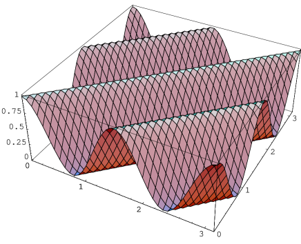
Figure 1: Equal-weight covariance of the Bell-state $|uu+dd\rangle/\sqrt{2}$ under equal local unitary transformations about two axes.

If a pure state is disentangled, then there is an orientation of the local $A^{(1)}$ which has zero variance. To see this, rotate the state by local unitary transformations until the reduced density matrix for the local operator in question is diagonalised. Since the initial state was pure and disentangled, then it may be represented by a separable projector $\rho=\rho^{(1)}\rho^{(2)}$, in which both reduced density matrices are projectors. Thus the main diagonals of $\rho^{(1)}$ and $\rho^{(2)}$ can be reduced to a single 1, with 0s elsewhere. Hence for diagonalised local operators $A$ and $B$ in this basis,

$$\langle A^{2}\rangle=\langle A\rangle^{2},\quad\langle B^{2}\rangle=\langle B\rangle^{2},$$

so the variances vanishes. Figure 2 illustrates the behaviour of the variance in a 2-variable parametrisation. The horizontal axis variable $x$ parametrises a set of pure states which range from disentangled to a maximally entangled Bell state, and back to disentangled again, i.e. $\rho=|\psi(x)\rangle\langle\psi(x)|$ where $|\psi(x)\rangle=\cos(x)|uu\rangle+\sin(x)|dd\rangle$. The second variable $y$ parametrises $y$-axis rotations of the local spin basis (1) associated with $A$ alone.

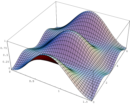
Figure 2: Equal-weight variance of a parametrised set of pure states, under different relative orientations of the state and the local operators. The maximally entangled states have $x=\pi/4$, and are the only states to attain a covariance of 1, whilst the disentangled states ($x=0,\pi/2$) are the only ones which attain a covariance of zero, for particular relative transformations of the local operator.

These results may be applied to actual spin measurements. If one knows that a state is pure, but is not certain of the degree of entanglement, local spin measurements can be made in a variety of directions. If the variance and covariance of these measurements vanishes in a pure state, then the state must be disentangled.

3.2 Pure state correlations for $N^{(1)}=N^{(2)}\equiv N>2$

Many different choices of local operators $A^{(1)},B^{(2)}$ are possible, and different choices will lead to different behaviour of the covariance. However before considering two sensible choices, let us note that for $N^{(1)}=N^{(2)}=2$, one of the maximally entangled states can be taken to be the state of total spin $|10\rangle$, while minimally entangled states are $|11\rangle,|1-1\rangle$. Now for these state combinations maximal entanglement happens to equate with maximal dispersion $(\Delta J)^{2}$ and zero entanglement equates with minimal dispersion $(\Delta J)^{2}$, where $J$ stands for total spin. This suggests that for higher spin, some maximally entangled states might be found by minimising the total angular momentum dispersion and vice versa. This approach towards quantifying entanglement is quite interesting in its own right and is pursued in Appendix A, where we also tie it to the Majorana-Penrose pictorial view of spin. In Appendix B, by contrast, we classify any measure of entanglement via an integrity basis for density matrix invariants.

3.2.1 Pair-discrimination

Consider two-system Hilbert spaces where the local spaces may each have dimension greater than 2. Select local operators $A^{(1)}=A\otimes 1,B^{(2)}=1\otimes B$, where $A,B$ may be expressed in their respective local bases as unitary transformations of the following diagonal matrix,

$$\left(\begin{array}[]{cccc}1&0&0&\cdots\\ 0&-1&0&\cdots\\ 0&0&0&\cdots\\ \cdots&\cdots&\cdots&\ddots\end{array}\right).$$ (11)

Next, maximise the covariance over all such unitarily-transformed matrices; the result is perforce invariant under local unitary transformations of the state. Labelling the local bases $|a_{i}\rangle$ and $|b_{i}\rangle$ respectively, where $i$ runs from 1 to $N$, operators like the above discriminate between pairs of elements in a local subspace of the full Hilbert space, and treat terms of the form $|a_{i}b_{k}+a_{j}b_{l}\rangle$ as the basic element of entanglement.

3.2.2 Equal weight unitary operators

Since we wish to handle all the subsystem states democratically, let us define an equal weight local unitary operator as consisting of some unitary transformation of a diagonal matrix comprising the $N$-th roots of unity. (Note that these matrices are not hermitian when $N\geq 3$ and cannot correspond to observables.) Here the local weight unitary matrices in their corresponding diagonalising basis, up to an overall phase, are given by

$$\left(\begin{array}[]{cccc}\exp(2i\pi/N)&&&\\ &\exp(4i\pi/N)&&\\ &&\ddots&\\ &&&1\end{array}\right).$$

Only for the spin $\frac{1}{2}$ $\times$ spin $\frac{1}{2}$ case, do these operators correspond exactly to the pairwise local unitary operators used previously. The next nontrivial case is $N=3$, or spin 1 $\times$ spin 1. In this case one can see that all states which are local unitary transformations of the pure state $|a_{1}b_{1}+a_{2}b_{2}+a_{3}b_{3}\rangle/\sqrt{3}$ have a maximal covariance of 1. To understand why, rotate the equal-weight unitary operators so that the local states $a_{1},a_{2},a_{3}$ and $b_{1},b_{2},b_{3}$ produce eigenvalues which are respectively conjugate pairs. This yields $\langle A^{(1)}B^{(2)}\rangle=1$. However, $\langle A^{(1)}\rangle=\langle B^{(2)}\rangle=0$, so the maximised covariance is 1.

What of other states, such as $|a_{1}b_{1}+a_{2}b_{2}\rangle$ when $N=3$? The following theorem gives a necessary and sufficient condition for a state to exhibit $C_{\rho}=1$, with respect to these equal weight operators and is in agreement with all other pure state entanglement measures.

Theorem: The only pure states which attain the maximised covariance of 1 under equal-weight local operators are states which are local unitary transformations of $|a_{1}b_{1}+a_{2}b_{2}+\ldots+a_{N}b_{N}\rangle/\sqrt{N}$. Any other states exhibit smaller correlations.

Proof: In a tensor product space ${\mathbb{H}}^{(1)}\otimes{\mathbb{H}}^{(2)}$, consider the state

$$|\psi\rangle=\sum_{i,j}c_{ij}|a_{i}b_{j}\rangle,$$

where $p_{ij}\equiv|c_{ij}|^{2}\geq 0$ and $\sum_{i,j}p_{ij}=1$, and the orthonormal bases $|a_{i}\rangle,|b_{j}\rangle$ are a complete set of eigenstates for the diagonalised equal-weight unitary operators $A^{(1)},B^{(2)}$, with eigenvalues $a_{k}=\exp(2i\pi k/N),b_{j}=\exp(2i\pi j/N)$ respectively. Recalling the result for such $A^{(1)},B^{(2)}$ that

$$(1-|\langle A^{(1)}\rangle|^{2})(1-|\langle B^{(2)}\rangle|^{2})\geq|\langle A^{(1)}B^{(2)}\rangle-\langle A^{(1)}\rangle\langle B^{(2)}\rangle|^{2},$$

we see that a maximised covariance of 1 is only attainable in a state where $\langle A\rangle=\langle B\rangle=0$, whereupon the covariance reduces to

$$C_{\psi}(A^{(1)},B^{(2)})=\left|\sum_{i,j}p_{ij}a_{i}b_{j}\right|.$$

In what cases is this expression maximised, subject to the condition that the mean values of the operators remain zero?

We are seeking to maximise $|\sum p_{ij}a_{i}b_{j}|$ subject to

$$\sum p_{ij}=1,\quad|\sum p_{ij}a_{i}|=0,\quad|\sum p_{ij}b_{j}|=0.$$

By the triangle inequality,

$$|\sum p_{ij}a_{i}b_{j}|\leq p_{11}|a_{1}b_{1}|+|\sum_{i,j>1}p_{ij}a_{i}b_{j}|\leq\ldots\leq\sum_{i,j}p_{ij}|a_{i}b_{j}|,$$

where equality holds at every stage only if all the complex numbers $a_{i},b_{i}$ have equal and opposite phase. This means that we are pairing $a_{i},b_{j}$ such that non-zero $p_{ij}$ (only for $i=j$) are associated in a one-to-one manner with $a_{i}b_{i}=1$ for all such pairs, otherwise the parallelism of the complex numbers will be lost. This will ensure that

$$\sum_{i}p_{ii}|a_{i}b_{i}|=\sum_{i}p_{ii}=1.$$

At the same time we have to guarantee that the average values of $A$ and $B$ vanish or $|\sum p_{ii}a_{i}|=0,|\sum p_{ii}b_{j}|=0$. Since $\sum_{i}a_{i}=\sum_{i}{b_{i}}=0$, a sufficient condition for this is that for all such pairs, the weightings are equal or $p_{ii}=1/\sqrt{N}$; in other words every $a_{i}$ and its corresponding $b_{i}=a_{i}^{*}$ only occurs at most once in the terms with equal non-zero weighting. (Actually one may introduce an arbitrary phase into $c_{ii}$ without affecting this conclusion, but we have chosen not to do so.)

Having established that the states which maximise the covariance can take the form $|a_{i}a_{1}^{*}+a_{2}a_{2}^{*}+\ldots\rangle$, we should point out that it is not necessary for all the terms to be paired up. Consider the case $N=4$, or spin $3/2\otimes$ spin $3/2$ systems, with bases $a_{1},\ldots,a_{4}$ and $b_{1},\ldots,b_{4}$ respectively. It is possible to attain maximised covariances of 1 under the equal-weight measures both for $|\psi\rangle=|a_{1}b_{1}+a_{2}b_{2}\rangle/\sqrt{2}$ and for $|\phi\rangle=|a_{1}b_{1}+a_{2}b_{2}+a_{3}b_{3}+a_{4}b_{4}\rangle/2$. This is achieved by choosing eigenvalues so that $\langle A^{(1)}\rangle=\langle B^{(2)}\rangle=0$ and yet pick eigenvalues such that the values of $A^{(1)}B^{(2)}$ in the states $|a_{1}b_{1}\rangle\ldots|a_{4}b_{4}\rangle$ are all 1. As we are in a 4-dimensional space, we can achieve this by taking the eigenvalue sets $\{1,-1\}$ and $\{1,i,-1,-i\}$ for both operators on both states $|\psi\rangle$ and $|\phi\rangle$ respectively.

This observation means that the ‘equal-weight’ $C$-based measures for $N>2$ are not measures of entanglement, under the standard criteria. Information-based entanglement measures, such as the relative entropy, specify that $|\psi\rangle$ is less entangled than $|\phi\rangle$. It appears that the covariance-based measures of entanglement are most useful when dealing with spin $\frac{1}{2}\otimes$ spin$\frac{1}{2}$ systems, since in this case there is no ambiguity as to the choice of eigenvalues. Similarly for operators of prime dimension, such ambiguities are absent, because there is only one way to arrive at a maximally correlated state: the non-uniqueness only pertains to composite-dimensional local spaces.

The above result demonstrates that for pure states, the reduced density matrices must be diagonalised in order to maximise the covariance of the diagonalised local unitary operators. However, for mixed states it is not at all obvious that the reduced density matrices must be diagonalised in order to maximise the unitary matrix covariance. This issue will will be examined in section 4.

3.3 Pure state correlations for $N^{(1)}\neq N^{(2)}$

For spaces of differing dimension, such as spin $1\times$ spin $1/2$, the covariance of the pairwise operators behave just as in the other cases. However, if the equal-weight local operators are used, covariances of 1 are not attainable. This reflects the fact that the bases have different sizes, and so there is no way to pair up elements between the bases in a one-to-one manner so as to produce a set of product eigenvalues with the same phase.

The simplest example which exhibits this effect is a spin $\frac{1}{2}\;\otimes$ spin $1$ space, with equal-weight operators

$$A^{(1)}={\rm diag}(1,-1)\otimes 1,\quad B^{(2)}=1\otimes{\rm diag}(1,\exp(2i\pi/3),\exp(4i\pi/3))$$ (12)

As with the proof that the states of maximum covariance are $|a_{1}b_{1}+\ldots+a_{n}b_{n}\rangle$, a covariance of 1 is only attainable if $\langle A^{(1)}B^{(2)}\rangle=1$; we also need the complex numbers $p_{ij}a_{i}b_{j}$ to have the same phase (where the state has Schmidt decomposition $|\phi\rangle=\sum_{ij}\sqrt{p_{ij}}|a_{i}b_{j}\rangle$ in the basis of eigenvalues of the operators $A^{(1)},B^{(2)}$). Following similar arguments to those used in the proof, it is not possible to choose $p_{ij}$ so that the direction condition is satisfied; this is because no repetitions of $a_{i}$ or $b_{j}$ values can occur in the set of non-zero $p_{ij}$, since the resulting $p_{ij}a_{i}b_{j}$ would not have the same phase. But it is not possible to partially pair up the given set of eigenvalues so that the directions of the products are the same, by straightforward enumeration of the cases. Thus states in this basis cannot attain covariances of $1$.

Clearly many other local operators can be defined which provide a variety of different correlation measures for two-system states but none stands out.

4 Correlation measures for mixed states

Making a distinction between quantum and classical correlations has proved a thorny problem in the study of quantum entanglement. The nature of the problem may be seen when comparing the two states, one pure and one mixed, which possess the same covariance for $A^{(1)}=B^{(2)}=\sigma_{3}$:

$$\frac{1}{2}|uu+dd\rangle\langle uu+dd|\quad{\rm and}\quad\frac{1}{2}|uu\rangle\langle uu|+\frac{1}{2}|dd\rangle\langle dd|.$$

The first state is a Bell state and is maximally entangled, whilst the second state is a mixture of disentangled projectors, and is normally regarded as being disentangled. As both states exhibit correlations, it is natural to ask whether the alternative covariance introduced in section 2 provides a way of distinguishing between classical and quantum correlations.

4.1 Distinction between $C_{\rho}$ and cov_ρ

Take any two commuting local measurements, $A^{(1)}=A\otimes 1,B^{(2)}=1\otimes B$, and define the function

$$E_{AB}(\rho)\equiv{\rm max}_{U}|C_{U\rho U^{\dagger}}(A^{(1)},B^{(2)})|^{2},$$ (13)

where the maximum is now taken over all local unitary transformations of the general mixed density matrix $\rho$. In previous sections we investigated the behaviour of this function for pure states (when $C_{\rho}$ reduces to the covariance), and found that it appeared to have many of the properties desirable in a pure state entanglement measure.

The situation where the density matrix corresponds to an impure configuration is more intriguing. Shown below is a comparison of the behaviour of the two maximised covariance entanglement measures, in several example configurations, which illustrate the distinction between $|{\rm cov}_{\rho}(A^{(1)},B^{(2)})|^{2}$ and $|C_{\rho}(A^{(1)},B^{(2)})|^{2}$.

Density matrix	$|{\rm cov}_{\rho}(A^{(1)}\!,\!B^{(2)})|^{2}$	$|C_{\rho}(A^{(1)}\!,\!B^{(2)})|^{2}$
$\rho_{1}=[|uu\rangle\langle uu|+|dd\rangle\langle dd|]/2$	1	0
$\rho_{2}=[\frac{1}{2}|uu\rangle\langle uu|\!+\!\frac{1}{4}|uu\!+\!dd\rangle\langle uu\!+\!dd|]$	3/4	1/4
$\rho_{3}=|uu\rangle\langle uu|$	0	0
$\rho_{4}=|uu\!+\!dd\rangle\langle uu\!+\!dd|/2$	1	1

The illustrative state $\rho_{4}$ is pure but entangled, $\rho_{3}$ is factorizable and therefore disentangled, while the matrix $\rho_{1}$ is not factorizable but can be expressed as a sum of separable projectors; therefore $\rho_{1}$ should represent a disentangled configuration, according to standard expectations. By inspecting the table we see that cov${}_{\rho}(A^{(1)},B^{(2)})$, being nonzero, is not a good entanglement measure $E(\rho)$, but the alternative $C_{\rho}(A^{(1)},B^{(2)})$ is better in that it does vanish.

The alternative covariance $C$ in mixed states is bounded above by ${\rm tr}(\rho^{2})$, so the state must be pure to obtain a covariance of 1 under local unitary transformations. Another point worth remembering is that for configurations of maximum entropy where $\rho\propto 1$ and commutes with all operators, $C$ is automatically zero.

Figures 3 and 4 depict the squares of the equal weight classical covariance and alternative covariance of a parametrised mixture of different Bell states. They show that both covariance measures attain a maximum of 1 only for the pure states, and that the behaviour of these functions depends upon the kind of Bell-states involved in the mixtures.

(i) $\left|{\rm cov}_{\rho}(A^{(1)},B^{(2)})\right|$

(ii) $\left|C_{\rho}(A^{(1)},B^{(2)})\right|$

Figure 3: (i) Equal-weight covariance magnitude of a parametrised mixture of different Bell-states. (ii) Equal weight alternative covariance magnitude for the Bell-state mixture. The parametrisation in both cases is any one of the following: $\rho=x|b_{1}\rangle\langle b_{1}|+(1-x)|b_{2}\rangle\langle b_{2}|,$ where either $|b_{1}\rangle=|ud\pm du\rangle/\sqrt{2}$, $|b_{2}\rangle=|ud\mp du\rangle/\sqrt{2}$, or else $|b_{1}\rangle=|uu\pm dd\rangle/\sqrt{2}$, $|b_{2}\rangle=|ud\mp du\rangle/\sqrt{2}$. The Bell-states must be different in these parametrisations, to obtain a non-trivial result. The result is not a maximisation over all local unitary transformations.

(i) $\left|{\rm cov}_{\rho}(A^{(1)},B^{(2)})\right|$

(ii) $\left|C_{\rho}(A^{(1)},B^{(2)})\right|$

Figure 4: (i) Equal-weight covariance magnitude of a parametrised mixture of different Bell-states. (ii) Equal weight alternative covariance magnitude for the Bell-state mixture. The parametrisation in both cases is $\rho=x|b_{1}\rangle\langle b_{1}|+(1-x)|b_{2}\rangle\langle b_{2}|,$ where $|b_{1}\rangle=|uu\pm dd\rangle/\sqrt{2},|b_{2}\rangle=|ud\pm du\rangle/\sqrt{2}$. The Bell states in these parametrisations may be used in any combination allowed by the above expression (i.e. all four sign combinations are permitted). The result is not a maximisation over all local unitary transformations.

For any choice of $A^{(1)},B^{(2)}$, a maximised $C_{\rho}(A^{(1)},B^{(2)})$ of zero occurs for many mixed configuration $\rho$ which are disentangled, according to the standard definition of a mixed state, such as the states of maximum entropy with $\rho\propto 1$. This behaviour of the alternative covariance for ‘partially entangled’ configurations is what one would naively expect for a mixed configuration entanglement measure $E(\rho)$. However, there is a particular class of mixed states which are disentangled according to the commonly accepted definition of a mixed state, whilst exhibiting non-zero alternative covariance properties.

4.2 Conditions on entanglement measures

This section assesses the alternative covariance as a measure of entanglement, according to the principles outlined by Vedral and Plenio[1].

Firstly, consider the cases where a state exhibits zero quantum correlation. A mixed configuration is usually defined to be separable if it can be written as a sum of separable projectors; thus

$$\rho=\sum_{j}p_{j}\rho^{(1)}_{j}\otimes\rho^{(2)}_{j};\qquad\rho_{i}^{(n)}\rho_{j}^{(n)}=\delta_{ij}\rho_{i}^{(n)}.$$

Then for any such $\rho$,

$$C_{\rho}(A^{(1)},B^{(2)}) = {\rm tr}(\rho^{2}A^{(1)}B^{(2)}-\rho A^{(1)}\rho B^{(2)})$$

$$= {\rm tr}\left(\left(\sum p_{i}\rho^{(1)}_{i}A\otimes\rho^{(2)}_{i}\right)\left(\sum p_{j}\rho^{(1)}_{j}\otimes B\rho^{(2)}_{j}\right)\right)$$

$$-{\rm tr}\left(\left(\sum p_{i}\rho^{(1)}_{i}A\otimes\rho^{(2)}_{i}\right)\left(\sum p_{j}\rho^{(1)}_{j}\otimes\rho^{(2)}_{j}B\right)\right)$$

$$= \sum\sum p_{i}p_{j}{\rm tr}(\rho^{(1)}_{i}A\rho^{(1)}_{j}\otimes\rho^{(2)}_{i}B\rho^{(2)}_{j}$$

$$\qquad\qquad\qquad-\rho^{(1)}_{i}A\rho^{(1)}_{j}\otimes\rho^{(2)}_{i}\rho^{(2)}_{j}B)$$

$$= \sum\sum p_{i}p_{j}{\rm tr}_{(1)}(\rho^{(1)}_{i}A\rho^{(1)}_{j}){\rm tr}_{(2)}(\rho^{(2)}_{i}B\rho^{(2)}_{j}-\rho^{(2)}_{i}\rho^{(2)}_{j}B)$$

$${\rm or} \sum\sum p_{i}p_{j}{\rm tr}_{(1)}(\rho^{(1)}_{i}A\rho^{(1)}_{j}-\rho^{(1)}_{i}\rho^{(1)}_{j}A){\rm tr}_{(2)}(\rho^{(2)}_{i}B\rho^{(2)}_{j}),$$

which is guaranteed to vanish if the $\rho_{i}^{(n)}$ are projectors.

Now consider cases where the density matrix is a mixture like

$$\frac{1}{2}|uu\rangle\langle uu|+\frac{1}{8}|(u+d)(u+d)\rangle\langle(u+d)(u+d)|.$$

Here, it can be shown that these mixtures produce non-zero $C_{\rho}(A,B)$, because their expansion into projector traces may be used to extract off-diagonal elements of observables $A,B$ in suitable local bases. Take for instance the two local operators on separate spin $\frac{1}{2}$ bases, $A\!=\!B\!=\sigma_{2}$, which is a unitary transformations of the equal-weight matrix, $\sigma_{3}$ used previously. The terms in the expansion of $C$ above are non-vanishing only if non-parallel, non-orthogonal projectors are used. Thus we evaluate the two non-vanishing terms, with local projectors $|u+d\rangle\langle u+d|/2,\;\;|u\rangle\langle u|$ giving

$$\langle u+d|u\rangle\langle u|A|u+d\rangle(\langle u|B|u+d\rangle\langle u+d|u\rangle-\langle u+d|B|u\rangle\langle u|u+d\rangle)$$

$$\qquad\qquad\qquad=(-i)(-i-i)=-2,$$

$$\langle u|u+d\rangle\langle u+d|A|u\rangle(\langle u+d|B|u\rangle\langle u|u+d\rangle-\langle u|B|u+d\rangle\langle u+d|u\rangle)$$

$$\qquad\qquad\qquad=(i)(i+i)=-2.$$

These terms do not cancel, and the other two terms in the expansion are zero, so the alternative covariance $C_{\rho}$ is non-zero even though we are dealing with a disentangled state, according to the usual terminology.

From this we deduce that the measure $E$ based on alternative covariance is not a measure of entanglement (according to the conditions provided by Vedral and Plenio), when mixed states are encountered, since it violates the first condition for such measures.

4.3 Local purification procedures

The third condition on entanglement measures proposed by Vedral and Plenio is that the entanglement of a state should not increase under the three types of purification processes (LGM, CC, and PS).

Let us consider all possible LGM, CC and PS measurement operations which act on a disentangled state

$$\rho_{0}=|uu\rangle\langle uu|$$

and yield states which exhibit non-zero quantum covariance $C_{\rho}(A^{(1)},B^{(2)})$, such as

$$\rho_{1}=\frac{1}{2}|uu\rangle\langle uu|+\frac{1}{8}|(u+d)(u+d)\rangle\langle(u+d)(u+d)|$$

The change from $\rho_{0}$ to $\rho_{1}$ may be performed by the classically correlated set of local measurements $V_{1}\ldots V_{8}$, where

$$V_{1} = \frac{1}{\sqrt{2}}|uu\rangle\langle uu|=\frac{1}{\sqrt{2}}|u\rangle\langle u|\otimes|u\rangle\langle u|$$

$$V_{2} = \frac{1}{2\sqrt{2}}|(u+d)(u+d)\rangle\langle uu|=\frac{1}{2\sqrt{2}}|(u+d)\rangle\langle u|\otimes|(u+d)\rangle\langle u|$$

together with $V_{3},\ldots,V_{8}$ which have $\langle ud|,\langle du|,\langle dd|$ in place of $\langle uu|$. Thus $\sum V_{i}\rho_{0}V_{i}^{\dagger}=\rho_{1}$, and $\sum V_{i}^{{\dagger}}V_{i}\propto 1$, so this represents a complete measurement.

Because this set of operations $V_{i}$ is local, we would expect any measure of entanglement to not increase under these operations. However, the state which results from this procedure does in fact exhibit non-zero $C_{\rho}$, as was demonstrated earlier. Therefore we have found a complete local general measurement for which the entanglement increases based upon alternative covariance. Thus the unitarily maximised $C_{\rho}$ does not satisfy the conditions for a measure of mixed state entanglement proposed by Vedral and Plenio.

5 Conclusion

We have shown that for pure two 2-state systems, the maximised covariance agrees with other measures of entanglement in specifying which states are disentangled and which are maximally entangled. For subspaces of larger dimension, the situation is less clear-cut since there are ambiguities in the process of selecting eigenvalues for the local operators, but it is possible to obtain information about the degree of higher-order correlations of two subsystems in this way.

The variance and covariance could be used to indicate the best measurements to make to detect entanglement of bipartite systems, by locating the unitary transformation which produces maximum covariance. However, the problem of mixed state separability measures is not resolved by the correlation functions $C$ and the covariance, as we have used them in this paper. Nevertheless the link between alternative variance and the conjugate variable derivatives for position, momentum, energy and time is intriguing, and might be extended to other quantised models involving conjugate variables. The inequality ${\rm var}(X)\geq C(X,X)$, with equality for pure states, should be applicable to situations where observations are made upon impure states.

It is interesting to observe that for pure density matrices $\rho$, both the average value and the variance of an operator $F$ are symmetrical under the interchange of $\rho$ and $F$, when expressed in the form

$$\langle F\rangle={\rm tr}(\rho F),\;{\rm var}(F)=C_{\rho}(F,F)={\rm tr}(\rho^{2}F^{2}-\rho F\rho F).$$

They motivate the suggestion that a quantum state $|\psi\rangle$ is best represented not as a ket, but as a projection operator $P_{\psi}=|\psi\rangle\langle\psi|$. Any measurement process on the state is relational in the sense of Rovelli [3]: the notion of state vector reduction is replaced by the notion that every new measurement process requires a new Hilbert space to be defined, with new operators corresponding to the new state and any successive measurement made upon the state. The basic idea is that a measurement treats the state information in a comparative sense, with meaning only in relation to the operator corresponding to the observable quantity being measured.

The process of state reduction to the eigenstate of some observable under a measurement is an apparent one resulting not from the action of the operator corresponding to the measurement, but from some other physical process which occurs in the measurement, such as a filtering process of some kind (like the case of a Stern-Gerlach experiment), causing later measurements on the physical system to be represented in a completely new basis by new state and measurement operators. The adoption of the projector as a unit of relational information does not change any predictions of quantum mechanics in terms of average values.

Appendix A The Majorana-Penrose Representation of Symmetrised States

It is well known that a spin state $|j,m\rangle$ can be obtained by forming a fully symmetric direct product of $n=2j$ spin 1/2 states. Denoting the spin 1/2 states by $|u\rangle=|1/2,1/2\rangle,\,\,|d\rangle=|1/2,-1/2\rangle$, the spin $j$ states are given by:

$$|j,j\rangle = |\overbrace{uu\ldots u}^{2j}\rangle$$

$$|j,j-1\rangle = [|du\ldots u+ud\ldots u+\cdots+uu\ldots d\rangle]/\sqrt{2j}$$

$$\cdots \cdots$$

$$|j,m\rangle = \sum_{\rm sym}|(u)^{j+m}(d)^{j-m}\rangle/\sqrt{{}^{2j}C_{j+m}}$$ (14)

$$\cdots \cdots$$

$$|j,-j\rangle = |dd\ldots d\rangle.$$

In the Majorana-Penrose representation [8] these states are mapped onto the unit sphere, with stereographic projection $z$ taken from the South Pole, onto the complex plane by making the association:

$$|j,m\rangle\leftrightarrow\sqrt{{}^{2j}C_{j+m}}z^{j+m}.$$ (15)

This association may be rewritten in terms of the spin-$\frac{1}{2}$ basis in an elegant way which emphasises that the $z^{i}$ powers are proportional to a symmetrised sum where $i$ spin-$\frac{1}{2}$ terms of spin $|u\rangle$, and $(n-i)$ spin $|d\rangle$ terms are selected, namely

$${}^{2j}C_{j+m}z^{j+m}\leftrightarrow|u\ldots ud\ldots d\rangle+\ldots+|d\ldots du\ldots u\rangle$$ (16)

where the sum is taken over all ways of selecting $i$ spin-$\frac{1}{2}$ elements from the $2j+1$ elements in the spin-$j$ space.

Thus from a general spin state $|\psi\rangle=\sum_{m}\psi_{jm}|jm\rangle$ we can define a polynomial

$$p(z)=a_{2j}z^{2j}+a_{2j-1}z^{2j-1}+\cdots+a_{0}1,$$

where $a_{j+m}\equiv\sqrt{{}^{2j}C_{j+m}}\psi_{jm}z^{j+m}$. The roots of this polynomial give $2j$ points on the stereographic plane and, correspondingly, a general spin $j$ state, being some superposition over $m$ values, will be described by $2j$ distinct points on the Poincaré sphere, obtained by stereographic projection of the roots placed on the horizontal $x$-$y$ plane. It is worth remarking that another spin state $|\psi^{\prime}\rangle$, represented by another polynomial,

$$p^{\prime}(z)=a^{\prime}_{2j}z^{2j}+a^{\prime}_{2j-1}z^{2j-1}+\cdots+a^{\prime}_{0}1,$$

yields a scalar product,

$$\langle\psi^{\prime}|\psi\rangle=\sum_{m}a_{j+m}a^{\prime*}_{j+m}/^{2j}C_{j+m}.$$

Figure 5: Majorana representation of the state with polynomial $(z-i)(z+i)$

In the case where the degree $m$ of the polynomial is less than $2j$, $2j-m$ additional points at the South pole (the projective point) are added to the projection, corresponding to ‘roots at infinity’. Figure 5 depicts an example of stereographic projection for the spin-$1$ state represented by the quadratic polynomial

$$p(z)=(z-i)(z+i)=z^{2}-1\leftrightarrow[|11\rangle+|1-1\rangle]/\sqrt{2}.$$ (17)

By contrast, for spin 1, the maximum and minimum spin states $|1,1\rangle$ and $|1,-1\rangle$ correpond to two repeated points at the North and South Pole, respectively; on the other hand the pure intermediate spin state $|1,0\rangle=|ud+du\rangle/\sqrt{2}$ corresponds to one point at the North pole and the other at the South pole. The Bell states, $|1,\pm\rangle\equiv|uu\pm dd\rangle/\sqrt{2}$ are also antipodal points, but are located around the equator, specifically at coordinates (1,0,0)& (-1,0,0) and (0,1,0) & (0,-1,0). Under all accepted measures of entanglement, the spin zero state $|0,0\rangle=|ud-du\rangle/\sqrt{2}$, the Bell states $|1,\pm\rangle$ and $|1,0\rangle$ (in fact, all local unitary transformations of these states) are maximally entangled. This suggests that taking the two points as “far apart as one another” on the Poincaré sphere is one possible way of producing maximal entanglement.

Another point of interest is that for these spin 1 states, the rotationally invariant dispersion measure,

$$(\Delta J)^{2}\equiv\langle\vec{J}.\vec{J}\rangle-\langle\vec{J}\rangle.\langle\vec{J}\rangle,$$

attains the maximum value of 2, because $\langle\vec{J}\rangle$ vanishes; so it also suggests that the quantity $(\Delta J)^{2}/\langle\vec{J}\rangle^{2}$ might serve[7] as a way of characterising the entanglement of the individual 1/2 spins that make up the $j$ state. In fact the dispersion in $J$ is equivalent to dispersion in any of the components $J^{(i)}$ and to the covariance of any two components. This is because the total angular momentum is $J=J^{(1)}+J^{(2)}+\dots+J^{(n)}$ and all states on the Poincaré sphere are symmetrised; therefore the values taken by all the local $J^{(i)}$ are the same. Thus when acting on these symmetrised states, $J=nJ^{(i)}$, for all $i=1,2,\ldots,n$, and the variance of any local $J^{(i)}$ is just as good an entanglement measure. We can also take any two subspaces $i,j$ and evaluate the covariance of $J^{(i)}$ and $J^{(j)}$; the space being symmetrised, any $i,j$ (including $i=j$) may be taken! Thus the symmetrised states of maximised $(\Delta J)^{2}$ have maximal covariance of the local $J^{(i)}$, as well. Finally, since we are dealing with spin 1/2 states, $J^{(i)}$ have only have two distinct eigenvalues, and hence these local operators are directly proportional to the equal weight local operators of dimension two defined in section 3.

We may use these considerations to find the symmetrised states of maximum dispersion for arbitrarily high $J$ - these states will have the maximum covariance of any two local $J^{(i)}$. From the result in section 4, the local covariance attains the maximum value of 1 whenever the reduced density matrices for the subspace on which those local operators jointly act are of maximum entropy. For a spin $\frac{1}{2}$ space, the reduced density matrices must be of the form $\rho_{i}=\frac{1}{2}[|u_{i}\rangle\langle u_{i}|+|d_{i}\rangle\langle d_{i}|]$.

For general $j$-values, observe that disentangled states on the Poincaré sphere are fully factorisable since the states are symmetrised. Clearly a fully factorisable state will have zero local operator variance for any operator with the local state as an eigenstate. Their Poincaré sphere representation simply consists of $n=2j$ repeated roots, since the general symmetrised, factorised state is a product of $n$ kets

$$(a|u\rangle+b|d\rangle))\ldots(a|u\rangle+b|d\rangle))\ldots\leftrightarrow(az+b)^{n}$$

because of the $z$-symmetrisation properties for spin $n$ systems.

Next it is useful to ask which states maximise $(\Delta J)^{2}$ if this is to serve as a possible indication of entanglement. When $j=1$, as we have seen in section 3, the states are represented on the Poincaré sphere by two diametrically opposed points, one example being the state $|uu+dd\rangle/\sqrt{2}$. When $j=3/2$ the states having maximum $(\Delta J)^{2}$ are those states which maximise the covariance of any two local operators. As was seen such states must be expressible as symmetrised unitary transformations of $(|uu\rangle+|dd\rangle)/\sqrt{2}$ in the local basis for the two operators in question. Thus the overall states must be expressible, by symmetry, as global rotations of $|uuu+ddd\rangle/\sqrt{2}$. These are the ‘triangular’ states, namely those represented by 3 points on the Poincaré sphere arranged in an equilateral triangle around any great circle—a global unitary transformation (which preserves symmetrisation) simply rotates this configuration around the sphere. Choosing the circle to lie equatorially, a polynomial producing such roots is $p(z)=z^{3}+1$, which corresponds to the state $|\psi\rangle=[|3/2,3/2\rangle+|3/2,-3/2\rangle]/\sqrt{2}=|uuu+ddd\rangle/\sqrt{2}.$

Figure 6: Majorana representation of the state with polynomial $p(z)=z^{3}+1$.

When $j=2$ the symmetrised states of maximum dispersion are the states with a tetrahedral representation on the sphere. Choosing one of the apices of the tetrahedron at the North Pole, we arrive at the polynomial

$$p(z)=z(z+\sqrt{2})(z-\sqrt{2}{\rm e}^{i\pi/3})(z-\sqrt{2}{\rm e}^{-i\pi/3})=z^{4}+2\sqrt{2}z,$$

which corresponds to the maximally entangled state

$$|\psi\rangle=[|2,2\rangle+\sqrt{2}|2,-1\rangle]/3=|uuuu+uddd+dudd+ddud+dddu\rangle/\sqrt{5}.$$

Note that here, as in the previous case, the maximal $|\psi\rangle$ lead to vanishing mean values $\langle\psi|\vec{J}|\psi\rangle.$

For $j=5/2$ there are two classes of states with maximum dispersion, with slightly different geometries. The first of these is pyramidal with one apex at the North pole and the other four apices at equal latitude (or any global rotation of this state), while the second has one point at the North pole another at the South Pole and the remaining three points distributed equilaterally on the equator. Hence the first configuration corresponds to the polynomial $p(z)=z^{5}+z^{4}/\sqrt{3}$ or the state $|\psi\rangle=[|5/2,5/2\rangle+\sqrt{5/3}|5/2,-3/2\rangle]/\sqrt{8/3}$, whereas the second configuration leads to $p(z)=z^{4}+z$, or the state $[|5/2,5/2\rangle+|5/2,-3/2\rangle]/\sqrt{2}.$ Both choices have maximum $(\Delta J)^{2}$ and so the total spin variance is unable to discriminate between them. However, local equal-weight measures are able to discriminate between these states, so it seems that in more complicated cases entanglement is most naturally described by keeping the covariance of local operators in mind.

In order to use the (rotationally invariant) dispersion as a measure of pure state entanglement, one needs to consider that the symmetrised nature of the state is a reflection of the choice of basis. Thus one might define the variance-entanglement for a general state as the variance of the symmetrised form of the state, under an appropriate local unitary transformation. However, it is not always possible to symmetrise an arbitrary state with local unitary transformations in spaces of spin 1 or higher. Thus it seems that the dispersion is not a perfect entanglement measure, although it does give an indication of the degree of entanglement of these particular states, because of its connection with the covariance through symmetrisation.

Appendix B An Integrity Basis for Density Matrix Invariants

Consider $\rho$ for a composite $N^{(1)}N^{(2)}$-dimensional system as an object transforming under $U(N^{(1)})\times U(N^{(2)})$ like $\{\bar{1}\}\{1\}\times\{\bar{1}\}\{1\}$, where $\{\bar{1}\}\{1\}$ denotes the reducible $N^{2}$ representation of $U(N)$; in tensor notation we can write $\rho$ in the form $\rho_{ai}^{bj}$, where early Latin letters refer to the first unitary group and the later letters stand for the second group. Here we want to count the number of $U(N^{(1)})\times U(N^{(2)})$ singlets $S_{n}$ in the symmetrised product $\rho^{n}$. Thus in the notation where representations are labelled by partitions [11],

$$\rho^{n}\sim(\{\bar{1}\}\{1\}\times\{\bar{1}\}\{1\})\otimes\{n\}\equiv\sum_{\kappa\circ\lambda\circ\mu\circ\nu\in\{n\}}\{\bar{\kappa}\}\{\lambda\}\times\{\bar{\mu}\}\{\nu\}.$$

But $\{\bar{\kappa}\}\{\lambda\}$ can only contain a singlet if $\kappa\equiv\lambda$. Moreover $\kappa=\lambda$ and $\mu=\nu$ have to be respectively $N^{(1)}$ and $N^{(2)}$ part partitions, say “$\kappa\vdash_{N^{(1)}}n$”, etc., otherwise $\{\kappa\}$ vanishes in $U(N^{(1)})$. Therefore

$$\rho^{n}|_{\{0\}\times\{0\}}\subseteq\sum_{\kappa\vdash_{N^{(1)}}n,\lambda\vdash_{N^{(2)}}n}\{\bar{\kappa}\}\{\kappa\}\times\{\bar{\lambda}\}\{\lambda\}.$$

But it is known that $\alpha\circ\alpha\ni\{n\}$ for any $\alpha\vdash n$ and moreover the order is immaterial, because the Clebsch series is symmetric. Thus we have only to count the appropriate partitions,

$$S_{n}=\left|\rho^{n}\right|_{\{0\}\times\{0\}}=\left|\{\kappa,\lambda:\kappa\vdash_{N^{(1)}}n,\lambda\vdash_{N^{(2)}}n\}\right|.$$

This is not easy to work out in the general case, but is relatively simple for the case $N^{(1)}=N^{(2)}=2$. When $n$ is even or odd, the partitions are:

$$n=2k:\qquad\{2k,0\},\{2k-1,1\},\ldots\{k,k\}$$

$$n=2k+1:\qquad\{2k+1,0\},\{2k,1\},\ldots,\{k+1,k\}.$$

Now the generating function for invariants of order $n$ in $\rho$ is written $F(q):=\sum_{n=0}^{\infty}S_{n}q^{n}$. Including the even and odd cases,

$$F(q)=\sum_{k=0}^{\infty}[(k+1)^{2}q^{2k}+(k+1)^{2}q^{2k+1}]=\frac{1+q^{2}}{(1-q^{2})^{2}(1-q)}.$$

The denominator of $F(q)$ is crucial for its interpretation: we can recognize that for the $2\times 2$ case invariants are freely generated by two quadratic factors (namely $(1-q^{2})^{2}$) and one linear factor (viz. $(1-q)$), but there is an extra quadratic factor in the numerator which may only be used once. We may associate these factors with

$${\rm Linear:}\qquad{\rm tr}\rho={\rm tr}_{(1)}{\rm tr}_{(2)}\rho=1\qquad{\rm anyway},$$

$${\rm Quadratic:}\qquad\chi_{1}\equiv{\rm tr}_{(1)}({\rm tr}_{(2)}\rho)^{2}=\rho_{ai}^{bi}\rho_{bj}^{aj},$$

$$\qquad\qquad\&~{}\qquad\chi_{2}\equiv{\rm tr}_{(2)}({\rm tr}_{(1)}\rho)^{2}=\rho_{ai}^{aj}\rho_{bj}^{bi},$$

$${\rm Extra~{}quadratic:}\qquad\epsilon_{aa^{\prime}}\epsilon^{bb^{\prime}}\epsilon_{ii^{\prime}}\epsilon^{jj^{\prime}}\rho_{bj}^{ai}\rho_{b^{\prime}j^{\prime}}^{a^{\prime}i^{\prime}}.$$

The last of these invariants is obviously related to $\chi_{1},\chi_{2}$ and tr($\rho^{2}$); however we do not get a new invariant from its square because it is then expressible entirely as products of $\chi_{1},\chi_{2}$, tr $\rho^{2}$ and (tr $\rho)^{2}\equiv 1$. Thus effectively tr($\rho^{2}$) is only allowed once.

We conclude that any local unitary invariant entanglement measure in the 2$\times$2 case must take the form:

$$E(\rho):=F(\chi_{1},\chi_{2})+{\rm tr}(\rho^{2}).G(\chi_{1},\chi_{2}),$$

where $F,G$ are functions which depend on the way $E(\rho)$ is defined. We think that this result must be useful for classifying entanglement.

References

• [1] C. H. Bennett, D. P. diVicenzo, J. A. Smolin and W. K. Wootters, Phys. Rev. A 54, 3824 (1996); S. Hill and W. K. Wootters, Phys. Rev. Lett. 78, 5022 (1997); V. Vedral and M. B. Plenio, Phys. Rev. A 57, 1619 (1998); W. K. Wootters, Phys. Rev. Lett. 80, 2245 (1998).
• [2] N. Gisin, Phys. Lett. A210, 151 (1996); M. Horodecki, P. Horodecki and R. Horodecki, Phys. Lett. A223, 1 (1996); R. Horodecki and M. Horodecki, Phys. Rev. A54, 1836 (1996); M. Horodecki, P. Horodecki. R. Horodecki, Phys. Rev. Lett. 78, 574 (1997); A. Kent, Entangled Mixed States and Local Purification, lanl e-print quant-ph/9805088.
• [3] C. Rovelli, Int. J. Theor. Phys. 35, 1637 (1996); V. Vedral, M. B. Plenio, M. A. Rippin and P. L. Knight, Phys. Rev. Lett. 78, 2275 (1997); ibid Phys. Rev. A56, 4452 (1997).
• [4] N. Gisin, Helv. Phys. Acta 62, 363 (1989); L. P. Hughston, R. Josza and W. K. Wootters, Phys. Lett. A 183, 14 (1993).
• [5] N. D. Mermin, The Ithaca Interpretation of Quantum Mechanics, lanl e-print quant-ph/9609013; N. D. Mermin, Am. J. Phys., 66, 753 (1998), lanl e-print quant-ph/9801057.
• [6] A. Peres, Phys. Rev. Lett. 76, 1413 (1996); R. Horodecki, Phys. Lett. A210, 223 (1996).
• [7] R. Delbourgo, J. Phys. A 10, 1837 (1977); R. Delbourgo and J. Fox, J. Phys. A 10, L233 (1977).
• [8] E. Majorana, 1932; R. Penrose, Quantum non-locality and complex reality The Renaissance of general relativity (in honour of D. W. Sciama)(ed. G. Ellis, A. Lanza, and J. Miller), Cambridge University Press;
• [9] S. Ghosh, G. Kar and A. Roy, Classification of maximally entangled states of spin 1/2 particles, lanl e-print quant-ph/9902083.
• [10] J. G. Muga, J. P. Palao and R. Sala, Phys. Lett. A 238, 90 (1998) and references therein, discuss the nuances of covariance for two noncommuting operators.
• [11] G. R. E. Black, R. C. King and B. G. Wybourne, J. Phys. A16, 1555 (1983) explain the use of partition labelling for group representations and the evaluation of plethysms, branching rules and Kronecker products; see also the software package $\mbox{}^{\copyright}$ Schur (Schur software associates).