Inequalities for dealing with detector inefficiencies in Greenberger-Horne-Zeilinger-type experiments

Abstract

In this article we show that the three-particle GHZ theorem can be reformulated in terms of inequalities, allowing imperfect correlations due to detector inefficencies. We show quantitatively that taking into account these inefficiencies, the published results of the Innsbruck experiment support the nonexistence of local hidden variables that explain the experimental results.

The issue of the completeness of quantum mechanics has been a subject of intense research for almost a century. Recently, Greenberger, Horne and Zeilinger (GHZ) proposed a new test for quantum mechanics based on correlations between more than two particles [1]. What makes the GHZ proposal distinct from Bell’s inequalities is that they use perfect correlations that result in mathematical contradictions. The argument, as stated by Mermin in [2], goes as follows. We start with a three-particle entangled state

$$|\psi\rangle=\frac{1}{\sqrt{2}}(|+\rangle_{1}|+\rangle_{2}|-\rangle_{3}+|-\rangle_{1}|-\rangle_{2}|+\rangle_{3}).$$

This state is an eigenstate of the following spin operators:

$$\hat{\mathbf{A}} = \hat{\sigma}_{1x}\hat{\sigma}_{2y}\hat{\sigma}_{3y},\,\,\,\,\hat{\mathbf{B}}=\hat{\sigma}_{1y}\hat{\sigma}_{2x}\hat{\sigma}_{3y},$$

$$\hat{\mathbf{C}} = \hat{\sigma}_{1y}\hat{\sigma}_{2y}\hat{\sigma}_{3x},\,\,\,\,\hat{\mathbf{D}}=\hat{\sigma}_{1x}\hat{\sigma}_{2x}\hat{\sigma}_{3x}.$$

From the above we have that the expected correlations $E(\hat{\mathbf{A}})=E(\hat{\mathbf{B}})=E(\hat{\mathbf{C}})=1.$ However, $\hat{\mathbf{D}}=\hat{\mathbf{A}}\hat{\mathbf{B}}\hat{\mathbf{C}},$ and we also obtain that, according to quantum mechanics, $E(\hat{\mathbf{D}})=E(\hat{\mathbf{A}}\hat{\mathbf{B}}\hat{\mathbf{C}})=-1.$ It is easy to show that these correlations yield a contradiction if we assume that spin exist independent of the measurement process.

GHZ’s proposed experiment, however, has a major problem. How can one verify experimentally predictions based on perfect correlations? This was also a problem in Bell’s original paper. To “avoid Bell’s experimentally unrealistic restrictions”, Clauser, Horne, Shimony and Holt [3] derived a new set of inequalities that would take into account imperfections in the measurement process. A main purpose of this article is to derive a set of inequalities for the experimentally realizable GHZ correlations. We show that the following four inequalities are both necessary and sufficient for the existence of a local hidden variable, or, equivalently [4], a joint probability distribution of $\mathbf{A}$, $\mathbf{B}$, $\mathbf{C}$, and $\mathbf{ABC}$, where $\mathbf{A},\mathbf{B},\mathbf{C}$ are three $\pm 1$ random variables.

$$-2\leq E(\mathbf{A})+E(\mathbf{B})+E(\mathbf{C})-E(\mathbf{ABC})\leq 2,$$ (1)

$$-2\leq-E(\mathbf{A})+E(\mathbf{B})+E(\mathbf{C})+E(\mathbf{ABC})\leq 2,$$ (2)

$$-2\leq E(\mathbf{A})-E(\mathbf{B})+E(\mathbf{C})+E(\mathbf{ABC})\leq 2,$$ (3)

$$-2\leq E(\mathbf{A})+E(\mathbf{B})-E(\mathbf{C})+E(\mathbf{ABC})\leq 2.$$ (4)

For the necessity argument we assume there is a joint probability distribution consisting of the eight atoms $abc,\ldots,\overline{a}\overline{b}\overline{c}$, where we use a notation where $a$ is $\mathbf{A}=1$, $\overline{a}$ is $\mathbf{A}=-1$, and so on. Then, $E(\mathbf{A})=P(a)-P(\overline{a})$, where $P(a)=P(abc)+P(a\overline{b}c)+P(ab\overline{c})+P(a\overline{b}\overline{c})$, and $P(\overline{a})=P(\overline{a}bc)+P(\overline{a}\overline{b}c)+P(\overline{a}b\overline{c})+P(\overline{a}\overline{b}\overline{c})$, and similar equations hold for $E(\mathbf{B})$ and $E(\mathbf{C})$. Next we do a similar analysis of $E(\mathbf{ABC})$ in terms of the eight atoms. Corresponding to (1), we now sum over the probability expressions for the expectations $F=E(\mathbf{A})+E(\mathbf{B})+E(\mathbf{C})-E(\mathbf{ABC})$, and obtain

$$F = 2[P(abc)+P(\overline{a}bc)+P(a\overline{b}c)+P(ab\overline{c})]$$

$$-2[P(\overline{a}\overline{b}\overline{c})+P(\overline{a}\overline{b}c)+P(\overline{a}b\overline{c})+P(a\overline{b}\overline{c})].$$

Since all the probabilities are nonnegative and sum to $\leq 1$, we infer (1) at once. The derivation of the other three inequalities is similar. To prove the converse, i.e., that these inequalities imply the existence of a joint probability distribution, is slightly more complicated. We restrict ourselves to the symmetric case $P(a)=P(b)=P(c)\equiv p$, $P(\mathbf{ABC}=1)\equiv q$ and thus $E(\mathbf{A})=E(\mathbf{B})=E(\mathbf{C})=2p-1,$ $E(\mathbf{ABC})=2q-1.$ In this case, (1) can be written as $0\leq 3p-q\leq 2,$ while the other three inequalities yield just $0\leq p+q\leq 2$. Let $x\equiv P(\overline{a}bc)=P(a\overline{b}c)=P(ab\overline{c})$, $y\equiv P(\overline{a}\overline{b}c)=P(\overline{a}b\overline{c})=P(a\overline{b}\overline{c})$, $z\equiv P(abc)$ and $w\equiv P(\overline{a}\overline{b}\overline{c})$. It is easy to show that on the boundary $3p=q$ defined by the inequalities the values $x=0,y=\frac{q}{3},z=0,w=1-q$ define a possible joint probability distribution, since $3x+3y+z+w=1$. On the other boundary, $3p=q+2$ a possible joint distribution is $x=\frac{(1-q)}{3},y=0,z=q,w=0$. Then, for any values of $q$ and $p$ within the boundaries of the inequality we can take a linear combination of these distributions with weights $\frac{3p-q}{2}$ and $1-\frac{3p-q}{2}$ and obtain the joint probability distribution, $x=(1-\frac{3p-q}{2})\frac{1-q}{3},y=\frac{3p-q}{2}\frac{q}{3},z=(1-\frac{3p-q}{2})q,w=\frac{3p-q}{2}(1-q)$, which proves that if the inequalities are satisfied a joint probability distribution exists, and therefore a local hidden variable as well. The generalization to the asymmetric case is tedious but straightforward.

The correlations present in the GHZ state are so strong that even if we allow for experimental errors, the non-existence of a joint distribution can still be verified. Let

(i)

$E(\mathbf{A})=E(\mathbf{B})=E(\mathbf{C})\geq 1-\epsilon$,

(ii)

$E(\mathbf{ABC})\leq-1+\epsilon$,

where $\epsilon$ represents a decrease of the observed correlations due to experimental errors. To see this, let us compute the value of $F$ defined above, $F=3(1-\epsilon)-(-1+\epsilon).$ But the observed correlations are only compatible with a local hidden variable theory if $F\leq 2$, hence $\epsilon<\frac{1}{2}.$ Then, in the symmetric case, there cannot exist a joint probability distribution of $\mathbf{A},\,\mathbf{B}$ and $\mathbf{C}$ satisfying (i) and (ii) if $\epsilon<1/2.$

We will give an analysis of what happens to the correlations when the detectors have efficiency $d\in[0,1]$ and a probability $\gamma$ of detecting a dark photon within the window of observation when no real photon is detected. Our analysis will be based on the experiment of Bouwmeester et al. [5]. In their experiment, an ultraviolet pulse hits a nonlinear crystal, and pairs of correlated photons are created. There is also a small probability that two pairs are created within a window of observation, making them indistinguishable. When this happens, by restricting to states where only one photon is found on each output channel to the detectors, we obtain the following state,

$$\frac{1}{\sqrt{2}}|+\rangle_{T}(|+\rangle_{1}|+\rangle_{2}|-\rangle_{3}+|-\rangle_{1}|-\rangle_{2}|+\rangle_{3}),$$

where the subscripts refer to the detectors and $+$ and $-$ to the linear polarization of the photon. Hence, if a photon is detected at the trigger $T$ (located after a polarizing beam splitter) the three-photon state at detectors $D_{1},D_{2}$, and $D_{3}$ is a GHZ-correlated state (see FIG. 1).

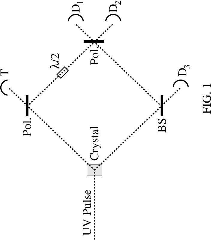
Figure 1: Scheme for the Innsbruck GHZ experiment. The GHZ correlations are obtained when all detectors $T,D_{1},D_{2},$ and $D3$ register a photon within the same window of time.

We will assume that double pairs created have the expected GHZ correlation, and the probability negligible of having triple pair produtions or of having fourfold coincidence registered when no photon is generated. (Our analysis is different from that of Żukowski [6], who considered only ideal detectors.) Two possibilities are left: i) a pair of photons is created at the parametric down converter; ii) two pairs of photons are created. We will denote by $p_{1}p_{2}$ the pair creation, and by $p_{1}...p_{4}$ the two-pair creation. We will assume that the probabilities add to one, i.e. $P\left(p_{1}\ldots p_{4}\right)+P\left(p_{1}p_{2}\right)=1.$

We start with two photons. $p_{1}p_{2}$ can reach any of the following combinations of detectors: $TD_{1},$ $TD_{2},$ $TD_{3},$ $D_{1}D_{1},$ $D_{1}D_{2},$ $D_{1}D_{3},$ $D_{2}D_{2},$ $D_{2}D_{3},$ $D_{3}D_{3},$ $TT$. For an event to be counted as being a GHZ state, all four detectors must fire (this conditionalization is equivalent to the enhancement hypothesis). We take as our set of random variables $\mathbf{T},\mathbf{D}_{1},\mathbf{D}_{2},\mathbf{D}_{3}$ which take values $1$ (if they fire) or $0$ (if they don’t fire). We will use $t,d_{1},d_{2},d_{3}$ ($\overline{t},\overline{d}_{1},\overline{d}_{2},\overline{d}_{3}$) to represent the value 1 (0). We want to compute $P\left(td_{1}d_{2}d_{3}\mid p_{1}p_{2}\right),$ the probability that all detectors $T,D_{1},D_{2},D_{3}$ fire simultaneously given that only a pair of photons has been created at the crystal. We start with the case when the two photons arrive at detectors $T$ and $D_{3}.$ Since the efficiency of the detectors is $d$, the probability that both detectors detect the photons is $d^{2},$ the probability that only one detects is $2d(1-d)$ and the probability that none of them detect is $(1-d)^{2}.$ Taking $\gamma$ into account, then the probability that all four detectors fire is

$$P\left(td_{1}d_{2}d_{3}\mid p_{1}p_{2}=TD_{3}\right)=\gamma^{2}\left(d+\gamma(1-d)\right)^{2},$$

where $p_{1}p_{2}=TD_{3}$ represents the simultaneous (i.e. within a measurement window) arrival of the photons a the trigger $T$ and at $D_{3}.$ Similar computations can be carried out for $p_{1}p_{2}=TD_{1},$ $TD_{2},$ $D_{1}D_{3},$ $D_{1}D_{2},$ $D_{2}D_{3}.$ For $p_{1}p_{2}=D_{i}D_{i}$ the computation of $P\left(td_{1}d_{2}d_{3}\mid p_{1}p_{2}=D_{i}D_{i}\right)$ is different. The probability that exactly one of the photons is detected at $D_{i}$ is $d(1-d)$ and the probability that none of them are detected is $(1-d)^{2}.$ Then, it is clear that

$$P\left(td_{1}d_{2}d_{3}\mid p_{1}p_{2}=D_{i}D_{i}\right)=d\left(1-d\right)\gamma^{3}+(1-d)^{2}\gamma^{4},$$

and we have at once that

$$P\left(td_{1}d_{2}d_{3}\mid p_{1}p_{2}\right) = 6\gamma^{2}\left(d+\gamma(1-d)\right)^{2}$$

$$+4\gamma^{3}\left(1-d\right)\left(d+\gamma\right).$$

We note that the events involving $P\left(td_{1}d_{2}d_{3}\mid p_{1}p_{2}\right)$ have no spin correlation, contrary to GHZ events.

We now turn to the case when four photons are created. The probability that all four are detected is $d^{4},$ that three are detected is $4d^{3}(1-d),$ that two are detected is $6d^{2}(1-d)^{2},$ that one is detected is $4d(1-d)^{3},$ and that none is detected is $(1-d)^{4}.$ If all four are detected, we have a true GHZ-correlated state detected. However, one can again have four detections due to dark counts. We will write $p_{1}...p_{4}=GHZ$ to represent having the four GHZ photons detected, and $p_{1}...p_{4}=\overline{GHZ}$ as having the four detections as a non-GHZ state. We can write that

$$P\left(td_{1}d_{2}d_{3}\mid p_{1}...p_{4}=GHZ\right)=d^{4}+\gamma\left(1-d\right)d^{3}$$ (5)

and

$$P\left(td_{1}d_{2}d_{3}\mid p_{1}...p_{4}=\overline{GHZ}\right)=3\gamma d^{3}(1-d)+6\gamma^{2}d^{2}(1-d)^{2}+4\gamma^{3}d(1-d)^{3}+\gamma^{4}(1-d)^{4}.$$

The last term in (5) comes from the unique role of the trigger $T,$ that needs to detect a photon but not necessarily one that has a GHZ correlation.

How do the non-GHZ detections change the GHZ expectations? What is measured in the laboratory is the conditional correlation $E\left(\mathbf{S}_{1}\mathbf{S}_{2}\mathbf{S}_{3}\mid td_{1}d_{2}d_{3}\right)$, where $\mathbf{S}_{1},$ $\mathbf{S}_{2}$ and $\mathbf{S}_{3}$ are random variables with values $\pm 1,$ representing the spin measurement at $D_{1},D_{2}$ and $D_{3}$ respectively. We can write it as

$$E\left(\mathbf{S}_{1}\mathbf{S}_{2}\mathbf{S}_{3}\mid td_{1}d_{2}d_{3}\right)=\frac{E\left(\mathbf{S}_{1}\mathbf{S}_{2}\mathbf{S}_{3}\mid td_{1}d_{2}d_{3}\,\,\&\,\,GHZ\right)P(GHZ)}{P(GHZ)+P(\overline{GHZ})}.$$

since for non-GHZ states we expect a correlation zero for the term

$$\frac{E\left(\mathbf{S}_{1}\mathbf{S}_{2}\mathbf{S}_{3}\mid td_{1}d_{2}d_{3}\,\,\&\overline{GHZ}\right)P(\overline{GHZ})}{P(GHZ)+P(\overline{GHZ})}.$$

Neglecting terms of higher order than $\gamma^{2}$, using $\gamma\ll d$, and $P(p_{1}p_{2})\gg P(p_{1}...p_{4}),$ we obtain, from $P(\overline{GHZ})=6P(p_{1}p_{2})\gamma^{2}d^{2}+3P(p_{1}...p_{4})\gamma(1-d)d^{3}$ and $P\left(GHZ\right)=P(p_{1}...p_{4})\left[d^{4}+\gamma\left(1-d\right)d^{3}\right],$ that

$$E\left(\mathbf{S}_{1}\mathbf{S}_{2}\mathbf{S}_{3}\mid td_{1}d_{2}d_{3}\right)=\frac{E(\mathbf{S}_{1}\mathbf{S}_{2}\mathbf{S}_{3}\mid td_{1}d_{2}d_{3}\&GHZ)}{\left[1+6\frac{P(p_{1}p_{2})}{P(p_{1}...p_{4})}\frac{\gamma^{2}}{d^{2}}\right]}.$$ (6)

This value is the corrected expression for the conditional correlations if we have detector efficiency taken into account. The product of the random variables $\mathbf{S}_{1}\mathbf{S}_{2}\mathbf{S}_{3}$ can take only values $+1$ or $-1.$ Then, if their expectation is $E\left(\mathbf{S}_{1}\mathbf{S}_{2}\mathbf{S}_{3}\mid td_{1}d_{2}d_{3}\right)$ we have

$$P\left(\mathbf{S}_{1}\mathbf{S}_{2}\mathbf{S}_{3}=1\mid td_{1}d_{2}d_{3}\right)=\frac{1+E\left(\mathbf{S}_{1}\mathbf{S}_{2}\mathbf{S}_{3}\mid td_{1}d_{2}d_{3}\right)}{2}.$$

The variance $\sigma^{2}$ for a random variable that assumes only $1$ or $-1$ values is $4P(1)\left(1-P(1)\right).$ Hence, in our case we have as a variance

$$\sigma^{2}=1-\left[E\left(\mathbf{S}_{1}\mathbf{S}_{2}\mathbf{S}_{3}\mid td_{1}d_{2}d_{3}\right)\right]^{2}.$$

We will estimate the values of $\gamma$ and $d$ to see how much $E\left(\mathbf{S}_{1}\mathbf{S}_{2}\mathbf{S}_{3}\mid td_{1}d_{2}d_{3}\right)$ would change due to experimental errors. For that purpose, we will use typical rates of detectors [7] for the frequency used at the Innsbruck experiment, as well as their reported data [5]. First, modern detectors usually have $d\cong 0.5$ for the wavelengths used at Innsbruck. We assume a dark-count rate of about $3\times 10^{2}$ counts/s. With a time window of coincidence measurement of $2\times 10^{-9}$ s, we then have that the probability of a dark count in this window is $\gamma\cong 6\times 10^{-7}.$ From [5] we use that the ratio $P(p_{1}p_{2})/P(p_{1}...p_{2})$ is on the order of $10^{10}.$ Substituting this three numerical values in (6) we have $E\left(\mathbf{S}_{1}\mathbf{S}_{2}\mathbf{S}_{3}\mid td_{1}d_{2}d_{3}\right)\cong 0.9.$ From this expression it is clear that the change in correlation imposed by the dark-count rates is significant for the given parameters. However, it is also clear that the value of the correlation is quite sensitive to changes in the values of both $\gamma$ and $d.$ We can now compare the values we obtained with the ones observed by Bouwmeester et al. for GHZ and $\overline{GHZ}$ states [5]. In their case, they claim to have obtained a ratio of $1:12$ between $\overline{GHZ}$ and GHZ states. In this case the correlations are $E\left(\mathbf{S}_{1}\mathbf{S}_{2}\mathbf{S}_{3}\mid td_{1}d_{2}d_{3}\right)\cong 0.92.$ It is clear that a detailed analysis of the parameters would be necessary to fit the experimental result to the predicted correlations that take the inefficiencies into account, but at this point one can see that values close to an experimentally measured $0.92$ can be obtained with appropriate choices of the parameters $d$ and $\gamma$ (see FIG. 2).

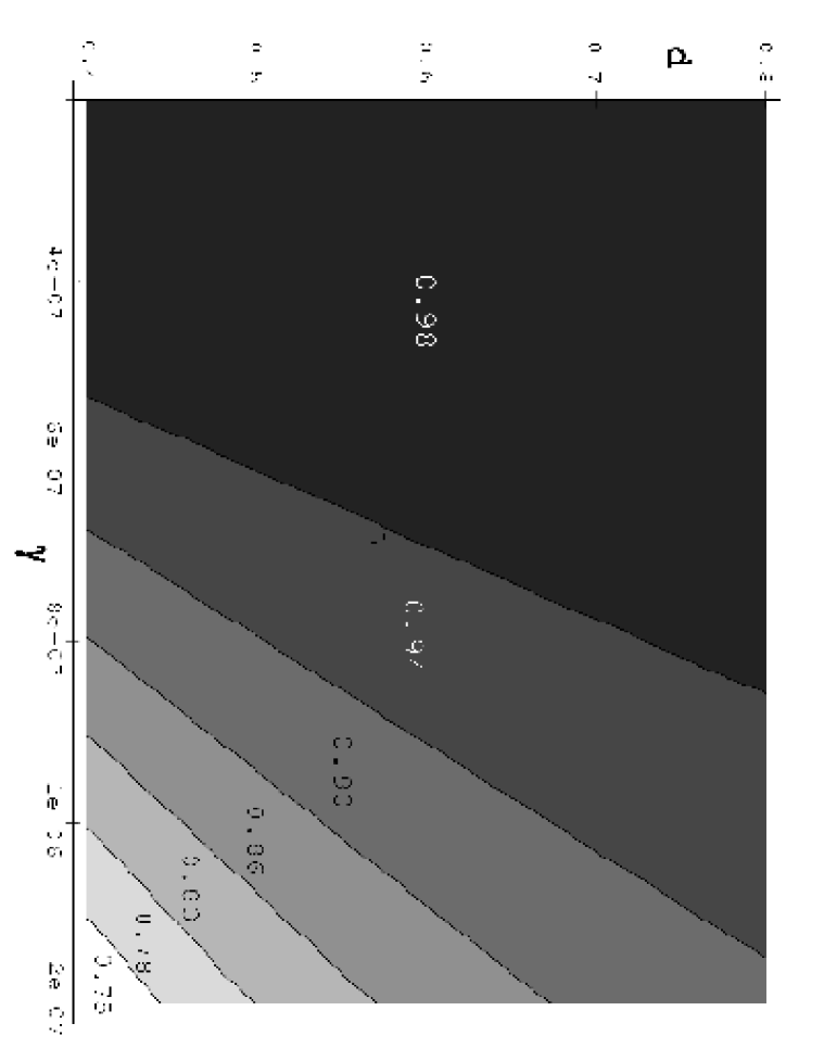
Figure 2: Contour plot of the correlation as a function of $\gamma$ and $d.$ The region where the correlation is $0.92$ defines a region for the parameters $\gamma$ and $d$ that is compatible with the Innsbruck results.

This expected correlation also satisfies

$$E\left(\mathbf{S}_{1}\mathbf{S}_{2}\mathbf{S}_{3}\mid td_{1}d_{2}d_{3}\right)>1-\frac{1}{2}.$$ (7)

This result is enough to prove the nonexistence of a joint probability distribution. We should note that the standard deviation in this case is

$$\sigma\cong\sqrt{\left(1+0.92\right)\left(1-0.92\right)}=0.39.$$ (8)

As a consequence, since $0.92-0.39=0.53,$ the result $0.92$ is bounded away from the classical limit $0.5$ by more than one standard deviation (see FIG. 3).

We showed that the GHZ theorem can be reformulated in a probabilistic way to include experimental inefficiencies. The set of four inequalities (1)-(4) sets lower bounds for the correlations that would prove the nonexistence of a local hidden-variable theory. Not surprisingly, detector inefficiencies and dark-count rates can change considerably the correlations. How do these results relate to previous ones obtained in the large literature of detector inefficiencies in experimental tests of local hidden-variable theories. We start with Mermin’s paper [9], where an inequality for $F$ similar to ours but for the case of $n$-correlated particles is derived. Mermin does not derive a minimum correlation for GHZ’s original setup that would imply the non-existence of a hidden-variable theory, as his main interest was to show that the quantum mechanical results diverge exponentially from a local hidden-variable theory if the number of entangled particles increase. Braunstein and Mann [8] take Mermin’s results and estimate possible experimental errors that were not considered here. They conclude that for a given efficiency of detectors the noise grows slower than the strong quantum mechanical correlations. Reid and Munru [10] obtained an inequality similar to our first one, but there are sets of expectations that satisfy their inequality and still do not have a joint probability distribution. In fact, as we mentioned earlier, our complete set of inequalities is a necessary and sufficient condition to have a joint probability distribution.

We have used an enhancement hypothesis, namely, that we only counted events with all four simultaneous detections, and showed that with the coincidence constraint a joint probability did not exist in the Innsbruck experiment. Enhancement hypotheses have to be used when detector efficiencies are low, but they may lead to loopholes in the arguments about the nonexistence of local hidden-variable theories. Loophole-free requirements for detector inefficiencies are based on the analysis of [11] for the Bell case and for [12] for the GHZ experiment without enhancement. However, in the Innsbruck setup enhancement is necessary, as the ratio of pair to two-pair production is of the order of $10^{10}$ [5]. Until experimental methods are found to eliminate the use of enhancement in GHZ experiments, no loophole-free results seem possible.

FIG. 3

Figure 3: Number of $\sigma$’s separating any observed correlation and the critical boundary 0.5. The square represents the reported correlation for the Innsbruck experiment, and the diamond represents the expected correlation if the dark count is reduced to 50 counts/s.

shows the number of standard deviations, as computed above, by which the existence of a joint distribution is violated. We can see that if we change the experiment such that we reduce the dark-count rate to 50 per second, instead of the assumed 300, a large improvement in the experimental result would be expected. Detectors with this dark-count rate and the assumed efficiency are available [7]. We emphasize that there are other possible experimental manipulations that would increase the observed correlation, e.g. the ratio $P(p_{1}p_{2})/P(p_{1}...p_{2}),$ but we cannot enter into such details here. The point to hold in mind is that FIG. 3 provides an analysis that can absorb any such changes or other sources of error, not just the dark-count rate, to give a measure of reliability.

We would like to thank Prof. Sebastião J. N. de Pádua for comments, as well as the anonymous referees.

References

[1]D. M. Greenberger, M. Horne, and A. Zeillinger, in Bell’s Theorem, Quantum
Theory, and Conceptions of the Universe, edited by M. Kafatos (Kluwer, Dordrecht,
1989).
[2]N. D. Mermin, Am. J. Phys.58, 731 (1990).
[3]J. F. Clauser, M. A. Horne, A. Shimony, and R. A. Holt, Phys. Rev. Lett. 23,
880 (1969).
[4]P. Suppes and M. Zanotti, Synthese48, 191 (1981).
[5]D. Bouwmeester, J-W. Pan, M. Daniell, H. Weingurter, and A. Zeilinger, Phys.
Rev. Lett.82, 1345 (1999).
[6]M. Żukowski, “Violation of Local Realism in the Innsbruck Experiment”,
quant-ph/9811013.
[7]Single photon count module specifications for EG&G’s SPCM-AG series were obtained
from EG&G’s web page at http://www.egginc.com.
[8]S. Braunstein and A. Mann, Phys. Rev.A47, R2427 (1993).
[9]N. D. Mermin, Phys. Rev. Lett.65, 1838 (1990).
[10]M. D. Reid and W. J. Munro, Phys. Rev. Lett.69, 997 (1992).