Adiabatic Output Coupling of a Bose Gas at Finite Temperatures

Abstract

We develop a general theory of adiabatic output coupling from trapped, weakly-interacting, atomic Bose-Einstein Condensates at finite temperatures. For weak coupling, the output rate from the condensate and the excited levels in the trap settles in a time proportional to the inverse of the spectral width of the coupling to the output modes. We discuss the properties of the output atoms in the quasi-steady-state where the population inside the trap is not appreciably depleted. We show how the composition of the output beam, containing the condensate and the thermal component, may be controlled by changing the frequency of the output coupling lasers. This composition determines the first and second order coherence of the output beam. We discuss the changes in the composition of the Bose gas left in the trap and show how non-resonant output coupling can stimulate either the evaporation of the thermal excitations in the trap or the growth of the non-thermal excitations, when pairs of correlated atoms leave the condensate.

I Introduction

Trapped atomic Bose-Einstein Condensates (BEC) are now routinely produced in various laboratories around the world, and it is important to understand the factors that influence the coherence of atoms transferred from them. This is an essential issue for the atom laser research, which has the long-term goal of producing continuous, directional, and coherent beams of atoms. A matter-wave pulse was first produced by using a radio frequency (RF) electromagnetic pulse to transfer atoms out of a trap, where they were allowed to fall freely under gravity[1, 2, 3]. More recently, a stimulated Raman process induced a transition to an untrapped magnetic state in an experiment at NIST; net momentum kick provided by the process resulted in a highly directional beam[4]. On the other hand, a long beam of atoms falling under gravity was produced in Munich using an RF-field-induced transition[5]. It is noted that although the more general features of the output in these experiments are fairly well-understood, detailed properties of the atoms in the output beam, and the evolution of the component that remains inside the trap have not so far been investigated.

Previous theoretical treatments of the output couplers for condensates have been either limited to a single-mode non-interacting trapped condensate[6, 7, 8] or to mean field treatment for the condensate[9, 10, 11, 12, 13, 14] which assume that the output beam is extracted out of a condensate at zero temperature and that they can be described by a single complex function of space and time. However, real condensates appear at finite temperatures, and as a result, thermal excitations play a major role.

In a previous paper[15], we outlined a theory of weak output coupling from a partially condensed, trapped Bose gas at finite temperatures. By applying the self-consistent Hartree-Fock-Bogoliubov (HFB) theory for Bose gases at finite temperatures, we identified three output components. The first is the output of pure condensates, which we have called “coherent output.” The second is the fraction emerging from the thermal excitations in the trap, which are coupled out of the trap by the process of “stimulated quantum evaporation.” This is equivalent to the quantum evaporation of Helium atoms from the surface of superfluid ⁴He, where phonon excitations travel up to the surface of the superfluid and then spontaneously emerge from the surface as evaporated atoms[16]. In our case such an evaporation from the trap is stimulated by an electromagnetic field. The last output component comes from the process of “pair breaking,” which involves simultaneous creation of an output coupled atom and an elementary excitation (quasi-particle) within the trap. For suitable choices of the coupling parameters each of the three processes can become the dominant process. We have shown that output coupling can serve not only as a useful way to extract an atomic beam out of a trap, but also as a probe to the delicate features of the quantum state of the Bose gas, including the pair correlations inside the condensate.

In this paper, we present an extensive analysis of the spectrum of the output atoms, and address issues that were not included in our shorter work. The first is the conditions for the output coupling to give a steady flow of atoms. We discuss the behaviour of the output rate and the atomic density in the short and the long time regimes, and also discuss the conditions for achieving a steady output beam. Second, the application of output coupling must cause changes in the state of the trapped Bose gas, such as changes of the number of excitations relative to the number of condensate atoms in the trap. We present a thorough discussion of these changes. The state of the Bose gas in the trap is usually described by the Bogoliubov formalism, which assumes an indefinite number of atoms in the system and therefore is not number-conserving. In this paper we discuss a number-conserving description of the system, which is especially useful when we consider the process of pair-breaking.

The results of this paper are directly applicable for any output coupling scheme which involves a single trapped state and one output state. We demonstrate here general fundamental issues by considering a one-dimensional Bose gas in a harmonic potential, which is coupled into a free output level in the absence of gravity.

The structure of this paper is as follows: We begin by deriving the equations of motion for the evolution of dynamical variables inside and outside the trap in Section II. We present in Section III a quasi-steady-state formalism, which enables us to obtain the properties of the output atoms. We demonstrate the results by a numerical example. We outline in Section IV the solution to the equations of motion in the trap that were derived in Section II, by introducing a number-conserving, time dependent Hartree-Fock-Bogoliubov (HFB) formulation in an adiabatic approximation. Applying this, we obtain expressions for the internal modes of the system in two different regimes, from which the time dependent quasiparticle excitations can be calculated. Finally, discussions and summary are given in Section V.

II The two-state output coupling model

In this section we present our model for describing the output coupling of a trapped Bose gas into free output modes. We derive the equations of motion for the atomic field operators in the trapped and the untrapped states, and give a general form of their solutions.

A Description of the model

Our model assumes that atoms are initially in an atomic magnetic level $|t\rangle$ (“the trapped state”) confined by a potential and in thermal equilibrium. A coupling interaction is then switched on, inducing transitions to a different magnetic level $|f\rangle$ (the “free” or “untrapped” state). We stress that these are labels denoting internal atomic levels, not the centre of mass states, so that for short enough times an atom in an $|f\rangle$ state may still be present within the trap. We use the atomic field operator $\hat{\psi}_{t}({\bf r})$ to describe the amplitude for the annihilation of a trapped atom at point ${\bf r}$, and the operator $\hat{\psi}_{f}({\bf r})$ to describe the corresponding amplitude for a free, untrapped atom. The Hamiltonian of the system takes the form

$$\hat{{\cal H}}=\hat{{\cal H}}_{t}^{(0)}+\hat{{\cal H}}_{f}^{(0)}+\hat{{\cal H}}_{\rm couple},$$ (1)

where $\hat{{\cal H}}_{t}^{(0)}$ and $\hat{{\cal H}}_{f}^{(0)}$ describe the dynamics of the trapped and untrapped atoms respectively while $\hat{{\cal H}}_{\rm couple}$ describes the coupling between the two states.

The dynamics inside the trap are given by the many-body Hamiltonian:

$$\hat{{\cal H}}_{t}^{(0)} = \int d^{3}{\bf r}\hat{\psi}_{t}^{{\dagger}}({\bf r})\left[-\frac{\hbar^{2}\nabla^{2}}{2m}+V_{t}({\bf r})\right]\hat{\psi}_{t}({\bf r})$$ (3)

$$+\frac{1}{2}\int d^{3}{\bf r}\int d^{3}{\bf r}^{\prime}\hat{\psi}_{t}^{{\dagger}}({\bf r})\hat{\psi}_{t}^{{\dagger}}({\bf r}^{\prime})U_{tt}({\bf r}-{\bf r}^{\prime})\hat{\psi}_{t}({\bf r}^{\prime})\hat{\psi}_{t}({\bf r}),$$

where $m$ is the mass of a single atom, $V_{t}({\bf r})$ is the potential responsible for the confinement of the atoms in the trap and $U_{tt}$ is the inter-particle potential between the trapped atoms.

With the output atoms, significant effect of their (elastic) collisions with the trapped atoms must be taken into account. In addition, we consider a small rate of output from the trap, so that the output atoms are dilute; this enables us to neglect the interactions between the free atoms themselves. Since the Bose gases are typically so dilute that their mean-free-path for the inelastic collisions is much larger than the dimensions of the atomic cloud in the trap, one may neglect also any inelastic collisions of the output atoms with the trapped atoms[17]. The Hamiltonian for the output atoms is then given by

$$\hat{{\cal H}}_{f}^{(0)} = \int d^{3}{\bf r}\hat{\psi}_{f}^{{\dagger}}({\bf r})\left[-\frac{\hbar^{2}\nabla^{2}}{2m}+V_{f}({\bf r})\right]\hat{\psi}_{f}({\bf r})$$ (5)

$$+\int d^{3}{\bf r}\int d^{3}{\bf r}^{\prime}\hat{\psi}_{f}^{{\dagger}}({\bf r})\hat{\psi}_{t}^{{\dagger}}({\bf r}^{\prime})U_{tf}({\bf r}-{\bf r}^{\prime})\hat{\psi}_{f}({\bf r}^{\prime})\hat{\psi}_{t}({\bf r}),$$

where $V_{f}({\bf r})$ is the potential that influences the propagation of the output free atoms and $U_{tf}$ is the collisional interaction between the trapped and free atoms; this is in general different from the interaction $U_{tt}$. We use the usual $\delta$-function form for the inter-particle potentials

$$U_{tt}({\bf r}-{\bf r}^{\prime}) = U_{0}\delta({\bf r}-{\bf r}^{\prime})$$ (6)

$$U_{tf}({\bf r}-{\bf r}^{\prime}) = U_{1}\delta({\bf r}-{\bf r}^{\prime}),$$ (7)

where $U_{0}=4\pi\hbar^{2}a_{tt}/m$ and $U_{1}=4\pi\hbar^{2}a_{tf}/m$ are proportional to the $s$-wave scattering lengths $a_{tt}$ and $a_{tf}$ for trapped-trapped and trapped-free collisions, respectively. We assume a repulsive interaction between the atoms, i.e. $U_{0,1}>0$.

For the Hamiltonian $\hat{{\cal H}}_{\rm couple}$, we consider coupling by an electromagnetic (EM) field which induces transitions between the states $|t\rangle$ and $|f\rangle$. In the rotating wave approximation, the EM coupling mechanism may be described by the following Hamiltonian, which can quite clearly be generalised to describe any kind of linear coupling such as weak tunnelling:

$$\hat{{\cal H}}_{\rm couple}=\hbar\int d^{3}{\bf r}\lambda({\bf r},t)\hat{\psi}_{f}^{{\dagger}}({\bf r})\hat{\psi}_{t}({\bf r})+h.c.$$ (8)

Here $\lambda({\bf r},t)$ denotes the amplitude of coupling between the trapped and the untrapped magnetic states. The form of $\lambda({\bf r},t)$ depends on the type of coupling used: Typical mechanisms are direct (one-photon) radio-frequency transition and indirect (two-photon) stimulated Raman transition. For any EM induced processes, the coupling can be written as

$$\lambda({\bf r},t)=\bar{\lambda}({\bf r},t)e^{i({\bf k}_{\rm em}\cdot{\bf r}-\Delta_{em}t)},$$ (9)

where $\bar{\lambda}$ is slowly varying in space and time. $\bar{\lambda}$ can be either time-independent, to describe a continuous electromagnetic wave, or pulsed. $\hbar{\bf k}_{\rm em}$ and $\hbar\Delta_{\rm em}$ measure the net momentum and energy transfer from the EM field to an output atom. In an RF coupling scheme, $\bar{\lambda}({\bf r},t)$ is the Rabi frequency $\Omega({\bf r},t)=\langle\hat{p}\rangle{\cal E}({\bf r},t)/\hbar$ (or $\langle\hat{\mu}\rangle{\cal B}({\bf r},t)/\hbar$) corresponding to the flipping of the atomic electric (or magnetic) dipole $\langle\hat{p}\rangle$ (or $\langle\hat{\mu}\rangle$) in the electric (or magnetic) field ${\cal E}({\bf r},t)$ (${\cal B}({\bf r},t)$); $\Delta_{\rm em}$ is the detuning of the EM field frequency from the transition frequency and ${\bf k}_{\rm em}$ is, in general, negligible compared to the initial momentum distribution of the atoms. In the stimulated Raman coupling, two laser beams are used to induce a transition from $|t\rangle$ to $|f\rangle$ through an intermediate level $|i\rangle$, and

$$\bar{\lambda}({\bf r},t)=\frac{\Omega^{*}_{ti}({\bf r},t)\Omega_{fi}({\bf r},t)}{\Delta_{i}},$$ (10)

where $\Omega_{ti}$ and $\Omega_{fi}$ are the Rabi frequencies corresponding to the intermediate transitions and $\Delta_{i}$ is their detuning from resonance with the two beams. $\Delta_{\rm em}$ and ${\bf k}_{\rm em}$ are the differences between the frequencies and momenta associated with the two laser beams:

$$\Delta_{em} = \omega_{1L}-\omega_{2L}-\frac{E_{t}^{(0)}-E_{f}^{(0)}}{\hbar},$$ (11)

$${\bf k}_{em} = {\bf k}_{1L}-{\bf k}_{2L},$$ (12)

where $E_{t}^{(0)}-E_{f}^{(0)}$ is the energy splitting between the atomic levels $|t\rangle$ and $|f\rangle$ in the centre of the trap. A more detailed derivation of Eq. (10) for the Raman process is provided in Appendix A. An energy level diagram depicting the output coupling through the stimulated Raman process is given in Fig. 1.

B Equations of motion

The coupled equations of motion for the trapped and free field operators are obtained by computing their commutation relations with the Hamiltonian (1). We thus find

$$\frac{\partial}{\partial t}\hat{\psi}_{t}({\bf r},t) = -\frac{i}{\hbar}{\cal L}_{t}\hat{\psi}_{t}({\bf r},t)-\frac{i}{\hbar}U_{0}\hat{\psi}_{t}^{{\dagger}}({\bf r},t)\hat{\psi}_{t}({\bf r},t)\hat{\psi}_{t}({\bf r},t)$$ (14)

$$-i\lambda^{*}({\bf r},t)\hat{\psi}_{f}({\bf r},t),$$

$$\frac{\partial}{\partial t}{\hat{\psi}}_{f}({\bf r},t) = -\frac{i}{\hbar}{\cal L}_{f}\hat{\psi}_{f}({\bf r},t)-i\lambda({\bf r},t)\hat{\psi}_{t}({\bf r},t),$$ (15)

where

$${\cal L}_{t} \equiv -\hbar^{2}\nabla^{2}/2m+V_{t}({\bf r}),$$ (16)

$${\cal L}_{f} \equiv -\hbar^{2}\nabla^{2}/2m+V_{f}({\bf r})+U_{1}\langle\hat{\psi}_{t}^{{\dagger}}({\bf r})\hat{\psi}_{t}({\bf r})\rangle.$$ (17)

In Eq. (17) we have used a mean-field approximation for the collisional effect of the trapped atoms on the untrapped ones. This approximation neglects inelastic scattering processes with the trapped atoms[17] and other possible effects of entanglement of the output atoms with the atoms in the trap. The approximation is justified under the assumption of long atomic mean-free-path mentioned above.

C General solutions

1 Output atoms

The formal solution of Eq. (15) for $\hat{\psi}_{f}$ in terms of $\hat{\psi}_{t}$ is

$$\hat{\psi}_{f}({\bf r},t)=\hat{\psi}_{f}^{(0)}({\bf r},t)-i\int_{0}^{t}dt^{\prime}\int d^{3}{\bf r}^{\prime}K_{f}({\bf r},{\bf r}^{\prime},t-t^{\prime})\lambda({\bf r}^{\prime},t^{\prime})\hat{\psi}_{t}({\bf r}^{\prime},t^{\prime}),$$ (18)

where $\hat{\psi}_{f}^{(0)}$ satisfies the time-dependent Schrödinger equation for the free evolution of $\hat{\psi}_{f}$ in the absence of output coupling

$$\frac{\partial}{\partial t}\hat{\psi}_{f}^{(0)}=-\frac{i}{\hbar}{\cal L}_{f}\hat{\psi}_{f}^{(0)},$$ (19)

and the “free” propagator $K_{f}({\bf r},{\bf r}^{\prime},t-t^{\prime})$ satisfies the partial differential equation

$$\frac{\partial}{\partial t}K_{f}({\bf r},{\bf r}^{\prime},t-t^{\prime})=-\frac{i}{\hbar}{\cal L}_{f}K_{f}({\bf r},{\bf r}^{\prime},t-t^{\prime})+\delta({\bf r}-{\bf r}^{\prime})\delta(t-t^{\prime}).$$ (20)

The second term in Eq. (18) describes the transition of the atoms from the trapped level $|t\rangle$ into the free level $|f\rangle$ with amplitude $\lambda({\bf r},t)$ and their subsequent propagation as free atoms.

We note that it is useful to expand the field operator $\hat{\psi}_{f}$ in terms of the normal modes $\varphi_{{\bf k}}({\bf r})$ of the untrapped level

$$\hat{\psi}_{f}({\bf r},t)=\sum_{{\bf k}}\varphi_{{\bf k}}({\bf r})\hat{b}_{{\bf k}}(t),$$ (21)

where $\hat{b}_{{\bf k}}$ satisfy the usual bosonic commutation relations $[\hat{b}_{{\bf k}},\hat{b}_{{\bf k}^{\prime}}^{{\dagger}}]=\delta_{{\bf k},{\bf k}^{\prime}}$. ${\bf k}$ denotes the momentum state of the free atoms with energy $E_{{\bf k}}=\hbar\omega_{{\bf k}}$, and $\varphi_{{\bf k}}$ are the time-independent solutions of the single-particle problem in the non-trapping effective potential $V_{f}({\bf r})+U_{1}\langle\hat{\psi}_{t}^{{\dagger}}({\bf r})\hat{\psi}_{t}({\bf r})\rangle$ created by the mean field effect of the collisions between the trapped and the free atoms. In principle, the solutions $\varphi_{{\bf k}}$ and the energies $E_{{\bf k}}$ may change with time due to the change in the density of the trapped atoms and the subsequent change in the effective repulsive potential near the trap. In what follows we will neglect this time-dependence under the assumption of weak output coupling and slow changes in the density of the trapped atoms.

In the absence of gravitational or other forces, at positions far away from the trap, ${\bf k}$ may be taken to be the wave number of a plane wave $\varphi_{{\bf k}}\sim e^{i{\bf k}\cdot{\bf r}}$ with $\omega_{{\bf k}}=\hbar k^{2}/2m$. In the presence of gravity, the structure of the output modes should be defined appropriately, and the modes ${\bf k}$ may be given asymptotically by the solutions of the Schrödinger equation in a homogeneous field. In Eq. (21) we have used a sum $\sum_{{\bf k}}$ over discrete output states. It is noted that the actual structure of the Hilbert space for the output modes depends on the potential $V_{f}({\bf r})$; if this potential vanishes far away from the centre of the trap, then the sum $\sum_{{\bf k}}$ should be replaced by an integral $\int d^{3}{\bf k}$ and the operators $\hat{b}_{{\bf k}}$ should be defined such that $[\hat{b}_{{\bf k}},\hat{b}^{{\dagger}}_{{\bf k}^{\prime}}]=\delta({\bf k}-{\bf k}^{\prime})$.

In terms of the basis functions $\varphi_{{\bf k}}({\bf r})$, the free field operator $\hat{\psi}_{f}^{(0)}$ is given by

$$\hat{\psi}_{f}^{(0)}({\bf r},t)=\sum_{{\bf k}}\varphi_{{\bf k}}({\bf r})\hat{b}_{{\bf k}}(0)e^{-i\omega_{{\bf k}}t}$$ (22)

and the propagator of the free atoms may be written as

$$K_{f}({\bf r},{\bf r}^{\prime},t-t^{\prime})=\sum_{{\bf k}}\varphi_{{\bf k}}({\bf r})\varphi^{*}_{{\bf k}}({\bf r}^{\prime})e^{-i\omega_{{\bf k}}(t-t^{\prime})}\theta(t-t^{\prime}).$$ (23)

It is useful to describe the evolution of the untrapped atoms in terms of the annihilation operators $\hat{b}_{{\bf k}}$ in a specific mode ${\bf k}$. The solution for this operator is obtained by multiplying Eq. (18) by $\varphi^{*}_{{\bf k}}$ and integrating over all space:

$$\hat{b}_{{\bf k}}(t)=\hat{b}_{{\bf k}}(0)e^{-i\omega_{{\bf k}}t}-i\int_{0}^{t}dt^{\prime}\int d^{3}{\bf r}\varphi^{*}_{{\bf k}}({\bf r})\lambda({\bf r},t^{\prime})e^{-i\omega_{{\bf k}}(t-t^{\prime})}\hat{\psi}_{t}({\bf r},t^{\prime}).$$ (24)

Solutions for the output field $\hat{\psi}_{t}({\bf r},t)$ in Eqs. (18) and (24) require an explicit expression for the trapped field operator $\hat{\psi}_{t}({\bf r},t^{\prime})$. The simplest approximation is to take the first order solution in the coupling amplitude $\lambda({\bf r},t)$. This corresponds to a very weak coupling and $\hat{\psi}_{t}({\bf r},t)\approx\hat{\psi}_{t}^{(0)}({\bf r},t)$, where $\hat{\psi}_{t}^{(0)}({\bf r},t)$ is the field operator of the trapped atoms without output coupling. The fundamental properties of the output under such approximation will be the main subject of Sec. III.

2 Trapped atoms

By substituting the solution (18) for $\hat{\psi}_{f}$ back into Eq. (14) we obtain the following equation for the trapped field operator $\hat{\psi}_{t}({\bf r},t)$

$$\frac{\partial}{\partial t}\hat{\psi}_{t}({\bf r},t) = -\frac{i}{\hbar}{\cal L}_{t}\hat{\psi}_{t}({\bf r},t)-\frac{i}{\hbar}U_{0}\hat{\psi}_{t}^{{\dagger}}({\bf r},t)\hat{\psi}_{t}({\bf r},t)\hat{\psi}_{t}({\bf r},t)$$ (26)

$$-\int_{0}^{t}dt^{\prime}\int d^{3}{\bf r}G({\bf r},{\bf r}^{\prime},t,t^{\prime})\psi_{t}({\bf r}^{\prime},t^{\prime})-i\lambda^{*}({\bf r},t)\hat{\psi}_{f}^{(0)}({\bf r},t),$$

where

$$G({\bf r},{\bf r}^{\prime},t,t^{\prime})=\lambda^{*}({\bf r},t)K_{f}({\bf r},{\bf r}^{\prime},t-t^{\prime})\lambda({\bf r}^{\prime},t^{\prime}).$$ (27)

The solution of the integro-differential equation, Eq. (26) will be the main subject of Sec. IV. In principle, two different situations may be expected from such an integro-differential equation. In the case where this equation describes a coupling to the output levels with a narrow available bandwidth compared to the coupling strength $\lambda({\bf r},t)$, we anticipate Rabi oscillations of the atomic population between the trapped and untrapped levels. Physically, this means that the output atoms stay near the trap for a long enough time to perform these oscillations. On the other hand, when the bandwidth of the output modes is large compared to the coupling strength, an exponential decay of the population in the trap is expected. Physically, this behaviour is expected when the output atoms are fast enough to escape from the trap before the interaction couples them back into the trapped level. Even if the coupling is very weak, an oscillatory kind of behaviour is expected for short times compared to the inverse of the bandwidth of the relevant output modes, before the output rate settles on a constant rate with fixed energy. For this last case, Eq. (26) may be viewed as a Langevin equation for an interaction of a confined system with an infinite heat bath[12].

The trapped field operators $\hat{\psi}_{t}({\bf r},t)$ can, in principle, be expanded similarly to the field operator $\hat{\psi}_{f}({\bf r},t)$ as

$$\hat{\psi}_{t}({\bf r},t)=\sum_{n}\phi_{n}({\bf r})\hat{a}_{n}(t),$$ (28)

where $\phi_{n}({\bf r})$ are the normal modes of the trap given by the solutions of the single-particle problem in the potential well $V_{t}({\bf r})$. These eigenmodes, however, do not form a good basis, since the interaction between the atoms results in a strong mixing between the levels. In the following sections, therefore, we will instead use the basis of condensate and its quasi-particle excitations, which are obtained from the Hartree-Fock-Bogoliubov theory of an interacting Bose gas.

III Output properties in the quasi-steady state

In this section we present the properties of the output atoms under the assumption that the output coupling is very weak. In this case, the output beam of atoms can serve as a probe to the structure of the Bose gas in the trap under steady-state conditions. The solution for the output is given by Eq. (18), or equivalently Eq. (24), where we substitute $\hat{\psi}_{t}({\bf r},t)\approx\hat{\psi}_{t}^{(0)}({\bf r},t)$. We start this section by giving a brief description of the formalism that allows the use of the steady-state solution $\hat{\psi}_{t}^{(0)}({\bf r},t)$ for the atoms in the trap. We then present basic properties of the output, in particular the spectrum and the density of the output coupled atoms. Finally the first and second order correlations of the output atoms are presented.

A The trapped atoms in the quasi steady-state

We briefly review in this subsection the theory of the trapped Bose gas in steady-state conditions, in a way that will enable us in Sec. IV to extend the theory to the time-dependent case where the number of atoms in the trap does change adiabatically during output coupling. Since the situations discussed in this paper involve transitions of atoms into untrapped propagating states where counting the number of output atoms could be one of the main measurements, we choose to use a number-conserving theory in the spirit of the theories put forward recently[20]. In addition, the theory enables an extension of the finite temperature HFB-Popov method into time dependent cases.

For describing a partially condensed system of atoms at a finite temperature, we split the field operator for the atoms in the trap into a part which is proportional to the condensate wave function and a part which represents excitations orthogonal to this state:

$$\hat{\psi}_{t}({\bf r},t)=e^{-i\Phi(t)}\left[\psi_{0}({\bf r})\hat{a}_{0}(t)+\delta\hat{\psi}({\bf r},t)\right].$$ (29)

Here $\Phi(t)$ is a global phase given by

$$\Phi(t)=\int^{t}_{0}\mu(t^{\prime})dt^{\prime},$$ (30)

where $\mu$, the chemical potential of the system for the given global variables, is constant under steady-state conditions. The operator $\hat{a}_{0}$ is a bosonic annihilation operator satisfying $[\hat{a}_{0},\hat{a}_{0}^{{\dagger}}]=1$ and describes the annihilation of one atom in the condensate state $\psi_{0}({\bf r})$. The number of condensate atoms is represented by the operator $\hat{N}_{0}\equiv\hat{a}_{0}^{{\dagger}}\hat{a}_{0}$. The non-condensate part, $\delta\hat{\psi}$, is assumed to be orthogonal to the condensate in the sense $\int d^{3}{\bf r}\hat{\psi}^{*}_{0}({\bf r},t)\delta\hat{\psi}({\bf r},t)=0$. In the number conserving formalism $\delta\hat{\psi}$ is approximated by the following Bogoliubov form:

$$\delta\hat{\psi}({\bf r},t)\approx\hat{a}_{0}\frac{1}{\sqrt{\hat{N}_{0}}}\sum_{j}[u_{j}({\bf r})\hat{\alpha}_{j}(t)+v^{*}_{j}({\bf r})\hat{\alpha}^{{\dagger}}_{j}(t)],$$ (31)

where $\hat{\alpha}_{j},\hat{\alpha}^{{\dagger}}_{j}$ are the bosonic operators satisfying $[\hat{\alpha}_{i},\hat{\alpha}_{j}^{{\dagger}}]=\delta_{ij}$ in the space of states with non-zero condensate number, and they describe the annihilation or creation of excitations (quasi-particles), or, equivalently, transitions from an excited state $j$ into the condensate and vice versa. This implies that the operators $\hat{\alpha}_{j},\hat{\alpha}_{j}^{{\dagger}}$ do not commute with the condensate operator $\hat{a}_{0}$. The wave functions $u_{j}({\bf r})$ and $v_{j}({\bf r})$ are the corresponding amplitudes associated with the annihilation of a real particle at position ${\bf r}$, an action which involves both annihilation or creation of excitations on top of the condensate. The time-dependence of the functions $\psi_{0},u_{j},v_{j}$ is induced only by the change in the global variables $V_{t}({\bf r},t),N_{t}(t),E_{trap}(t)$ and they are assumed to be time-independent under the steady-state conditions.

The condensate wave function $\psi_{0}({\bf r})$ in Eq. (29) is defined as the solution of the generalised steady-state Gross-Pitaevskii equation

$$\{{\cal L}_{t}-\mu+U_{0}[\bar{N}_{0}|\psi_{0}({\bf r})|^{2}+2\bar{n}({\bf r})]\}\psi_{0}({\bf r})=0$$ (32)

where ${\cal L}_{t}$ is given in Eq. (16), while the adiabatic mean number $\bar{N}_{0}$ of the condensate atoms and the density $\bar{n}({\bf r})$ of the non-condensate atoms are calculated self-consistently by requiring

$$\bar{N}_{0}+\int d^{3}{\bf r}\bar{n}({\bf r})=N_{t}.$$ (33)

The functions $u_{j}({\bf r}),v_{j}({\bf r})$ satisfy the steady-state equations

$$\left(\begin{array}[]{cc}{\cal L}_{t}-\mu+2U_{0}[\bar{N}_{0}|\psi_{0}({\bf r})|^{2}+\bar{n}({\bf r})]&U_{0}\bar{N}_{0}(\psi_{0}({\bf r}))^{2}\\ -U_{0}\bar{N}_{0}(\psi_{0}^{*}({\bf r}))^{2}&-{\cal L}_{t}+\mu-2U_{0}[\bar{N}_{0}|\psi_{0}({\bf r})|^{2}+\bar{n}({\bf r})]\end{array}\right)\left(\begin{array}[]{c}u_{j}({\bf r})\\ v_{j}({\bf r})\end{array}\right)=E_{j}\left(\begin{array}[]{c}u_{j}({\bf r})\\ v_{j}({\bf r})\end{array}\right)$$ (40)

$$+U_{0}\bar{N}_{0}\int d^{3}{\bf r}|\psi_{0}({\bf r})|^{2}[\psi^{*}_{0}({\bf r})u_{j}({\bf r})+\psi_{0}({\bf r})v_{j}({\bf r})]\left(\begin{array}[]{c}\psi_{0}({\bf r})\\ \psi^{*}_{0}({\bf r})\end{array}\right),$$ (43)

where $E_{j}=\hbar\omega_{j}$ are the $j$th quasi-particle excitation energy with respect to the condensate ground state energy, and the second term on the right hand side ensures the orthogonality of the non-condensate functions with the condensate[21]. We note that the vectors $\left(\begin{array}[]{c}v^{*}_{j}\\ u^{*}_{j}\end{array}\right)$ satisfy an equation similar to Eq. (43) with $E_{j}\rightarrow-E_{j}$; Eqs. (32) and (43) must be solved self-consistently for any given global conditions. The mean number of atoms in an excited state in equilibrium is assumed to be given by the Bose-Einstein distribution

$$n^{eq}_{j}=\frac{1}{\exp[\hbar\omega_{j}/T]-1}.$$ (44)

In this section we assume a weak output process so that the total number of atoms in the trap does not change significantly during the application of the output coupling. Under these conditions the time-dependence of the operators $\hat{a}_{0}$ and $\hat{\alpha}_{j}$ is assumed to be simply

$$\hat{a}_{0}(t) \approx \hat{a}_{0}(0)$$ (45)

$$\hat{\alpha}_{j}(t) \approx \hat{\alpha}_{j}(0)e^{-i\omega_{j}t}.$$ (46)

In our numerical demonstration throughout this paper we take a one dimensional Bose gas of $N_{t}=2000$ atoms in a harmonic trap with frequency $\omega$. The critical temperature for condensation in this case is $T_{c}\sim 300\hbar\omega/k$. We have used a self-consistent HFB-Popov method to find the wave functions and energies of the condensate and the excitations. Throughout this paper we take $U_{0}=10\hbar\omega\sqrt{2\hbar/m\omega}$. We present calculations for two temperatures: for $T=10\hbar\omega/k$ we obtain the chemical potential $\mu\approx 2.5\hbar\omega$ and the non-condensate fraction $\sim 2\%$. At $T=150\hbar\omega/k$ we obtain $\mu\approx 2.3\hbar\omega/k$ and the non-condensate fraction is $\sim 44\%$. We take the interaction strength between the trapped and untrapped atoms to be $U_{1}=U_{0}$. Length will be presented in units of $2\sqrt{\hbar/m\omega}$ (“harmonic-oscillator units”).

B Basic properties of the output

In order to obtain the properties of the output we expand the output field operator $\hat{\psi}_{f}$ in terms of the free modes $\varphi_{{\bf k}}$ in the quasi-steady-state[Eq. (21)]. We assume $\lambda({\bf r},t)=\lambda({\bf r})e^{-i\Delta_{em}t}$. Using the form (29) and (31) of $\hat{\psi}_{t}$ and the assumptions (45) and (46), we obtain from Eq. (24) the following equation for the annihilation operators of the free output modes

$$\hat{b}_{{\bf k}}(t) \approx e^{-i\omega_{{\bf k}}t}\left\{\hat{b}_{{\bf k}}(0)-i\left\{\lambda_{{\bf k}0}D_{{\bf k}0}(t)\hat{a}_{0}(0)\right.\right.$$ (48)

$$\left.\left.+\hat{a}_{0}\frac{1}{\sqrt{\hat{N}_{0}}}\sum_{j}[\lambda_{{\bf k}j+}D_{{\bf k}j+}(t)\hat{\alpha}_{j}(0)+\lambda_{{\bf k}j-}D_{{\bf k}j-}(t)\hat{\alpha}^{{\dagger}}_{j}(0)]\right\}\right\},$$

where

$$\lambda_{{\bf k}0} = \int d^{3}{\bf r}\varphi_{{\bf k}}^{*}({\bf r})\lambda({\bf r})\psi_{0}({\bf r})$$ (49)

$$\lambda_{{\bf k}j+} = \int d^{3}{\bf r}\varphi_{{\bf k}}^{*}({\bf r})\lambda({\bf r})u_{j}({\bf r})$$ (50)

$$\lambda_{{\bf k}j-} = \int d^{3}{\bf r}\varphi_{{\bf k}}^{*}({\bf r})\lambda({\bf r})v^{*}_{j}({\bf r})$$ (51)

are the matrix elements of $\lambda({\bf r})$ between the wave functions of the collective excitations and the output states. The time- and energy- dependence is determined by the functions

$$D_{{\bf k}\eta}(t)=i\frac{e^{-i(\omega_{out}^{\eta}-\omega_{{\bf k}})t}-1}{\omega_{out}^{\eta}-\omega_{{\bf k}}},$$ (52)

where

$$\hbar\omega_{out}^{\eta}=\mu+\Delta_{em}+E_{\eta},$$ (53)

with $\eta=0,j+,j-$, and $E_{j+}=E_{j}$ and $E_{j-}=-E_{j}$.

With the above definitions, the field operator $\hat{\psi}_{f}({\bf r},t)$ of the free atoms can be written as

$$\hat{\psi}_{f}({\bf r},t) \approx \hat{\psi}_{f}^{(0)}({\bf r},t)-i\Psi_{f}^{0}({\bf r},t)\hat{a}_{0}(0)$$ (55)

$$-\hat{a}_{0}(0)\frac{i}{\sqrt{\hat{N}_{0}}}\sum_{j}\left[\Psi_{f}^{j+}({\bf r},t)\hat{\alpha}_{j}(0)+\Psi_{f}^{j-}({\bf r},t)\hat{\alpha}^{{\dagger}}_{j}(0)\right],$$

where

$$\Psi_{f}^{\eta}({\bf r},t)=\sum_{{\bf k}}\varphi_{{\bf k}}({\bf r})D_{{\bf k}\eta}(t)\lambda_{{\bf k}\eta}e^{-i\omega_{{\bf k}}t}$$ (56)

for each $\eta=0,j+,j-$.

This result enables us to calculate various properties of the output from the trap, assuming Bose-Einstein statistics for the initial quasiparticle populations inside the trap. For the initial state we assume that all the cross correlation functions between different operators $\hat{a}_{0},\hat{\alpha}_{j},\hat{\alpha}_{j}^{{\dagger}}$ vanish, and the only non-zero contributions are the populations

$$\langle\hat{a}_{0}^{{\dagger}}\hat{a}_{0}\rangle=N_{0}\equiv n_{0}^{t}$$ (57)

$$\langle\hat{\alpha}^{{\dagger}}_{j}\hat{\alpha}_{j}\rangle=n_{j}\equiv n^{t}_{j+}$$ (58)

$$\langle\hat{\alpha}_{j}\hat{\alpha}^{{\dagger}}_{j}\rangle=n_{j}+1\equiv n^{t}_{j-}.$$ (59)

Any measurable quantities related to the output atoms may be expressed in terms of the correlation functions of the field operator $\hat{\psi}_{f}({\bf r},t)$ at different times and space points. In particular, the density of output atoms at a given point ${\bf r}$ and time $t$ is given by the equal-time, equal-position correlation function

$$n_{out}({\bf r},t)=\langle\hat{\psi}_{f}^{{\dagger}}({\bf r},t)\hat{\psi}_{f}({\bf r},t)\rangle.$$ (60)

By using Eq. (55) and the assumptions (57)-(59) we observe that $n_{out}({\bf r},t)$ can be written as a sum over discrete contributions from the levels in the trap

$$n_{out}({\bf r},t)=N_{0}|\Psi^{0}_{f}({\bf r},t)|^{2}+\sum_{j}\left[n_{j}|\Psi^{j+}_{f}({\bf r},t)|^{2}+(n_{j}+1)|\Psi^{j-}_{f}({\bf r},t)|^{2}\right],$$ (61)

where the first term is the condensate output, the second term is the contribution from the stimulated quantum evaporation of the thermal excitations, and the third term is the contribution from the pair-breaking process, as discussed in Ref. [15].

Following similar steps, the number of output atoms in mode ${\bf k}$ of the free atomic level, $n_{{\bf k}}\equiv\langle\hat{b}_{{\bf k}}^{{\dagger}}\hat{b}_{{\bf k}}\rangle$, is given by a sum of discrete contributions from the different levels of the trapped gas

$$n_{{\bf k}}(t)=n_{{\bf k}}^{0}(t)+\sum_{j}\left[n_{{\bf k}}^{j+}(t)+n_{{\bf k}}^{j-}(t)\right],$$ (62)

where each term $\eta=0,j+,j-$ in Eq. (62) has the form

$$n_{{\bf k}}^{\eta}(t)=|\lambda_{{\bf k}\eta}|^{2}|D_{{\bf k}\eta}(t)|^{2}n^{t}_{\eta}.$$ (63)

The time- and energy- dependence of each of the $n_{{\bf k}}^{\eta}$ is given by the function

$$|D_{{\bf k}\eta}(t)|^{2}=\frac{1}{2}\left[\frac{\sin[(\omega_{{\bf k}}-\omega_{out}^{\eta})t/2]}{(\omega_{{\bf k}}-\omega_{out}^{\eta})/2}\right]^{2}.$$ (64)

This function has a spectral width in $\omega_{\bf k}$ which decreases with time as $\sim\pi/t$. This spectral width represents the energy uncertainty dictated by the finite duration of the output coupling process. The time evolution of the output atoms is therefore governed by the spectral dependence of the matrix elements $\lambda_{{\bf k}\eta}$.

In order to analyse the evolution of the output rate and the output atom density, we define two frequency scales with regard to the matrix elements $\lambda_{{\bf k}\eta}$ for each $\eta=0,j+,j-$: (1) $\Delta\omega_{\eta}$, the frequency bandwidth within which the matrix elements $\lambda_{{\bf k}\eta}$, defined in Eqs. (49)-(51), are significant and (2) $\delta\omega_{\eta}$, the “width” of $\lambda_{{\bf k}\eta}$ in the $\omega_{{\bf k}}\equiv\hbar k^{2}/2m$ space in the vicinity of $\omega_{{\bf k}}=\omega_{out}^{\eta}$. The weak coupling assumption is justified if the strength of the coupling, which may be represented by the parameter $\Lambda=\sqrt{\int d^{3}{\bf r}|\lambda({\bf r})|^{2}}$ is much smaller than $\Delta\omega_{\eta}$ of each trap state, namely,

$$\Lambda\ll\Delta\omega_{\eta}.$$ (65)

If this condition is not satisfied, then we expect Rabi oscillations between the trapped atomic level $|t\rangle$ and the output level $|f\rangle$[22]. In the case of weak coupling, we may identify three temporal regimes:

1. Very short times, $t\ll\Delta\omega_{\eta}^{-1}$. Then the function $D_{{\bf k}\eta}(t)$ in Eq. (52) becomes independent of ${\bf k}$, and if $\omega_{out}^{\eta}$ lies within the bandwidth $\Delta\omega_{\eta}$, $D_{{\bf k}\eta}(t)\approx t$. In this case, the completeness of the set of functions $\varphi_{{\bf k}}({\bf r})$ implies

   $$\Psi_{f}^{\eta}({\bf r},t)\sim_{t\rightarrow 0}\lambda({\bf r})\psi_{t}^{\eta}({\bf r})t,$$ (66)

   where $\psi_{t}^{0}=\psi_{0},\psi_{t}^{j+}=u_{j}$, and $\psi_{t}^{j-}=v_{j}^{*}$. The initial shape of the output wave functions before it had time to propagate is therefore the overlap of the electromagnetic field amplitude and the corresponding trapped wave function. The density $n_{out}({\bf r})$ in this case is then similar in shape to the density of atoms in the trap and the total number of output atoms increases quadratically in time. This result may also be used to calculate the output beam immediately after the application of a strong coupling pulse, before the output beam starts to propagate or Rabi oscillations occur.

2. Intermediate times, $\Delta\omega_{\eta}^{-1}<t<\delta\omega_{\eta}^{-1}$. In this case the rate of output from each trap state $\eta$ may show oscillations, which follow from interference between output from different momentum states.

3. Long times, $t\gg\delta\omega_{\eta}^{-1}$. The output from the internal state $\eta$ is then mainly generated in a narrow range of energies around $\hbar\omega^{\eta}_{out}$ and the rate of output $dn_{{\bf k}}/dt$ into these specific modes settles on a constant value, which is determined by the absolute value of the matrix element $\lambda_{{\bf k}\eta}$ at $\omega_{{\bf k}}=\omega_{out}^{\eta}$. It is then given by the Fermi golden rule

   $$\frac{dn_{{\bf k}}}{dt}=2\pi\sum_{\eta}n^{t}_{\eta}|\lambda_{{\bf k}\eta}|^{2}\delta(\omega_{{\bf k}}-\omega_{out}^{\eta}),$$ (67)

   and the output rate obtained when one scans the frequency detuning $\Delta_{em}$ of the coupling fields measures the magnitude of the matrix elements $|\lambda_{{\bf k}\eta}|^{2}$ as a function of $\omega_{{\bf k}}$.

The asymptotic behaviour of $|D_{{\bf k}\eta}(t)|^{2}$ in this limit is

$$|D_{{\bf k}\eta}(t)|^{2}\sim 2\pi\delta(\omega_{{\bf k}}-\omega_{out}^{\eta})t+2\frac{P}{(\omega_{{\bf k}}-\omega_{out}^{\eta})^{2}},$$ (68)

where the principal part in the second term is defined as $P/(\omega-\omega^{\eta})^{2}\equiv\partial/\partial\omega^{\eta}[P/(\omega-\omega^{\eta})]$. The first term represents a linearly increasing mono-energetic contribution of the level $\eta$ to the output with a constant rate given in Eq. (67). The second term involving the principal part represents a time-independent non-resonant part that has two physical implications. First, it represents those frequency components that are different from the central resonance frequency which arise due to the sudden switching on of the output coupling field at $t=0$. Second, this term results in the fields $\Psi_{f}^{\eta}(t)$ containing a non-propagating (bound) part

$$(\Psi_{f}^{\eta}({\bf r},t))_{bound}=e^{-i\omega_{out}^{\eta}t}P\sum_{{\bf k}}\frac{\varphi_{{\bf k}}({\bf r})\lambda_{{\bf k}\eta}}{\omega_{{\bf k}}-\omega_{out}^{\eta}},$$ (69)

which stays mainly near the trap. This term appears as a part of the dressed ground-state of the coupled system, which is a mixture of the trapped and the untrapped atomic levels. It therefore represents a virtual transition to the output level while the atoms remain bound to the trap. It is detectable if the atomic detecting system is sensitive enough to identify small number of atoms in a different Zeeman level near the main atomic cloud, which would contain atoms in the Zeeman level $|t\rangle$. Although this last contribution is in general small compared to the resonant contributions, it may be significant when considering the condensate output ($\eta=0$), which is multiplied by the large number $N_{0}$, and therefore may be dominant near the trap relative to the contributions of the stimulated quantum evaporation (for $\Delta_{em}<0$) or the pair-breaking (for $\Delta_{em}>0$). The condensate contribution can be estimated by $(n^{0}_{f})_{bound}\approx 2N_{0}(\lambda(0)/\omega_{out}^{0})^{2}$, where $\lambda(0)$ is the Rabi frequency associated with the coupling field at the centre of the trap.

The spectral widths $\Delta\omega_{\eta}$ and $\delta\omega_{\eta}$ defined above may drastically vary with the structure of the Hilbert space of the output modes, which is determined by the potential $V_{f}({\bf r})$, and also with the spatial shape of the coupling $\lambda({\bf r},t)$. It is worth mentioning the following limiting cases:

1. In the absence of gravity the wave functions $\varphi_{{\bf k}}$ are roughly given by the plane waves $e^{i{\bf k}\cdot{\bf r}}$. Then the matrix elements $\lambda_{{\bf k}0}$ that couple the condensate to the free modes is roughly the Fourier transform of the condensate wave function $\psi_{0}({\bf r})$. If no momentum kick is provided, then their width in momentum space is given in terms of the spatial width $r_{0}$ of the condensate by $\delta k_{0}\sim 1/r_{0}$. The corresponding spectral width, $\Delta\omega_{0}$, is then

   $$\Delta\omega_{0}\sim\delta\omega_{0}\sim\hbar/2mr_{0}^{2}<\omega,$$ (70)

   which implies that the time it will take to achieve a constant rate of output from the condensate is larger than the period of the trap. If the condensate is broadened by a strong collisional repulsion then this time may be much greater than this period, which is typically of the order of $10$ ms.

2. In the case where a momentum kick ${\bf k}_{em}$ is provided, the spectral width for the condensate output becomes

   $$\delta\omega_{0}\sim\hbar|{\bf k}_{em}|\delta k_{0}/2m\sim\hbar|{\bf k}_{em}|/2mr_{0}.$$ (71)

   This makes the time for achieving steady output shorter by a factor $(|{\bf k}_{em}|r_{0})^{-1}$ compared to the previous case. If $|{\bf k}_{em}|$ corresponds to an optical wavelength then this factor may be of the order of 10.

3. In the presence of gravity the spectral width of $\lambda_{{\bf k}\eta}$ is determined mainly by the gradient of the gravitational potential over the spatial extent of the corresponding wave function $\psi_{t}^{\eta}$. A typical value of this gradient for the condensate wave function in the experiment of Ref. [5] is about $\delta\omega_{0}\sim 2\pi\times 10$ kHz. In this case the time needed to achieve a steady output is much shorter, in the order of $\sim 0.1$ ms.

The rate of transfer of atoms into the output level as a function of $\Delta_{em}$ in our one-dimensional example is plotted in Figure 2. This rate is a sum of contributions from the condensate and the excited states in the trap

$$\frac{dN_{out}}{dt}=\frac{dn_{f}^{0}}{dt}+\sum_{j}\left[\frac{dn^{j+}_{f}}{dt}+\frac{dn^{j-}_{f}}{dt}\right],$$ (72)

where

$$n^{\eta}_{f}=\int d^{3}{\bf r}n^{\eta}_{out}({\bf r})=\sum_{{\bf k}}n^{\eta}_{{\bf k}}.$$ (73)

The rate of output from the condensate component, $dn^{0}_{f}/dt$ (solid line), that from stimulated quantum evaporation, $\sum_{j}dn^{j+}_{f}/dt$ (dashed line), and finally from pair-breaking, $\sum_{j}dn^{j-}_{f}/dt$ (dash-dotted line) are shown for temperatures $T=10\hbar\omega/k$ ($\sim 0.03T_{c}$, bold line) and $T=150\hbar\omega/k$ ($\sim 0.5T_{c}$, thin line), in the case where no momentum is transferred from the EM field (${\bf k}_{em}=0$). The threshold below which the condensate output is not produced is at $\Delta_{em}=-\mu$, which is slightly different for the two temperatures. To prevent unphysical effects that follow from the divergence of the density of states at small momenta in one-dimensional systems, we have assumed that the density of momentum states per energy is constant, $\rho(\omega_{{\bf k}})=1$. As to be anticipated, the composition of the output beam changes as a function of $\Delta_{em}$: for negative values of $\Delta_{em}$ the dominant contribution is from the stimulated quantum evaporation of initially excited levels in the trap; for positive $\Delta_{em}$ it is the contribution of pair-breaking that dominates the output. The output contains overwhelmingly condensate components at central values of $\Delta_{em}$. Comparison of the results for $T=10\hbar\omega/k$ and $T=150\hbar\omega/k$ shows that output rate from the pair-breaking is pronounced mainly at low temperatures.

Figure 3 is a one-dimensional demonstration of the output density for coupling frequencies in (a) the stimulated quantum evaporation regime ($\Delta_{em}=-5\omega$), (b) the coherent output regime ($\Delta_{em}=0$), and (c) the pair-breaking regime ($\Delta_{em}=8\omega$). At very short times the output density from each level has the same shape as the density of the given level in the trap, as follows from Eq. (66). After a short time, the output atoms emerge mainly in two momentum states $\varphi_{{\bf k}}$ corresponding to the right- and left-propagating waves with energy $\hbar\omega_{out}^{\eta}$. Since the magnitude of the matrix elements $\lambda_{{\bf k}\eta}$ for these two modes are equal, the output beam corresponding to a given component $\eta$ forms a standing wave and consequently the density $n_{out}^{\eta}(x)$ becomes oscillatory. This aspect is demonstrated below, when we discuss the coherence of the output. These standing waves are not expected in cases where the inversion symmetry is broken, such as the case with ${\bf k}_{em}\neq 0$. In cases (a) and (c), where $\Delta_{em}$ is very positive or negative, one can see that the output density from the condensate has a steady component that remains near the trap. This part corresponds to the appearance of the bound states discussed above in conjunction with Eq. (69).

C Coherence of the output

The concept of the $n$-th order coherence in a quantum system was originally developed in the optical context to quantify the correlations in the field[23]. The first order coherence measures the fringe contrast in a typical Young’s double slit experiment, while the second order coherence gives indications of counting statistics in, say, Hanbury-Brown-Twiss experiments. A theory of the coherence of matter-waves was presented only recently[24] and the case of a trapped Bose gas has also been discussed[25]. It follows that, for matter waves, the theory of coherence which is applicable to real experiments is much more complicated than that for the optical case. However, any measures of coherence must involve correlation functions between the matter-wave field operators. For simplicity, we use here definitions of matter wave coherence functions that are equivalent to the optical definitions by replacing the usual electromagnetic field operators by the matter-wave field operators.

1 First-order coherence

The first order coherence function $g_{f}^{(1)}({\bf r},{\bf r^{\prime}},t,t^{\prime})$ for the output atoms is defined as

$$g_{f}^{(1)}({\bf r},{\bf r^{\prime}},t,t^{\prime})=\frac{\langle\hat{\psi}^{{\dagger}}_{f}({\bf r},t)\hat{\psi}_{f}({\bf r^{\prime}},t^{\prime})\rangle}{\sqrt{\langle\hat{\psi}^{{\dagger}}_{f}({\bf r},t)\hat{\psi}_{f}({\bf r},t)\rangle\langle\hat{\psi}^{{\dagger}}_{f}({\bf r^{\prime}},t^{\prime})\hat{\psi}_{f}({\bf r^{\prime}},t^{\prime})\rangle}},$$ (74)

where $g^{(1)}=1$ implies full coherence and $g^{(1)}=0$ implies total incoherence. The first-order coherence for a random or thermal mixture of many modes typically takes the maximal value for ${\bf r}={\bf r}^{\prime}$ (i.e. $g^{(1)}({\bf r},{\bf r})=1$) and falls down to zero for large $|{\bf r}-{\bf r}^{\prime}|$ or $|t-t^{\prime}|$. Highly monochromatic beams, however, are characterised by the fact that $g^{(1)}=1$ even for large $|{\bf r}-{\bf r}^{\prime}|$ or $|t-t^{\prime}|$, implying high fringe visibility even if widely separated parts of the beam interfere.

An atomic beam weakly coupled out from a finite temperature Bose-gas is, in general, a mixture of quasi-monochromatic beams originating from the condensate and the internal excitations in the trap. The nature of this mixture depends on the frequency, shape and momentum transfer from the electromagnetic field, and correspondingly the coherence properties are significantly affected. Following the quasi-steady-state solution for $\hat{\psi}_{f}({\bf r})$ in Eq. (55) we find for our first order coherence,

$$g_{f}^{(1)}({\bf r},{\bf r^{\prime}},t,t^{\prime})=\frac{1}{\sqrt{n_{out}({\bf r})n_{out}({\bf r^{\prime}})}}\sum_{\eta=0,j+,j-}N_{\eta}[\Psi_{f}^{\eta}({\bf r},t)]^{*}\Psi_{f}^{\eta}({\bf r^{\prime}},t^{\prime}).$$ (75)

The coherence is maximal if only one of the terms from the sum over $\eta$ is dominant. Fig. 4 shows the first order coherence function $g_{f}^{(1)}(x_{1},x_{2},t)$ of the output atoms in our one-dimensional demonstration as a function of $x_{2}$ for fixed $x_{1}=0$ and time $t=100/\omega$. When $\Delta_{em}=0$ and the temperature is low ($T=10\hbar\omega/k$, Fig. 4a) the coherence function is unity except for points where the condensate density vanishes (see Fig. 3b). At $T=150\hbar\omega/k$ (Fig. 4b) the thermal component is larger and it is more dominant near the points where the density of the condensate component is low. These features are unique to configurations where the output has a form of standing matter-waves. When $\Delta_{em}=-5\omega$ (Fig. 4c) the thermal components are dominant (see Fig. 3a) and the coherence drops much lower than unity. When $\Delta_{em}=8\omega$ (fig. 4d) only few thermal output components exist from the pair-breaking process, and consequently one obtains a comparatively high coherence function.

2 Second-order coherence

Of particular interest are the intensity correlations of the fields which are important, for example, in experiments involving non-resonant light scattering from an atomic gas[26]. These intensity correlations are expressed in terms of the second order correlation function, $g_{f}^{(2)}({\bf r}_{1},{\bf r}_{2},t_{1},t_{2})$, which is defined as

$$g_{f}^{(2)}({\bf r}_{1},t_{1};{\bf r}_{2},t_{2})=\frac{\langle\hat{\psi}^{{\dagger}}_{f}({\bf r}_{1},t_{1})\hat{\psi}^{{\dagger}}_{f}({\bf r}_{2},t_{2})\hat{\psi}_{f}({\bf r}_{1},t_{1})\hat{\psi}_{f}({\bf r}_{2},t_{2})\rangle}{\langle\hat{\psi}^{{\dagger}}_{f}({\bf r}_{1},t_{1})\hat{\psi}_{f}({\bf r}_{1},t_{1})\rangle\langle\hat{\psi}^{{\dagger}}_{f}({\bf r}_{2},t_{2})\hat{\psi}_{f}({\bf r}_{2},t_{2})\rangle}.$$ (76)

The function measures the joint probability of detecting two atoms at two space-time points. If the detection probability of an atom is independent of the detection probability of another atom then $g^{(2)}=1$ and the probability distribution is Poissonian. This is the case for a coherent state of the matter field. However, for a thermal state the correlation function at the same space-time point is $g_{f}^{(2)}({\bf r}_{1}={\bf r}_{2},t_{1}=t_{2})\approx 2$. This implies that the atoms are “bunched,” i.e. there is a larger probability to detect two atoms together.

The second-order correlation function at equal position and time points ${\bf r}_{1}={\bf r}_{2}$ and $t_{1}=t_{2}$ was previously calculated for a trapped Bose gas[27]. Here we shall follow the same treatment for calculating the second-order coherence of the output beam. We decompose the field operator $\hat{\psi}_{f}({\bf r},t)$ into a part proportional to the condensate and a part proportional to the excited states in the trap, and apply Wick’s theorem to the expectation value of the product of four non-condensate operators:

$$\langle\hat{\psi}_{nc}^{{\dagger}}({\bf r})\hat{\psi}_{nc}^{{\dagger}}({\bf r})\hat{\psi}_{nc}({\bf r})\hat{\psi}_{nc}({\bf r})\rangle=2\tilde{n}^{2}({\bf r})+\tilde{m}^{*}({\bf r})\tilde{m}({\bf r}),$$ (77)

where we have defined $\tilde{n}({\bf r})=\langle\hat{\psi}_{nc}^{{\dagger}}({\bf r})\hat{\psi}_{nc}({\bf r})\rangle$ and $\tilde{m}({\bf r})=\langle\hat{\psi}_{nc}({\bf r})\hat{\psi}_{nc}({\bf r})\rangle$. One then obtains for the second order coherence of the output atoms:

$$g_{f}^{(2)}({\bf r},t)=1+\frac{1}{n_{out}^{2}({\bf r})}\left\{2{\rm Re}\left[n_{out}^{0}({\bf r})\tilde{n}_{out}({\bf r})+[(\Psi_{out}^{0}({\bf r}))^{*}]^{2}\tilde{m}_{out}({\bf r})\right]+\tilde{n}_{out}^{2}({\bf r})+|\tilde{m}_{out}({\bf r})|^{2}\right\},$$ (78)

where $\tilde{n}_{out}({\bf r})=\sum_{j}[n_{out}^{j+}({\bf r})+n_{out}^{j-}({\bf r})]$ and $\tilde{m}_{out}({\bf r})=\sum_{j}\Psi_{f}^{j+}\Psi_{f}^{j-}(2n_{j}+1)$.

We note that although in Ref. [27] the terms proportional to $\tilde{m}$ had negligible contribution, here they may play an important role even at zero temperature in situations where the tuning of the coupling EM-field frequency yields an output beam that emerges mainly from the non-condensate parts of the trapped gas.

The equal-time, single-point intensity correlation of the output atoms after a time $t=100/\omega$ in few typical cases is shown in Fig. 5. If the output condensate is dominant (Fig. 5a) the function $g^{(2)}(x)$ is equal to unity except at discrete points where the output condensate wave function vanishes. At a higher temperature (Fig. 5b) the thermal output components tend to raise $g^{(2)}(x)$ near the points where the coherent part is small. In the case where the thermal component is dominant ($\Delta_{em}=-5\omega$, Fig. 5c) $g^{(2)}(x)$ assumes the value of 2. In the case where the pair-breaking is dominant (Fig. 5d) the intensity correlations tend to assume values greater than 2. This can be interpreted as an atom bunching effect caused by the combination of the process of pair-breaking with the stimulated quantum evaporation of the thermal states.

IV Evolution of the trapped gas

The last section was devoted to a discussion of the properties of the output in the quasi-steady-state approximation, where the Bose gas in the trap is assumed to remain unchanged by the output coupling process. In this section we describe the internal dynamics of the trapped atomic Bose gas during the output coupling process. During this process, the trapped atomic population of the condensate state and each of the excited states change in a different way and the system is driven out of equilibrium. In the typical case where the duration of the coupling process is short compared to the duration of relaxation processes at very low temperatures[30, 31], the dynamics is represented by approximate solutions of Eq. (26). In the case of weak coupling, the solutions are best represented in terms of the adiabatic basis of the system, which are the steady-state HFB-Popov solutions for a given total number of particles and given total energy of the system. It can serve as a good basis as long as the changes in the conditions in the trap are slow enough compared with the trap frequency.

We begin by first introducing a two-component vector formalism that is convenient for dealing with the many modes of excitations. We then obtain linear equations of motion for the creation and annihilation operators of the condensate and excitations in the adiabatic basis. In the adiabatic conditions these equations may be simplified and solved analytically. A perturbation solution is then presented, which is suitable for describing the short time evolution. Finally, we find that the number-conserving formalism fails to describe the evolution of the condensate number in the pair-breaking regime. This problem is discussed and cured in the end of this section.

A Vector formalism for the trapped atomic gas

The dynamics of the excited states in the trap is usually described by a set of two coupled equations of the form Eq. (43), which was discussed in Sec. III, or its time-dependent version[29]. This form, as well as the fact that the expansion for the field operator in Eq. (29) involves the quasiparticle creation and annihilation operators $\hat{\alpha}_{j},\hat{\alpha}_{j}^{{\dagger}}$, motivates the introduction of the two-component vector formalism as follows.

First, we define the normalised condensate operators

$$\hat{c}_{0}=\hat{a}_{0}\frac{1}{\sqrt{\hat{N}_{0}}};\ \hat{c}^{{\dagger}}_{0}=\frac{1}{\sqrt{\hat{N}_{0}}}\hat{a}_{0}^{{\dagger}},$$ (79)

which are well-defined in the space spanned by states with non-zero condensate number; within this space, they satisfy $\hat{c}_{0}\hat{c}_{0}^{{\dagger}}=\hat{c}_{0}^{{\dagger}}\hat{c}_{0}=1$. We then define the two-component column vector operator

$$\hat{\xi}_{t}({\bf r},t)=\left(\begin{array}[]{c}\hat{c}_{0}^{{\dagger}}\hat{\psi}_{t}({\bf r},t)\\ \hat{\psi}_{t}^{{\dagger}}({\bf r},t)\hat{c}_{0}\end{array}\right)$$ (80)

which describes transitions from the condensate state to itself and to and from the excited states.

The expansion of $\hat{\psi}_{t}({\bf r},t)$ in Eq. (29) and (31) is equivalent to the expansion of $\hat{\xi}_{t}({\bf r},t)$ in terms of the two-component wave function vectors as

$$\hat{\xi}_{t}({\bf r},t)=\sum_{\eta=-\infty}^{\infty}\xi_{\eta}({\bf r},t)\hat{\alpha}_{\eta}(t)e^{-i\int_{0}^{t}dt^{\prime}E_{\eta}(t^{\prime})},$$ (81)

where the index $\eta$ takes integer values from $-\infty$ to $\infty$. The index $\eta=0$ corresponds to the condensate; negative indices stand for solutions of Eq. (43) with negative energies $E_{-j}=-E_{j}$, and operators such that $\hat{\alpha}_{-j}=\hat{\alpha}_{j}^{{\dagger}}$. In addition, we note that the condensate operator

$$\hat{\alpha}_{0}\equiv\hat{c}_{0}^{{\dagger}}\hat{a}_{0}=\sqrt{\hat{N}_{0}}$$ (82)

is Hermitian. The two-component vectors $\xi_{\eta}({\bf r},t)$ are defined as

$$\xi_{0}\equiv\left(\begin{array}[]{c}\psi_{0}\\ \psi^{*}_{0}\end{array}\right),\;\xi_{j}\equiv\left(\begin{array}[]{c}u_{j}\\ v_{j}\end{array}\right),\;\xi_{-j}\equiv\left(\begin{array}[]{c}v^{*}_{j}\\ u^{*}_{j}\end{array}\right).$$ (83)

The time dependence of the vectors $\xi_{\eta}({\bf r},t)$ and the energies $E_{\eta}(t)$ in Eq. (81) is governed by the time-dependence of the global variables of the system, while the time dependence of the coefficients $\hat{\alpha}_{\eta}$, $\eta\in(-\infty,\infty)$, represents changes in the populations of the condensate and the excited states.

The usual orthogonality and normalisation conditions for the eigenfunction $u_{j}$ and $v_{j}$ are written in the vectorised notation as

$$\int d^{3}{\bf r}\xi_{0}^{{\dagger}}({\bf r})\xi_{\eta}({\bf r})=\int d^{3}{\bf r}\xi^{{\dagger}}_{0}({\bf r})\sigma_{3}\xi_{\eta}({\bf r})=0,$$ (84)

$$\int d^{3}{\bf r}\xi_{\eta}^{{\dagger}}({\bf r})\sigma_{3}\xi_{\nu}({\bf r})={\rm sign}\{E_{\eta}\}\delta_{\eta\nu},$$ (85)

for any $\eta,\nu\neq 0$. Here

$$\xi^{{\dagger}}_{j}\equiv(u^{*}_{j}\ v^{*}_{j});\ ;\ \xi^{{\dagger}}_{-j}\equiv(v_{j}\ u_{j})$$ (86)

are the two component row vectors and $\sigma_{3}$ denotes a $2\times 2$ matrix,

$$\sigma_{3}=\left(\begin{array}[]{cc}1&0\\ 0&-1\end{array}\right).$$ (87)

B Equations of motion for the operators

We now derive the equations of motion for the operators $\hat{\alpha}_{\eta}$ corresponding to transitions from the condensate to the adiabatic eigenmodes of the system and vice versa. We first multiply Eq. (26) by $\hat{c}^{{\dagger}}_{0}e^{i\Phi}$. The resulting equation, together with its Hermitian conjugate, form a set of equations which can be expressed in the following vector form

$$\dot{\hat{\xi}}_{t} = (\dot{\hat{\xi}}_{t})^{(0)}-\int_{0}^{t}dt^{\prime}\int d^{3}{\bf r}^{\prime}e^{i\sigma_{3}[\Phi(t)-\Phi(t^{\prime})]}\tilde{G}({\bf r},{\bf r}^{\prime},t,t^{\prime})\hat{\xi}_{t}({\bf r}^{\prime},t^{\prime})$$ (89)

$$-i\tilde{\lambda}^{{\dagger}}({\bf r})\sigma_{3}\hat{\xi}_{f}^{(0)}({\bf r})$$

where $\tilde{G}({\bf r},{\bf r}^{\prime},t,t^{\prime})$ and $\tilde{\lambda}({\bf r})$ are the matrices

$$\tilde{G}({\bf r},{\bf r}^{\prime},t,t^{\prime})=\left(\begin{array}[]{cc}\hat{c}_{0}^{{\dagger}}(t)G({\bf r},{\bf r}^{\prime},t,t^{\prime})\hat{c}_{0}(t^{\prime})&0\\ 0&\hat{c}_{0}^{{\dagger}}(t^{\prime})G^{*}({\bf r},{\bf r}^{\prime},t,t^{\prime})\hat{c}_{0}(t)\end{array}\right),$$ (90)

$$\tilde{\lambda}=\left(\begin{array}[]{cc}\lambda({\bf r})&0\\ 0&\lambda^{*}({\bf r})\end{array}\right),$$ (91)

and in a similar manner to $\hat{\xi}_{t}({\bf r},t)$ of Eq. (80),

$$\hat{\xi}_{f}^{(0)}({\bf r},t)=\left(\begin{array}[]{c}\hat{c}_{0}^{{\dagger}}\hat{\psi}_{f}^{(0)}({\bf r},t)\\ (\hat{\psi}_{f}^{(0)})^{{\dagger}}({\bf r},t)\hat{c}_{0}\end{array}\right).$$ (92)

$\hat{\xi}_{f}^{(0)}({\bf r},t)$ describes the free evolution of the output field operator $\hat{\psi}_{f}({\bf r},t)$, as given in Eqs. (19), (22). The term $(\dot{\hat{\xi}}_{t})^{(0)}$ is the operator describing the free evolution of $\hat{\xi}_{t}$ inside the trap in the absence of the output coupling but with a given adiabatic change in the global variables. Here we use the same approximations as in Eqs. (45), (46), which is equivalent to

$$(\dot{\hat{\xi}}_{t})^{(0)}({\bf r},t)=-i\sum_{\eta}E_{\eta}\xi_{\eta}\hat{\alpha}_{\eta}e^{-i\int_{0}^{t}E_{\eta}(t^{\prime})dt^{\prime}}.$$ (93)

The time derivative of $\dot{\hat{\xi}}_{t}$ on the left hand side of Eq. (89) may then be written as

$$\dot{\hat{\xi}}_{t}=\sum_{\eta}e^{-i\int_{0}^{t}dt^{\prime}E_{\eta}(t^{\prime})}[\dot{\xi}_{\eta}\hat{\alpha}_{\eta}+\xi_{\eta}\dot{\hat{\alpha}}_{\eta}-iE_{\eta}\xi_{\eta}\hat{\alpha}_{\eta}].$$ (94)

The first term corresponds to the time dependence due to the change in the global variables, the second term is due to the change in the populations of the condensate and excited states, while the third term cancels with $(\dot{\hat{\xi}}_{t})^{(0)}$ on the right-hand side of Eq. (89). We multiply Eq. (89), in turn, by $\xi_{\eta}^{{\dagger}}\sigma_{3}$ for every $\eta\neq 0$ and by $\frac{1}{2}\xi_{0}$ for $\eta=0$, and integrate over ${\bf r}$. This multiplication should be understood as an inner product between row and column vectors. By applying the orthogonality and normalisation relations in Eq. (84) and Eq. (85) we obtain the required equation of motion

$$\dot{\hat{\alpha}}_{\eta}=-\sum_{\nu}M_{\eta\nu}(t)\hat{\alpha}_{\nu}(t)-\sum_{\nu}\int_{0}^{t}dt^{\prime}G_{\eta\nu}(t,t^{\prime})\hat{\alpha}_{\nu}(t^{\prime})-i\int d^{3}{\bf r}F_{\eta}({\bf r},t)\hat{\xi}^{(0)}_{f}({\bf r},t).$$ (95)

Here

$$M_{\eta\nu}(t)=e^{i\int_{0}^{t}dt^{\prime}[E_{\eta}(t^{\prime})-E_{\nu}(t^{\prime})]}\int d^{3}{\bf r}\xi^{{\dagger}}_{\eta}({\bf r})\sigma_{\eta}\dot{\xi}_{\nu}({\bf r})$$ (96)

is a matrix with zero diagonal, which describes mixing between the adiabatic levels that is induced by the change in the global variables. This term in Eq. (95) may be neglected in the adiabatic limit where the change in the global variables is very slow. Its effect in slightly non-adiabatic conditions will be discussed elsewhere[32].

The second and third terms in Eq. (95) describe changes in the trap which are directly induced by the output coupling. Defining

$$\Phi_{\eta}(t)=\int_{0}^{t}dt^{\prime}[\mu(t^{\prime})+\sigma_{3}E_{\eta}(t^{\prime})],$$ (97)

and

$$\sigma_{\eta}=\left\{\begin{array}[]{cc}\sigma_{3}&\eta>0\\ \frac{1}{2}&\eta=0\\ -\sigma_{3}&\eta<0\end{array}\right.,$$ (98)

one may write

$$G_{\eta\nu}(t,t^{\prime})=\int d^{3}{\bf r}\int d^{3}{\bf r}^{\prime}\xi_{\eta}^{{\dagger}}({\bf r},t)\sigma_{\eta}\tilde{G}({\bf r},{\bf r}^{\prime},t,t^{\prime})e^{i\sigma_{3}[\Phi_{\eta}(t)-\Phi_{\nu}(t^{\prime})]}\xi_{\nu}({\bf r}^{\prime},t^{\prime}),$$ (99)

and

$$F_{\eta}({\bf r})=\xi_{\eta}^{{\dagger}}({\bf r})\sigma_{\eta}\sigma_{3}e^{i\sigma_{3}\Phi_{\eta}}\tilde{\lambda}^{*}({\bf r})$$ (100)

which describes the effect of the zero-field fluctuations. An exact analytical solution of Eq. (95) is, in general, not possible. However, in the following we present two methods of approximate solutions to this equation: an adiabatic approximation, which is suitable for describing the evolution at long enough times, and a perturbative expansion, which is suitable for short times.

C Solution via adiabatic approximation

First we consider the adiabatic and quasi-continuous case where the functions $\xi_{\eta}$ change very slowly with time and the coupling amplitude is given by $\lambda({\bf r},t)=\lambda({\bf r})e^{-i\Delta_{em}t}$. In this case we let $M_{\eta\nu}\approx 0$, Second, Eq. (95) is further simplified by finding an approximate expression for the integral involving $G_{\eta\nu}(t,t^{\prime})$. We make a Markovian approximation, which transforms the integro-differential equation (95) into an ordinary differential equation, which can then be solved analytically. Following the definition of $G({\bf r},{\bf r}^{\prime},t,t^{\prime})$ in terms of the free output modes denoted by ${\bf k}$ [Eq. (23) and (27)], the functions $G_{\eta\nu}(t,t^{\prime})$ may be written as

$$G_{\eta\nu}(t,t^{\prime})=\sum_{{\bf k}}\bar{\lambda}^{{\dagger}}_{{\bf k}\eta}(t)\sigma_{\eta}e^{-i[\omega_{{\bf k}}-\Delta_{em}]\sigma_{3}(t-t^{\prime})}e^{i[\Phi_{\eta}(t)-\Phi_{\nu}(t^{\prime})]}\bar{\lambda}_{{\bf k}\nu}(t^{\prime}),$$ (101)

where

$$\bar{\lambda}_{{\bf k}\eta}(t)=\left(\begin{array}[]{c}\lambda_{{\bf k}\eta}\\ \lambda^{*}_{{\bf k},-\eta}\end{array}\right),$$ (102)

with the matrix element $\lambda_{{\bf k}\eta}$ as defined in Eqs. (49)-(51). The time dependence of the matrix elements $\lambda_{{\bf k}\eta}$ is induced only by the change in the global variables, which is assumed to be slow. The sum over ${\bf k}$ in Eq. (101) may then be regarded as a Fourier transform of the products $\bar{\lambda}^{{\dagger}}_{{\bf k}\eta}\sigma_{\eta}\bar{\lambda}_{{\bf k}\nu}$ over $\omega_{{\bf k}}$ at “fixed” point in time $\tau\equiv t-t^{\prime}$. The width $\Delta\tau_{\eta\nu}$ of $G_{\eta\nu}(\tau)$ as a function of $\tau$ is then roughly given by the inverse of the spectral width $\Delta\omega_{\eta\nu}$ of the product of the matrix elements $\lambda_{{\bf k}\eta}$ and $\lambda_{{\bf k}\nu}$, which is, in turn, given by the smallest of the spectral widths $\Delta\omega_{\eta}$ and $\Delta\omega_{\nu}$ of the corresponding matrix elements. In the same conditions that allow the weak coupling approximations done in Eq. (67), i.e., when $G_{\eta\nu}\Delta\tau_{\eta\nu}\ll 1$ and $t\gg\Delta\tau_{\eta\nu}$, we may take $\hat{\alpha}_{\eta}(t^{\prime})\approx\hat{\alpha}_{\eta}(t)$ in Eq. (95) and $\hat{c}_{0}^{{\dagger}}(t)\hat{c}_{0}(t^{\prime})=1$, and extend the integration over $t^{\prime}$ to $-\infty$, namely

$$\int_{0}^{t}dt^{\prime}G_{\eta\nu}(t,t^{\prime})\hat{\alpha}_{\nu}(t^{\prime})\approx\Gamma_{\eta\nu}(t)e^{i\int_{0}^{t}dt^{\prime}[E_{\eta}(t^{\prime})-E_{\nu}(t^{\prime})]}\hat{\alpha}_{\nu}(t),$$ (103)

where

$$\Gamma_{\eta\nu}(t) = \int_{0}^{\infty}d\tau\sum_{{\bf k}}\bar{\lambda}^{{\dagger}}_{{\bf k}\eta}(t)\sigma_{\eta}\exp\{-i\sigma_{3}[\omega_{{\bf k}}-\mu-\sigma_{3}E_{\nu}-\Delta_{em}-i\sigma_{3}\epsilon]\tau\}\bar{\lambda}_{{\bf k}\nu}(t)$$ (104)

$$= -i\sum_{{\bf k}}\bar{\lambda}^{{\dagger}}_{{\bf k}\eta}(t)\sigma_{\eta}\sigma_{3}\frac{1}{\omega_{{\bf k}}-\mu-\sigma_{3}E_{\nu}-\Delta_{em}-i\sigma_{3}\epsilon}\bar{\lambda}_{{\bf k}\nu}(t).$$ (105)

The complex fraction should be understood as

$\displaystyle\frac{-i}{x\mp i\epsilon}=\pm\pi\delta(x)-i\frac{P}{x},$

where $P/x$ means the principal part of $1/x$ when integrating over $x$.

Further simplification is achieved when we notice that if the terms $\Gamma_{\eta\nu}$ are much smaller than the energy splittings $E_{\eta}-E_{\nu}$ between the excitation levels in the trap, then the cross-terms with $\eta\neq\nu$ oscillate as fast as $\sim e^{i(E_{\eta}-E_{\nu})t}$ and their contribution averages to zero. We then obtain a system of separate uncoupled equations for each operator $\hat{\alpha}_{\eta}$, which is given, for non-negative $\eta=j\geq 0$, by

$$\dot{\hat{\alpha}}_{j}=-\Gamma_{jj}(t)\hat{\alpha}_{j}(t)-i\int d^{3}{\bf r}F_{j}({\bf r},t)\hat{\xi}_{f}^{(0)}({\bf r},t),$$ (106)

for which the solution is

$$\hat{\alpha}_{j}(t)=\exp[-\int_{0}^{t}\Gamma_{jj}(t^{\prime})dt^{\prime}]\hat{\alpha}_{j}(0)-i\int_{0}^{t}dt^{\prime}\int d^{3}{\bf r}F_{j}({\bf r},t^{\prime})e^{-\int_{t^{\prime}}^{t}\Gamma_{jj}(t^{\prime\prime})dt^{\prime\prime}}\hat{\xi}_{f}^{(0)}({\bf r},t^{\prime}).$$ (107)

For $j=0$,

$$\Gamma_{00}(t)=\pi\sum_{{\bf k}}|\lambda_{{\bf k}0}|^{2}\delta(\omega_{{\bf k}}-\mu-\Delta_{em}),$$ (108)

and for $j\neq 0$,

$$\Gamma_{jj}=\Gamma_{j+}+\Gamma_{j-}$$ (109)

where

$$\Gamma_{j\pm}=-i\sum_{{\bf k}}\frac{|\lambda_{{\bf k}j\pm}|^{2}}{\omega_{{\bf k}}-\mu\mp E_{j}-\Delta_{em}\mp i\epsilon}.$$ (110)

The imaginary part of $\Gamma_{jj}$ represents energy shifts induced by the output coupling, while its real part $\gamma_{j}\equiv{\rm Re}\Gamma_{jj}$ is given by

$$\gamma_{j\pm}\equiv{\rm Re}\Gamma_{j\pm}=\pm\sum_{{\bf k}}|\lambda_{{\bf k}j\pm}|^{2}\delta(\omega_{{\bf k}}-\mu\mp E_{j}-\Delta_{em})$$ (111)

representing decay ($\gamma_{j+}>0$) or growth ($\gamma_{j-}<0$) of the population of excited level $j$.

We now proceed to calculate the number of condensate and quasi-particle excitations inside the trap under the adiabatic approximation. The evolution of the condensate number is given straight-forwardly by

$$N_{0}(t)=\langle\hat{\alpha}_{0}^{2}\rangle=N_{0}(0)e^{-2\gamma_{0}t}.$$ (112)

However, for calculating $n_{j}(t)=\langle\hat{\alpha}_{j}^{{\dagger}}(t)\hat{\alpha}_{j}(t)\rangle$ we must also consider the free term in Eq. (107), whose contribution is proportional to the correlations of the free field operators $\hat{\psi}_{f}^{(0)}({\bf r},t)$

$$\langle\hat{\psi}_{f}^{(0)}({\bf r},t)(\hat{\psi}_{f}^{(0)})^{{\dagger}}({\bf r}^{\prime},t^{\prime})\rangle=\sum_{{\bf k}}\varphi_{{\bf k}}({\bf r})e^{-i\omega_{{\bf k}}(t-t^{\prime})}\varphi^{*}_{{\bf k}}({\bf r}^{\prime})=K_{f}({\bf r},{\bf r}^{\prime},t-t^{\prime}).$$ (113)

In the case of very weak coupling, where $\Gamma_{jj}$ may be assumed to be time-independent, the contribution of this last term in Eq. (107) to $n_{j}(t)$ is

$$n^{(0)}(t) = \sum_{{\bf k}}|\lambda_{{\bf k}j-}|^{2}\frac{|e^{-\gamma_{j}t}-e^{i(\omega_{{\bf k}}-\bar{\omega}_{out}^{j-})t}|^{2}}{(\omega_{{\bf k}}-\bar{\omega}_{out}^{j-})^{2}+\gamma_{j}^{2}}$$ (114)

$$\approx 2\int d\omega\sum_{{\bf k}}|\lambda_{{\bf k}\j-}|^{2}\delta(\omega-\omega_{{\bf k}}+\bar{\omega}_{out}^{j-})\frac{|e^{-\gamma_{j}t}-e^{i\omega t}|^{2}}{\omega^{2}+\gamma_{j}^{2}},$$ (115)

where $\bar{\omega}_{out}^{j-}=\omega_{out}^{j-}+{\rm Im}\Gamma_{jj}$. The spectral width of the integrand is $\Delta\omega\sim\pi/t$ for $|\gamma_{j}t|\ll 1$ and $\Delta\omega\sim\gamma_{j}$ for $|\gamma_{j}t|\gg 1$. Under the conditions that led to Eq. (106), one may take $\omega\approx 0$ in the $\delta$-function and consequently identify $\sum_{{\bf k}}|\lambda_{{\bf k}\j-}|^{2}\delta(\omega_{{\bf k}}-\bar{\omega}_{out}^{j-})=\gamma_{j-}$. The integration over $\omega$ may be then performed to give the final result

$$n_{j}(t)=\exp[-2\gamma_{j}t]n_{j}(0)-2\gamma_{j-}\frac{1-e^{-2\gamma_{j}t}}{2\gamma_{j}}.$$ (116)

This equation is the solution of the differential equation

$$\frac{dn_{j}}{dt}=-2\gamma_{j+}n_{j}(t)-2\gamma_{j-}[n_{j}(t)+1].$$ (117)

Here, the first term on the right-hand-side is responsible for an exponential decrease in the number of excitations due to stimulated quantum evaporation, while the second term is responsible for an exponential increase in the number of excitations due to the process of pair breaking, which may start even when the excited states are initially unpopulated. This increase in the number of excitations must, quite clearly, lead to the increase in the number of atoms in the excited states, together with an increase in the number of output atoms. There is, however, no process that may balance this growth in the total number of atoms, and this implies that the growth must be compensated by a decrease in the number of condensate atoms. This is, in fact, not evident from the above equations and the problem is discussed at the end of this section.

D Solution via perturbation theory

A full solution of the linear integro-differential equations Eq. (95) may be sought by perturbative iterations, taking the magnitude of the coupling strength $\lambda$ as a perturbative small parameter. Here we present the second-order perturbative solutions, which are valid at short times when the population in different excitation levels are not changed significantly from their initial value. In this case we may also assume that the wave functions and energies of the condensate and excitations are not changed significantly from their initial values (i.e. $M_{\eta\nu}\approx 0$).

If we take the zeroth order solution to Eq. (95) to be given by Eqs. (45) and (46), then the second order solution is given by

$$\hat{\alpha}_{\eta}(t) = \sum_{\nu}\left\{\delta_{\eta\nu}-\int_{0}^{t}dt^{\prime}\int_{0}^{t^{\prime}}dt^{\prime\prime}G_{\eta\nu}(t^{\prime},t^{\prime\prime})\right\}\hat{\alpha}_{\nu}(0)$$ (119)

$$-i\int_{0}^{t}dt^{\prime}\int d^{3}{\bf r}F_{\eta}({\bf r},t)\hat{\xi}_{f}^{(0)}(t).$$

Under the above assumption, we may perform the integration to obtain

$$\hat{\alpha}_{\eta}(t) = \sum_{\nu}\left\{\delta_{\eta\nu}-\sum_{{\bf k}}\bar{\lambda}^{{\dagger}}_{{\bf k}\eta}\sigma_{\eta}\bar{D}^{(2)}_{{\bf k}\eta\nu}(t)\bar{\lambda}_{{\bf k}\nu}\right\}\hat{\alpha}_{\nu}(0)$$ (123)

$$-i\sum_{{\bf k}}\bar{\lambda}^{{\dagger}}_{{\bf k}\eta}\sigma_{\eta}\sigma_{3}\bar{D}_{{\bf k}\eta}(t)\left(\begin{array}[]{c}\hat{c}_{0}^{{\dagger}}\hat{b}_{{\bf k}}\\ \hat{b}_{{\bf k}}^{{\dagger}}\hat{c}_{0}\end{array}\right).$$

Here

$$\bar{D}_{{\bf k}\eta}=\left(\begin{array}[]{cc}D_{{\bf k}\eta}&0\\ 0&D^{*}_{{\bf k},-\eta}\end{array}\right),$$ (124)

where the functions $D_{{\bf k}\eta}$ are defined in Eq. (52) and

$$\bar{D}^{(2)}_{{\bf k}\eta\nu}(t) = \left\{\begin{array}[]{cc}\frac{i}{E_{\eta}-E_{\nu}}\left[D_{{\bf k}\eta}(t)-e^{i(E_{\eta}-E_{\nu})t}D_{{\bf k}\nu}(t)\right]&\eta\neq\nu\\ \frac{1-i\{\sigma_{3}[\omega_{{\bf k}}-\Delta_{em}-\mu]-E_{\eta}\}t-e^{-i\{\sigma_{3}[\omega_{{\bf k}}-\Delta_{em}-\mu]-E_{\eta}\}t}}{\{\sigma_{3}[\omega_{{\bf k}}-\Delta_{em}-\mu]-E_{\eta}\}^{2}}&\eta=\nu.\end{array}\right.$$ (127)

By using the identity

$$|D_{{\bf k}\eta}(t)|^{2}=2{\rm Re}\{D^{(2)}_{{\bf k}\eta\eta}(t)\},$$ (128)

[see Eq. (64)] we obtain the following expression for the number of condensate atoms in the trap

$$N_{0}(t)=\langle\hat{\alpha}^{2}_{0}(t)\rangle=N_{0}(0)\left[1-\sum_{{\bf k}}|\lambda_{{\bf k}0}|^{2}|\bar{D}_{{\bf k}0}(t)|^{2}\right],$$ (129)

and for the population of the excited levels we obtain

$$n_{j}(t) = n_{j}(0)\left\{1-\sum_{{\bf k}}\left[|\lambda_{{\bf k}j+}|^{2}|D_{{\bf k}j+}(t)|^{2}-|\lambda_{{\bf k}j-}|^{2}|D_{{\bf k}j-}(t)|^{2}\right]\right\}$$ (131)

$$+\sum_{{\bf k}}|\lambda_{{\bf k}j-}|^{2}|D_{{\bf k}j-}(t)|^{2}.$$

Comparison of Eqs. (129), (131) with the equivalent expressions for the number of output atoms in Eqs. (62), (63) shows that exactly one condensate particle is taken out of the trap per each output atom generated by the coherent output process, while one excitation (quasi-particle) is taken from the trap per each output atom generated by the stimulated quantum evaporation, and one excitation (quasi-particle) is created per each atom that leaves the trap through the pair-breaking process.

From Eq. (123) it is straightforward to compute the correlations $\langle\hat{\alpha}_{\eta}^{{\dagger}}(t)\hat{\alpha}_{\nu}(t)\rangle$ between the condensate and the excited levels and between the different levels in the trap. However, it may be shown that only diagonal terms $\eta=\nu$ are growing in magnitude with time, while the off-diagonal correlations remain small even after a long time and represent the effects of mixing between different levels induced by the coupling interaction.

E Number of particles and energy

The above treatment of the evolution of the system of a trapped Bose gas has used a formalism which conserves the total number of particles in the system. However, Eqs. (112), (129) show that the change in the number of condensate atoms in the system is independent of the changes in the number of quasi-particles in the trap. This leads to an apparent violation of number conservation; this violation is most pronounced in the process of pair-breaking in which output atoms are created together with quasi-particles in the trap. The problem arises because we ignored the off-diagonal part in the Hamiltonian which is also responsible for the changes in the number of condensate atoms, i.e.

$$\hat{{\cal H}}_{{\rm off-diag}}=U_{0}\int d^{3}{\bf r}\left(\psi_{0}^{*}({\bf r})\right)^{2}\hat{a}_{0}^{{\dagger}}\hat{a}_{0}^{{\dagger}}\hat{\psi}_{nc}({\bf r})\hat{\psi}_{nc}({\bf r})+H.c.$$ (132)

This part of the Hamiltonian, which is responsible for the generation of quantum entanglement between the condensate and the excited states, is washed-out in any mean-field treatment such as the HFB-Popov treatment used here. In the mean-field theory the time-evolution of the condensate operator $\hat{a}_{0}$ in the steady-state is simply given by Eq. (45), and this leads to the apparent violation of number conservation when the number of quasi-particles in the system is changing. A rigorous theory which corrects this fault is beyond the scope of this paper. Such a theory is in principle straightforward, but technically a little complex: we have to incorporate the anomalous average $\langle\hat{\psi}_{nc}({\bf r})\hat{\psi}_{nc}({\bf r})\rangle$ into the calculation of the condensate wave function and show how this anomalous average acquires an imaginary part in the presence of output coupling of excited states. This, from another viewpoint, represents the change in the effective $T$-matrix for the interaction potentials in the presence of decay. Here, we will incorporate number-conservation by requiring that the number of condensate atoms $N_{0}(t)$ is to be determined from the conservation of the total number of particles. If the evolution is adiabatic then some time after the switching-on of the coupling interaction the mixing between different quasi-particle levels may be neglected. The total number of atoms in the trap is then given by

$$N_{t}(t)=N_{0}(t)+\sum_{j}\left\{n_{j}(t)\int d^{3}{\bf r}[|u_{j}({\bf r})|^{2}+|v_{j}({\bf r})|^{2}]+\int d^{3}{\bf r}|v_{j}({\bf r})|^{2}\right\}.$$ (133)

On the other hand, we must require

$$N_{t}(t)=N_{t}(0)-N_{out}(t).$$ (134)

If we compare Eqs. (62), (63) with Eqs. (129), (131) we see that in the process of stimulated quantum evaporation ($\eta=j+$) the number of quasi-particles in the trap decreases in the same rate as the number of output atoms increases, while in the pair-breaking process ($\eta=j-$) the number of quasi-particles in the trap increases in the same rate as the number of output atoms increases. In other words, in the stimulated quantum evaporation process one thermal quasi-particle is transformed into a real output atom, while in the pair-breaking process one quasi-particle is generated per each output atom that leaves the trap. From inspection of Eq. (133), this implies that for each atom that leaves the trap in a stimulated quantum evaporation(SQE) process, the number of particles associated with the quasi-particle $j$ in the trap decreases as

$$\delta N^{SQE}_{j}=-\int d^{3}{\bf r}[|u_{j}({\bf r})|^{2}+|v_{j}({\bf r})|^{2}]=-1-2\int d^{3}{\bf r}|v_{j}({\bf r})|^{2}.$$ (135)

This must be compensated by an increase in the condensate atom number by

$$\delta N^{SQE}_{0}=+2\int d^{3}{\bf r}|v_{j}({\bf r})|^{2}.$$ (136)

On the other hand, in the pair-breaking (PB) process, the number of particles associated with the quasi-particle $j$ in the trap increases by

$$\delta N^{PB}_{j}=1+2\int d^{3}{\bf r}|v_{j}({\bf r})|^{2}.$$ (137)

This must be compensated by a decrease in the condensate atom number by

$$\delta N^{PB}_{0}=-2\int d^{3}{\bf r}|u_{j}({\bf r})|^{2}=-2\left(1+\int d^{3}{\bf r}|v_{j}({\bf r})|^{2}\right).$$ (138)

These considerations lead us to corrections to Eq. (112) which contains only the changes in the condensate particles originating from direct output from the condensate component of the Bose gas. The rate equation for the condensate atoms is now

$$\frac{dN_{0}}{dt}=-2\gamma_{0}N_{0}-2\sum_{j}\left\{\int d^{3}{\bf r}|v_{j}({\bf r})|^{2}|\frac{dn_{j}^{SQE}}{dt}+\int d^{3}{\bf r}|u_{j}({\bf r})|^{2}\frac{dn_{j}^{PB}}{dt}\right\},$$ (139)

where $dn_{j}^{SQE}/dt$ and $dn_{j}^{PB}/dt$ are the first and second terms on the right-hand side of Eq. (117). The solution of Eq. (139) should now replace the previous solution for $N_{0}(t)$ in Eq. (112).

The plots of the time evolution of the trapped condensate and non-condensate populations for few temperatures and coupling parameters are given in Fig. 6. These plots are solutions of the differential equations (117) and (139). When $\Delta_{em}=0$ (Fig. 6a,b) the condensate part decreases while the thermal part does not change significantly. When $\Delta_{em}=-5\omega$ (Fig. 6c) conservation of energy only permits transitions from upper excited states to the output level, and the population of the condensate and the lower excited states thus remains unchanged. The upper excited states, in this case, are found to depopulate completely as to be expected. When $\Delta_{em}=8\omega$ (Fig. 6d) the thermal population grows significantly due to transitions of unpaired atoms from the condensate into the excited states. However, the energy distribution in the lower excited states is a highly non-equilibrium distribution and dissipation and thermalization effects that have not been taken into account in this paper should play a major role. The short time limit i.e. $0\leq t<10\omega^{-1}$ behaviour is clearly not accurately described in these plots but it can be calculated by using the low-order perturbative expansions of Sec. IV D.

Changes in the total energy in the trap may be caused either by the transfer of atoms out of the trap or by the changes in the chemical potential $\mu$ and energies $E_{j}$ of the excitations. The second kind of process is beyond the scope of this paper, since we have neglected changes in $\mu$ and $E_{j}$ and put $M_{\eta\nu}=0$ in Eq. (95). As for the first kind of process, an energy quantum of $\delta E=\mu$ leaves the trap for each condensate atom that leaves the trap (consequently the energy in the trap is reduced by $\mu$), the energy changes by $\delta E_{j}^{SQE}=-\mu-E_{j}$ for each atom that leaves the trap by the stimulated quantum evaporation process, and finally $\delta E_{j}^{PB}=-\mu+E_{j}$ for each atom that leaves the trap through the pair-breaking process. Therefore we have a relatively simple result for the rate of change in energy:

$$\frac{dE_{t}}{dt}=\mu\frac{dN_{t}}{dt}+\sum_{j}E_{j}\frac{dn_{j}}{dt}.$$ (140)

V Summary and Discussion

In this paper we have set up a general theory of weak output coupling from a trapped Bose-Einstein gas at finite temperatures. The formalism developed here is suitable for the discussion of both Radio-frequency or stimulated Raman output couplers. It has enabled us to gain much information on the basic features that we expect in real experiments: the time-dependence of the output beam, the effects of excitations in the trapped Bose gas and the pairing of particles. Predictions for specific systems can also be based on our theory.

For the time-dependence of the output beam, we have shown that the output beam is a mixture of components from different origins in the trap. The output condensate ($\eta=0$) is the coherent part of the beam, while each excited level $j$ in the trap contributes two partial waves: one originating from the process of stimulated quantum evaporation ($\eta=j+$), where a quasi-particle (excitation) in the trap transforms into a real output atom, and the other originating from the pair-breaking process ($\eta=j-$), where two correlated atoms in the trap transform into a quasi-particle in the trap and a real output atom. We have shown that a steady monochromatic wave from each component is formed after a time comparable to the inverse of the bandwidth of the corresponding matrix element $\lambda_{{\bf k}\eta}$ as a function of $\omega_{\bf k}$. We have also analyzed the oscillatory behaviour of the output rate at short times and showed the existence of non-propagating bound states in the untrapped level that are formed near the trap as a result of the mixing induced by the output coupler.

As for the evolution of the Bose gas in the trap during the process of output coupling, we have shown that for the case of weak coupling an adiabatic approximation may be made, which enables calculation of the composition of the Bose gas inside the trap in terms of the adiabatic basis of condensate and excitations. We have shown that exponential decay of the excitations is expected when the stimulated quantum evaporation process is dominant, while an exponential growth of the number of excitations is expected when the pair-breaking process is dominant. We have shown that the number of trapped condensate atoms increases in each event of stimulated quantum evaporation, while it decreases by more than 2 atoms per each event of pair-breaking. However, we stress that a more elaborate number-conserving theory of time-dependent evolution of the Bose gas in an open system than that considered here is needed.

The coherence of the output beam was shown to depend on parameters under experimental control such as the detuning of the laser. We note that the coherence of the output atoms also tells us about the coherence properties of atoms inside the trap; the coherence of the trapped Bose gas is expected to be altered as a direct consequence of the output coupling. In simple terms, when the output atoms are mainly those of condensates we expect the coherence of the internal atoms to drop, if only because the amount of coherent condensate fraction decreases. The coherence of trapped atoms, although interesting theoretically, is not experimentally verifiable.

Apart from designing an atomic laser with well-controlled beam properties, we saw that the measured output properties may be an excellent tool in investigating the nature of trapped Bose gases at finite temperatures. The properties of the output beam may be a probe to the temperature of the trapped Bose gas as well as the internal structure of the ground state and the excitations. The present treatment may be extended to cope with other possible configurations that are likely to appear in the future such as a trap with multi-component condensates and Bose gases with negative scattering lengths.

Finally we note that the pair breaking process, and indeed the output coupling of the condensate in general, provides an experimentally feasible method to study quantum entanglement in a macroscopic system. The quantum theory of entanglement is currently under intense study owing to its relevance to quantum computation; so far it has rarely been studied in the context of BEC.

A Expression for $\lambda({\bf r},t)$ – stimulated Raman scheme

We derive here the expression for the effective coupling function $\lambda({\bf r},t)$ in Eq. (10) for the stimulated Raman transition coupling scheme. A detailed analysis of a Raman coupling process from a condensate in the mean-field approach can be found in Ref.[14].

We consider a single atom which can be found either in the trapped level $|t\rangle$ or in the free level $|f\rangle$. A pair of laser beams with spatial and temporal amplitudes $E_{tL}({\bf r},t)$ and $E_{fL}({\bf r},t)$ are responsible for non-resonant transitions from $|t\rangle$ and $|f\rangle$ to a high energy level $|i\rangle$. The Hamiltonian is then given by

$$H=\sum_{j=t,f,i}[\hbar\omega_{j}+H_{j}^{(0)}]|j\rangle\langle j|+\frac{1}{2}\sum_{j=t,f}[\mu_{ji}E_{jL}({\bf r},t)|i\rangle\langle j|+h.c.]$$ (A1)

Here $\hbar\omega_{j}$ are the internal energies of the levels $|j\rangle$, and

$$H^{(0)}_{j}=-\frac{\hbar^{2}\nabla^{2}}{2m}+V_{j}({\bf r}),$$ (A2)

where $V_{j}({\bf r})$ are effective external potentials acting on the different atomic levels, and $\mu_{j3}$ are the dipole moments for the transition $|j\rangle\rightarrow|i\rangle$. The amplitudes of the laser fields are assumed to have the form $E_{jL}({\bf r},t)={\cal E}_{j}({\bf r},t)e^{i({\bf k}_{jL}\cdot{\bf r}-\omega_{jL}t)}$ where the envelopes ${\cal E}_{jL}$ are slowly varying with respect to the exponential term. The wave function describing the atom has the form $\sum_{j=t,f,i}\psi_{j}({\bf r},t)e^{-i\omega_{j}t}|j\rangle$. The equations of motion for the three amplitudes are:

$$i\hbar\dot{\psi_{t}} = H_{t}^{(0)}\psi_{t}-\mu^{*}_{ti}E^{*}_{tL}\psi_{i}e^{-i(\omega_{i}-\omega_{t})t}$$ (A3)

$$i\hbar\dot{\psi_{f}} = H_{f}^{(0)}\psi_{f}-\mu^{*}_{fi}E^{*}_{fL}\psi_{i}e^{-i(\omega_{i}-\omega_{f})t}$$ (A4)

$$i\hbar\dot{\psi_{i}} = H_{i}^{(0)}\psi_{i}-\mu_{ti}E_{tL}\psi_{t}e^{-i(\omega_{t}-\omega_{i})t}-\mu_{fL}E_{fL}\psi_{f}e^{-i(\omega_{f}-\omega_{i})t}.$$ (A5)

The solution of the equation for $\psi_{i}$ as a function of the two other amplitudes can be written as

$$\psi_{i}({\bf r},t) = \psi_{i}^{(0)}({\bf r},t)+i\int_{0}^{t}dt^{\prime}\int d^{3}{\bf r}^{\prime}K_{i}({\bf r},{\bf r}^{\prime},t-t^{\prime})\sum_{j=t,f}e^{-i(\omega_{j}-\omega_{i})t^{\prime}}$$ (A7)

$$\times\Omega_{j}({\bf r}^{\prime},t^{\prime})\psi_{j}({\bf r}^{\prime},t^{\prime})e^{i({\bf k}_{jL}\cdot{\bf r}^{\prime}-\omega_{jL}t^{\prime})}.$$

Here $\psi_{i}^{(0)}$ is the solution of the Schrödinger equation $i\hbar\partial\psi_{i}/\partial t=H_{i}^{(0)}\psi_{i}$ with the initial condition $\psi^{(0)}(0)=\psi_{i}(0)=0$, under the assumption that level $|i\rangle$ is initially unpopulated. $\Omega_{j}({\bf r},t)=\mu_{ji}{\cal E}_{jL}({\bf r},t)/2\hbar$ are the slowly varying Rabi frequencies and $K_{i}$ is the propagator for the evolution of the level $|i\rangle$, which can be expanded in terms of the energy eigenfunctions of $H_{i}^{(0)}$ in a similar way to the expansion in Eq. (23).

The crucial step now is to notice that the main time-dependence in the time-integral in Eq. (A7) comes from the terms $e^{-i(\omega_{j}-\omega_{i}+\omega_{jL})t}$, whose frequency of oscillation is assumed to be in the optical range, while the other terms, which correspond to atomic centre-of-mass motion are oscillating in frequencies below the radio-frequency range. Assuming that the switching time of the coupling is much longer than the short period of oscillation of the fast terms, we expect the contribution to the integral in $t^{\prime}$ to come only from a short time interval around the end-point $t$. We then take $t^{\prime}=t$ in the slow terms. As a result, we have $K_{i}({\bf r},{\bf r}^{\prime},t-t^{\prime})\approx K_{i}({\bf r},{\bf r}^{\prime},0)=\delta({\bf r}-{\bf r}^{\prime})$ and $\psi_{j}({\bf r}^{\prime},t^{\prime})\approx\psi_{j}({\bf r},t)$, and obtain

$$\psi_{i}({\bf r},t)=-\sum_{j=t,f}\frac{e^{-i(\omega_{j}-\omega_{i}+\omega_{jL})t}-1}{\omega_{j}-\omega_{i}+\omega_{L}}\Omega_{j}({\bf r},t)\psi_{j}({\bf r},t)e^{i{\bf k}_{jL}\cdot{\bf r}}.$$ (A8)

When this is substituted in Eqs. (A3), (A4), and the rapidly oscillating terms are dropped, we obtain

$$\dot{\psi_{t}} = -\frac{i}{\hbar}H_{t}^{(0)}\psi_{t}+i\lambda_{tt}({\bf r},t)\psi_{t}({\bf r},t)+i\lambda_{tf}({\bf r},t)\psi_{f}({\bf r},t)$$ (A9)

$$\dot{\psi_{f}} = -\frac{i}{\hbar}H_{f}^{(0)}\psi_{f}+i\lambda_{ff}({\bf r},t)\psi_{f}({\bf r},t)+i\lambda_{ft}({\bf r},t)\psi_{t}({\bf r},t),$$ (A10)

where

$\displaystyle\lambda_{jj^{\prime}}({\bf r},t)=\frac{\Omega^{*}_{j}({\bf r},t)\Omega_{j^{\prime}}({\bf r},t)}{\omega_{j^{\prime}}-\omega_{i}+\omega_{j^{\prime}L}}e^{-i(\omega_{j^{\prime}L}+\omega_{j^{\prime}}-\omega_{jL}-\omega_{j})t}e^{i({\bf k}_{j^{\prime}L}-{\bf k}_{jL})\cdot{\bf r}}.$

The form of $\lambda({\bf r}.t)$ in Eq. (10) is achieved by assuming $\omega_{t}-\omega_{i}+\omega_{tL}\approx\omega_{f}-\omega_{i}+\omega_{fL}\equiv\Delta_{i}$ and then noticing that $\lambda_{tf}=\lambda_{ft}^{*}$. We have also neglected the diagonal terms $\lambda_{tt},\lambda_{ff}$, which are responsible for an additional effective potential acting on the levels $|t\rangle$ and $|f\rangle$, under the assumption that they are small compared to the other potentials $V_{t}({\bf r})$ and $V_{f}({\bf r})$ near the trap. This assumption is justified in the adiabatic case discussed in this paper, where the coupling is assumed to be weak and slow.

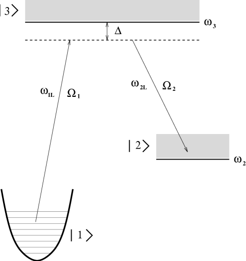
FIG. 1.: Schematic diagram of energy levels and couplings involved in the stimulated Raman process. $\Delta$ is the detuning, $\omega_{i}$, $\Omega_{iL}$, $i=1,2$ are the frequencies and the Rabi frequencies of the two lasers.

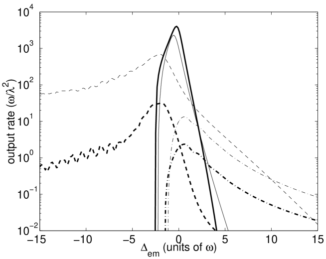
FIG. 2.: The rate of output as a function of $\Delta_{em}$ for atoms emerging from various different processes at temperatures $T=10\hbar\omega/k$ (bold line) and $T=150\hbar\omega/k$ (thin line). Solid line: $dn^{0}_{f}/dt$, output from the condensate component; Dashed line: $\sum_{j}dn^{j+}_{f}/dt$, from stimulated quantum evaporation; Dash-dotted line: $\sum_{j}dn^{j-}_{f}/dt$, from pair-breaking. A constant density of states $\rho(\omega_{{\bf k}})=1$ was used.

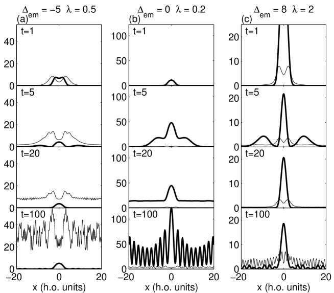
FIG. 3.: A one-dimensional demonstration of the temporal evolution of the coherent component (bold line) and the thermal component (thin line) of the output atomic density at $T=150\hbar\omega/k$ ($\sim 0.5T_{c}$) for different coupling strengths and detunings. (a) $\Delta_{em}=-5\omega$, $\lambda=0.5\omega$, (b) $\Delta_{em}=0$, $\lambda=0.2\omega$, and (c) $\Delta_{em}=8\omega$, $\lambda=2\omega$. The output density from the condensate has a steady component that remains near the trap; this part corresponds to the appearance of the bound states discussed after Eq. (69).

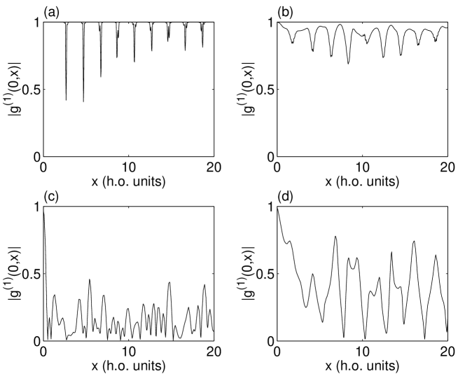
FIG. 4.: The first order coherence $g_{f}^{(1)}(x_{1},x_{2},t)$ of the output atoms as a function of $x=x_{2}$ for a fixed value of $x_{1}=0$ at time $t=100/\omega$, for (a) $T=10\hbar\omega/k,\Delta_{em}=0$ (Dominant coherent output), (b) $T=150\hbar\omega/k$, $\Delta_{em}=0$, (c) $T=150\hbar\omega/k,\Delta_{em}=-5\omega$ (dominant thermal output) and (d) $T=150\hbar\omega/k,\Delta_{em}=8\omega$ (dominant pair-breaking).

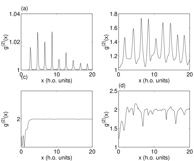
FIG. 5.: Equal-time single-point second order coherence function $g_{f}^{(2)}(x)$ of the output atoms at time $t=100/\omega$. Figures (a)-(d) correspond to the same cases plotted in figure 4 of the first-order coherence.

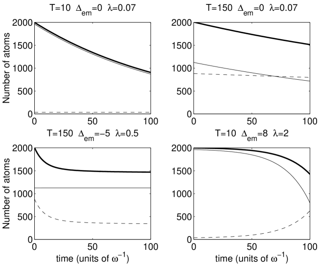
FIG. 6.: Evolution of the condensate (solid thin line) and excited (dashed line) atomic populations in the trap for few temperatures and coupling parameters. The bold solid line shows the total number of atoms in the trap as a function of time. In (a) ($T=10\hbar\omega/k$) and (b) ($T=150\hbar\omega/k$) the output is dominantly from the condensate. In (c) ($\Delta_{em}=-5\omega$) stimulated quantum evaporation from the higher excited levels is dominant and the remaining population in the trap is mainly the condensate and the lower excited levels. In (d) ($\Delta_{em}=8\omega$) the population of the lower excited levels increases due to pair-breaking, while the condensate depopulates.

in

REFERENCES

- [1] M.-O. Mewes, M. R. Andrews, D. M. Kurn, D. S. Durfee, C. G. Townsend, and W. Ketterle Phys. Rev. Lett. 78, 582 (1997)
- [2] M. R. Andrews, C. G. Townsend, H.-J. Miesner, D. S. Durfee, D. M. Kurn, and W. Ketterle Science 275, 637 (1997)
- [3] J. L. Martin, C. R. McKenzie, N. R. Thomas, J. C. Sharpe, D. M. Warrington, P. J. Manson, W. J. Sandle, and A. C. Wilson, J. Phys. B 32, 3065 (1999).
- [4] E. W. Hagley, L. Deng, M. Kozuma, J. Wen, K. Helmerson, S. L. Rolston and W. D. Phillips Science 283, 1706 (1999)
- [5] I. Bloch, T. W. Hänsch and T. Esslinger Phys. Rev. Lett. 82, 3008 (1999)
- [6] J. J. Hope Phys. Rev. A 55, 2531 (1997)
- [7] G. M. Moy and C. M. Savage Phys. Rev. A 56, R1087 (1997)
- [8] J. Jeffers, P. Horak, S. M. Barnett, and P. M. Radmore (Unpublished)
- [9] R. J. Ballagh, K. Burnett, and T. F. Scott Phys. Rev. Lett. 78, 1607 (1997)
- [10] H. Steck, M. Naraschewski, and H. Wallis Phys. Rev. Lett. 80, 1 (1998)
- [11] B. Jackson, J. F. McCann, and C. S. Adams, J. Phys. B 31, 4489 (1998).
- [12] M. W. Jack, M. Naraschewski, M. J. Collett, and D. F. Walls Phys. Rev. A 59, 2692 (1999)
- [13] Y.B. Band, M. Trippenbach and P.S. Julienne, Phys. Rev. A 59, 3823 (1999).
- [14] M. Edwards, D. A. Griggs, P. L. Holman, C. W. Clark, S. L. Rolston, and W. D. Philips, J. Phys. B 32, 2935 (1999).
- [15] Y. Japha, S. Choi, K. Burnett and Y. Band, Phys. Rev. Lett. 82 1079 (1999)
- [16] F. Dalfovo et. al., Phys. Rev. Lett. 75, 2510 (1995); J. Low. Temp. Phys. 104, 367 (1996); A. F. G. Wyatt, Nature 391, 56 (1998); A. Griffin, Nature 391, 25 (1998)
- [17] Z. Idziaszek, K. Rzazewski and M. Wilkens, J. Phys. B 32, L205 (1999).
- [18] A. Griffin Phys. Rev. B 53, 9341 (1996)
- [19] There are recent theories which go beyond HFB from considerations of microscopic interaction between particles eg. N. P. Proukakis, K. Burnett, and H. T. C. Stoof, Phys. Rev. A 57, 1230 (1998); N. P . Proukakis, S. A. Morgan, S. Choi and K. Burnett, Phys. Rev. A 58, 2435 (1998). These mainly result in small shifts in energies of excitations. We assume these differences are not as crucial in modelling an output coupler.
- [20] C. W. Gardiner, Phys. Rev. A 56, 1414 (1997); M. D. Girardeau, Phys. Rev. A 58, 775 (1998).
- [21] S. A. Morgan, S. Choi, K. Burnett and M. Edwards, Phys. Rev. A 57 3818 (1999)
- [22] C. Cohen-Tannoudji, J. Dupont-Roc, and G. Grynberg, Atom-photon interactions : basic processes and applications (Wiley, New-York, 1992). Complement .
- [23] R. J. Glauber, Phys. Rev. 130, 2529 (1963)
- [24] E. V. Goldstein and P. Meystre, Phys. Rev. Lett. 80 , 5036 (1998); E. V. Goldstein, O. Zobay, and P. Meystre, Phys. Rev. A 58, 2373 (1998).
- [25] M. Naraschewski and R. J. Glauber, Phys. Rev. A 59, 4595 (1999).
- [26] J. Javanainen, J. Ruostekoski, B. Vestergaard and M. R. Francis, Phys. Rev. A 59, 649 (1999).
- [27] R. J. Dodd, K. Burnett, M. Edwards, and C. W,. Clark Optics Express 1, 284 (1997)
- [28] Y. Castin and R. Dum, Phys. Rev. Lett. 77, 5315 (1996); 79, 3553 (1997);
- [29] Y. Castin and R. Dum, Phys. Rev. A 57, 3008 (1998)
- [30] D. S. Jin, M. R. Matthews, J. R. Ensher, C. E. Wieman, and E. A. Cornell, Phys. Rev. Lett. 78, 764 (1997).
- [31] S. Giorgini, Phys. Rev. A 57, 2949 (1998); P. O. Fedichev, G. V. Shlyapnikov and J. T. M. Walraven, Phys. Rev. Lett. 80, 2269 (1998); L. P. Pitaevskii and S. Stringari, Phys. Lett. A 235, 398 (1997); V. Liu, Phys. Rev. Lett. 79, 4056 (1997).
- [32] Y. Japha, and Y. B. Band (Unpublished)
- [33] E. A. Burt, R. W. Ghrist, C. J. Myatt, M. J. Holland, E. A. Cornell, C. E. Wieman, Phys. Rev. Lett 79, 337 (1997)
in