Multifractal analysis of normal RR heart-interbeat signals in power spectra ranges.

Abstract

Power spectral density is an accepted measure of heart rate variability. Two estimators of multifractal properties: Wavelet Transform Modulus Maxima and Multifractal Detrended Fluctuation Analysis are used to investigate multifractal properties for the three strongly physiologically grounded components of power spectra: low frequency (LF), very low frequency (VLF) and ultra low frequency (ULV). Circadian rhythm changes are examined by discrimination of daily activity from nocturnal rest. Investigations consider normal sinus rhythms of healthy 39 subjects which are grouped in two sets: 5-hour wake series and 5-hour sleep series. Qualitative arguments are provided to conjecture the presence of stochastic persistence in LF range, loss of heart rate variability during night in VLF range and its increase in ULF.

I Introduction

Power spectral analysis of normal RR- series of heart rate has gained popularity as a simple, non-invasive measurement capable of assessing dynamic changes in the autonomic nervous system’s control of heart rate Guide . Power spectrum means frequency analysis to identify superimposed oscillations which contribute to variations in heart rate. It has been observed fractal that in the very low frequency range, from 0.0003 to 0.04 Hz, the power spectral density decays as $1/f^{\beta}$. This property provides evidence of long range dependences in the data which, when viewed within the right range of scales, leads to the notion of fractality or self-similarity: statistical properties measured at some time scale look just like an appropriately scaled same statistical properties measured over a different time scale.

However long range dependences leave the small-time scale behavior (high frequency and low frequency components of the spectrum) essentially unspecified. In order to be capable of accounting for small time scales we need methods which deal with regularity, it is with differentiability, of stochastic processes. Traditionally to quantify and qualify local irregularities the spectrum of Hölder exponents, called multifractal spectrum is indicated Riedi ; FracMath . The practical estimations of exponents is performed in three steps. First, from the observed time series $X(t)$ one computes multiresolution coefficients $T_{X}(a,t)$, quantities that depent jointly on time $t$ and an analysis scale $a$. Second, one constructs the partition function $P(q,a)$ from these coefficients weighed by q powers. Third, one measures the slope $\tau(q)$ in $\log a$ of versus $\log P(q,a)$ diagram. The multifractality of $X(t)$ means that $\tau(q)\neq qH$.

The aims of the following are:

— To provide links between properties learned from multifractal studies and characterization of the heart control system obtained by power spectral density analysis in physiologically grounded frequency intervals. Especially, daily activity will be compared to nocturnal rest. By separating wake from sleep human stages we want to minimize effects related to nonstationarity in a signal. So far the problem whether the multifractal properties depend on a man activity is discussed and contradicting conjectures are suggested DayNight ; Kiyono2005 .

— To present in a compact and uniform way the numerical techniques used in discovering multifactal properties. We discuss results arisen from two most popular methods: Wavelet Transform Modulus Maxima BacryMuzyArnedo and Multifractal Detrended Fluctuation Analysis MDFA . Moreover, following Lashermes , we consider the linearization effect in scaling of a structure function $\tau(q)$ by searching for points where a multifractal spectrum concentrates.

The estimates are applied to two types of series: to a normal RR-signal extracted from ECG recordings and to the series obtained by integration of a normal RR-signal. The multifractal properties are statistical features. They are obtained numerically following heuristic procedures. So that results could depend on details of both - properties of series and numerical procedures. Therefore, for reliability of the discussed multifractality it should be important to confirm results in various ways Oswiecimka .

The paper is organized as follows. In Sec.II we give a brief physiological background to reasons of heart rate variability. In Sec.III the multifractal formalism is introduced and discussed. Then, Sec. IV, we shortly describe data which is used in our investigations. Sections V and VI contain the results: the group partition functions together with variety of linear fits which can be found to these functions (Sec. V) and the multifractal spectra estimated in physiologically grounded time intervals. The last section, Sec. VII, presents suggestions for further work. We believe that our considerations, though concentrated mostly on the purely descriptive aspect of multiscaling, are important in putting forward the research aimed on reasons for complex dynamics that is observed by the heart rate.

II Heart rate variability by power spectrum analysis

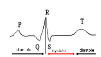
Figure 1: ECG diagram for a single heart period. Subsequent elements corresponds to atrial depolarization: P-wave, ventricular depolarization: QRS-complex and ventricular repolarization: T-wave.

The timing of a normal heart beat consists of three elements easily recognizable in an electrocardiogram (ECG), see Fig. 1. In a normal heart beat the following sequence of events must occur: P-wave (describing depolarization of atria), QRS-complex (associated to contraction of ventricles) and then T-wave (showing relaxation of ventricles after the contraction). The so-called normal sinus rhythm means that each P-wave is followed by QRS-complex and the rate is characterized by 60 to 100 beats per minute with 10% variation Guide . The time intervals between successive R-peaks of QRS-complex are called RR-series. Heart rate variability refers to increases and decreases over time in the RR interval. In Fig. 2 a RR-series is compared to the same data but shuffled at random. An-eye inspection hints that there must be a relation between consecutive heart beats.

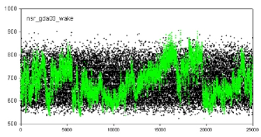
Figure 2: A series of RR normal heart beat intervals (green) and the same data shuffled at random. The series is 5-hour record of daily activity of a healthy subject(nsr_gda03_wake amgdata )

A heart beat is generated by the autonomous pacemaker, called sino-atrial node, located at the top of the right atrium. However, the frequency is mediated by the neural (autonomic nervous system — ANS) and hormonal (rennin - angiotensin - aldosterone system) activity Guide ; Jackson . This activity is controlled by large number of different feedbacks acting simultaneously. For example, both the blood pressure as well as changes in the blood pressure stimulates baroreceptors Malik , and baroreceptors generate a signal to ANS.

ANS consists of two parts which act antagonistically — the sympathetic subsystem activity accelerates the heart rate and enhances the heart muscle contractility while the parasympathetic subsystem activity elongates the interbeat intervals. This permanent conflict is supposed to be the reason for complex fluctuations which the normal heart rate displays. It is a widely accepted conjecture Guide ; Malik ; Gregory ; Jackson ; Sandercock ; Frenneaux ; Jong , strongly supported by physicists Ivanov ; filter ; Kotani ; Kiyono2005 ; Makowiec ; Physica04 that variability of the heart rate reveals the delicate balance between the two branches of ANS and even more — $1/f$ scaling in healthy heart rate requires the existence of this balance Struzik .

A recent introductory to the methodology of the heart rate variability can be found in Jong and discussion of autonomic system influence in Frenneaux . Here we concentrate on the so-called frequency-domain measures resulted from analysis of power spectral density of a RR tachogram Guide . To avoid nonstationarities short-time recordings (several minutes) are used. Three main spectral components are distinguished in this spectrum: very low frequency: $0.003<f<0.04$ Hz (VLF), low frequency $0.04<f<0.15$ Hz (LF) and high frequency: $0.15<f<0.4$ Hz (HF) components. Longer recording (hours) spectral analysis provides an additional range $f<0.003$ Hz termed ultra low frequency component (ULF).

The physiological explanation of ULF and VLF is less defined than other components. The power spectral density for these components is of power-low form $1/f^{\beta}$. The value of $\beta$ can discriminate healthy heart rate from a rate with heart failure fractal . Moreover, reduced levels of the spectral power have been identified as predictions of all-cause mortality (see Sandercock for discussion). There is some evidence that it is influenced by thermoregulatory mechanisms and humoral rennin-angiotensin system, but physical activity also notably influences to the power Roach .

The higher frequencies — HF component, are modulated predominantly by parasympathetic activity. A sino-atrial node responds to this activity at the respiratory frequency. LF component is modulated by both sympathetic and parasympathetic neural influence. The ratio of the spectral power LF to HF is used as a measure of sympathovagal balance. However this measure is found to be controversial Jong .

It is known that multifractal analysis can serve indicators of a state of ANS. The definite reduction of multifractal properties, namely the transition from multifractal to monofractal, is observed in multifractal picture of ECG of patients with congestive heart failure Ivanov ; filter . The modifications in multifractal spectra are observed in case of other heart diseases Kotani ; Makowiec ; MeyerStiedl . Following those investigations some heart rate variability measures have been proposed, e.g , spectrum width, spectrum location, curvature of a spectrum. Especially, it has been observed that a multifractal spectrum is distinct from a monofractal plot by existence of points (more than one) at which the spectrum is concentrated Makowiec . Speculations are continued that multifractal analysis offers potentially promising tools for heart rate variability assessments, but standards are lacking.

III Multifractal approach

Multifractal analysis of time series is strongly mathematically grounded, see for example FracMath ; Riedi . Roughly speaking by multifractal study one wants to express relations between points $X(t^{\prime})$ and a given point $X(t)$, where $t^{\prime}\in{\cal N}(t)$ belongs to some neighborhood of $t$, by comparing a part of series to a polynomial with a singularity exponent $h(t)$:

$$|X(t^{\prime})-X(t)|\sim K|t^{\prime}-t|^{h(t)}\qquad{\rm for}\quad t^{\prime}\in{\cal N}(t)$$ (1)

The singularity exponent $h$ is often called Hölder exponent. Typically a process $X(t)$ will posses many different singularities when moving $t$. The multifractal spectrum measures the frequency of occurrence of a given singularity exponent. Since singularity values change along the series vividly then the probability of occurrence is measured by the Hausdorff dimension of the subset of time where the same singularity exponent value is accounted:

$$D(h)=\dim_{H}\{t:h(t)=h\}$$ (2)

However transferring these ideas to numerical estimates of a series which arises from some natural phenomena is not obvious. Both tasks: extracting singularity exponents and evaluating the Hausdorff dimension, are numerically difficult and calculations cannot be performed automatically.

When one deals with discrete time series then special difficulty relates with determination of the neighborhood ${\cal N}(t)$ . In case of continuous data $x(t)$, the fractal singularity is estimated with respects to the small enough $|t-t^{\prime}|$ interval. But how to transfer this condition to a discrete signal? At the smallest possible interval, namely a unit interval, each two points can be connected by any function. If a regular function is chosen then the fractal dimension will be zero. Does it mean that the described procedure is useless? In Fig.3 we present a piece of series consisting of a hundred points which are divided into two equal size boxes. The question is whether the neighborhood consisting of 50 points or more can be considered as small enough to provide estimates for roughness of a series. In our opinion any scale is appropriate to discuss the fractal properties of a discrete time series. Following this belief we will continue to call our search as calculations of multifractal properties.

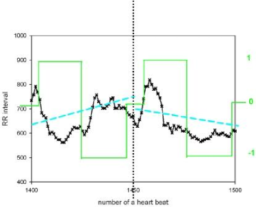
Figure 3: WTMM vs MDFA methods in a simplest form. A signal is divided into boxes of size 50 heart beats. In each box, the oscillations of a signal are represented by two estimates: a wavelet coefficient (here, the Haar wavelet is plotted by a solid line) and a fluctuation from a main trend (a dashed line plots the linear trend for a given box).

Both estimates: singularity exponent $h$ and its fractal dimension $D(h)$ can be found thanks to scaling properties of the partition function and their relation to a global characterization of a fractal object FracMath ; ArnedoBacryMuzy .

Basically, there are two approaches to construct the multiresolution coefficients:
(1) aggregation of a signal within a $K$-th box of a given size $n$, i.e., $X(n,K)={1\over n}\sum_{i=1}^{n}X(Kn+i)$,
and
(2) increment of a signal within a $K$-th box of a given size $n$, i.e., $X(n,k)=X(Kn+n)-X(Kn)$.

By the wavelet technique and detrended fluctuation method one deals with both: increments between carefully chosen averages are estimated. Having a signal divided into boxes of a given scale, see Fig. 3, the wavelet transformation in a $K$-th box: $T_{\psi}(n,K)$ measures the signal local oscillations inside a box. One can also estimate signal oscillations by measuring departures $F_{P_{m}^{K}}(n,K)$ of the signal from a polynomial trend $P_{m}^{K}$ of order $m$ found for points of $K$-th box. Finally, the partition function for a given scale is defined as the sum of either selected — local absolute value maxima in case of wavelets, or all — in case of detrended fluctuations, oscillations weighted by $q$ exponent. Both methods are heuristic and therefore below we give the precise mathematical formulas of estimates.

Let us assume that a series $\{X(i)\}$ is divided into boxes consisting of $n$ points. Then the following calculations lead to the partition functions $Z(n,q)$ and $F(n,q)$, respectively.

— In Wavelet Transform Modulus Maxima (WTMM) method a multiresolution coefficient is obtained as follows, BacryMuzyArnedo :

$$T_{\psi}(n,K)=\sum_{i\in K}X(i)\psi_{K}(n,i)$$ (3)

where $\psi_{K}(n,i)$ is the mother wavelet transformed to scale $n$ and shifted to $K$th box. Then the partition function $Z(n,q)$ is:

$$Z(n,q)=\sum_{K:\sup{local\ maxima\atop across\ finer\ scales}}|T_{\psi}(n,K)|^{q}$$ (4)

where sum takes supremum over so-called maxima lines, i.e., lines which link the local maxima at the present scale with the maxima at the previous scales.

— In Multifractal Detrended Fluctuation Analysis(MDFA) approach a multiresolution coefficient is defined as, MDFA :

$$S_{P_{m}^{K}}(n,K)=\left(\sum_{i\in K}[X(i)-{P_{m}^{K}}(i)]^{2}\right)^{\frac{1}{2}}$$ (5)

and then the partition function $S(n,q)$ is given as

$$F(n,q)=\sum_{K}S_{P_{m}^{K}}(n,K)^{q}$$ (6)

Let us notice that the supremum over the maxima lines, calculated in WTMM approach (4), provides the inter scale links while MDFA method works on each scale independently.

Dependence on $n$ of any partition function $P$ leads to so-called structure function $\tau(q)$ as follows:

$$P(n,q)\sim n^{\tau(q)}$$ (7)

and then by applying a Legendre transform to a curve $(q,\tau(q))$ one obtains the multifractal spectrum $(h,D(h))$:

$$h=\frac{d\tau(q)}{dq}\qquad D(h)=qh-\tau(q)$$ (8)

which links the singularity exponent value $h$ with its probability to appear $D(h)$ in a signal.

In case of a monofractal signal one expects a linear structure function $\tau(q)$ and then a corresponding spectrum should consists of one point $(h,D(h))$. But the numerics overestimate the real Hölder exponent $h$. Therefore the numerical results are sometimes called the coarse Hölder exponents Riedi . Additionally, the Legendre transform (8) significantly magnifies any small departures from linearity. Finally, what we obtain from numerical estimates are spectra which are far from being a point-like Makowiec ; Oswiecimka . However the maximum of a spectrum curve is directly related to the theoretical spectrum point and the maximum point is the highest occupied point of the whole spectrum Makowiec . A multifractal spectrum is distinct from a monofractal plot by existence of many highly occupied points. This feature is called the linearization effect and is suggested to be related with the nature of the process Lashermes .

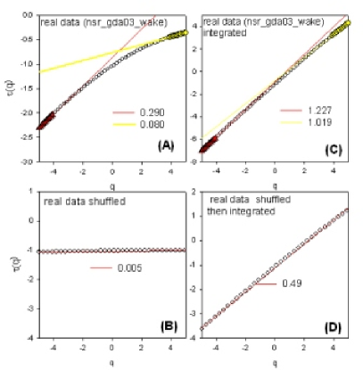
Figure 4: Structure functions $\tau(q)$ obtained by MDFA for a RR signal. (A) $\tau(q)$ for nsr_gda03_wake. (B) $\tau(q)$ for nsr_gda03_wake shuffled at random. (C) $\tau(q)$ for nsr_gda03_wake integrated.(D) $\tau(q)$ for nsr_gda03_wake shuffled at random and integrated. All linear fits provides $r^{2}$-errors greater than 0.98

In general when studying empirical data what we know is that negative moments, i.e., when $q<0$, are responsible for enhancing small fluctuations while positive moments, $q>0$, amplify large fluctuations. The right wing of a spectrum corresponds to negative moments and the left wing reflects properties collected for positive moments.

In Fig.4A we present the structure function found due to MDFA method to a series shown in Fig.2. The structure function $\tau(q)$ of the pure signal is concave and any linear fit is loaded by a large $r^{2}$-error. However, one can easily see that for $|q|>4$ line fits are justified (the linearization effect) what will result in emergence of two dense occupied points on $(h,D(h))$ plane: at $h=0.290$ and at $h=0.005$. The signal is multifractal. If the data is shuffled at random, then the corresponding partition function becomes a flat line, see Fig. 4B. The same result is obtained for a white noise — a canonical example of a monofractal signal. Its multifractal spectrum consists of a point $(0,1)$.

In the original detrended fluctuation analysis one deals with so-called profiles, see DFA . The profile can be thought as a signal obtained after integrating series. Dealing with series of integrated RR intervals one introduces a kind of smoothing since only growth in a data set is possible. Moreover, integrated series allows to study strength of independency in a series. In Fig. 4C the structure function obtained for the integrated series of nsr_gda03_wake is shown. Again the linear fits are provided for $|q|>4$. The linear approximations in these intervals give: 1.227 and 1.019 what locates the multifractal spectrum between these two points. Hence, the spectrum is moved right by about of 1 from the spectrum obtained from the pure series on the $(h,D(h))$ plane. However, if the data is independent then, see the structure function of integrated shuffled data in Fig. 4D, the linear fit provides the slope of $0.49$ what means that the spectrum is moved right but only by 1/2.

IV Heart interbeat interval data

The series called nsr_gda were collected from 39 healthy individuals (4 women, 35 men, the average age is $54\pm 7$) without past history of cardiovascular disease, with both echocardiogram and electrocardiogram in normal range. The left ventricle ejection fraction was normal (mean LVEF $=68.0\pm 4.7\%$). For each person the 24-hour ECG Holter monitoring was performed. The signal was digitized using Delmar Avionics recorder (Digitorder) and then analyzed and annotated using Delmar Accuplus 363 system (fully interactive method) by an experienced physician. The minimum number of qualified normal sinus beats required for the signal to enter the study is $85\%$. Moreover, the standard filters filter have been applied to smooth out the data.

From each signal the two 5-hour continuous subsets were extracted: diurnal and nocturnal. By extracting such subseries we wanted eliminate at least some sources of nonstationarities. The subsets were extracted manually, with regards to two easily recognizable stages: daily activity and sleep state. In most cases these periods are consistent with hours 15:00–20:00 for the daily activity and 0:00–5:00 for the sleep state. In the following we will denote the subseries as nsr_gda_wake, nsr_gda_sleep, respectively. All RR-series and their subseries are accessible on request amgdata .

Since the WTMM method requires data sets longer than $2^{14}$, then some of the sleep subseries have to be excluded from WTMM calculations. So that nsr_gda_sleep group consists of 34 data sets in case of WTMM calculations.

V Scaling properties of partition functions

Both partition functions $Z(n,q)$ and $F(n,q)$ are calculated by tools accessible from PhysioNet physionet . Namely, we work with two Physionet packages: multifractal.c (prepared by Y. Ashkenazy) and dfa.c (prepared by J.Mietus, C-K Peng, and G. Moody ) adapted by us and accessible from amgdata

For each individual series, regarded as either directly as a sequence of RR intervals, or as a sequence of integrated RR intervals, the partition function was found for all $q$ in $[-5,5]$ with a step $0.1$, for scales from $n=10$ to almost $1000$ heart beats. In all calculations we applied the third derivative of a Gaussian as a mother wavelet in WTMM method, (thus up to quadratic polynomial dependencies in $t$ are eliminated by WTMM) and a quadratic polynomial as a detrending fit (MDFA). Such setting of parameters has been found by us as less dependent on the length of test series — localization of spectra is stable (WTMM) and width of spectra is stable (MDFA).

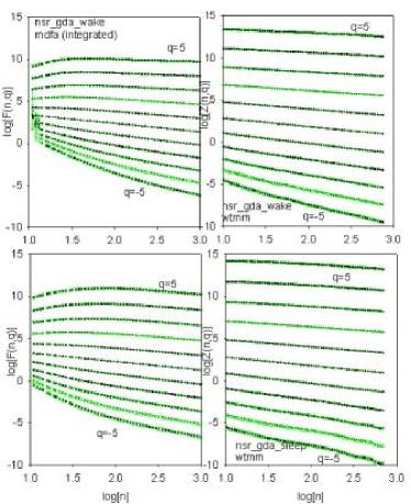
Figure 5: Group average of partition functions calculated by MDFA and WTMM methods for each element of the group and for different $q=-5,-4,\dots,4,5$. In green, statistical errors of estimates (standard deviation of a group $\backslash\sqrt{N}$, where $N$ number of elements in the group) are given.

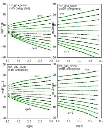
Figure 6: Group average of partition functions calculated by MDFA and WTMM methods for each integrated signal of the group for different $q=-5,-4,\dots,4,5$. In green, statistical errors of estimates (standard deviation of a group $\backslash\sqrt{N}$, where $N$ number of elements in the group) are given.

The partition functions $Z(n,q)$ and $F(n,q)$, shown in Figs 5, 6, are group averages obtained from the partition functions found for each individual series by WTMM and MDFA methods, respectively. We present $Z(n,q)$ and $F(n,q)$ for $q$-representatives $\{-5,-4,\dots,4,5\}$ together with their statistical errors. We found errors satisfactory low (with significance level $p<0.05$ ) to discriminate values of particular $q$s. Therefore we could turn to searching for power-law scalings of these functions. To reliably infer power-law scaling, a straight line in log-log plot has to be established. In Figs 5, 6 the log-log scale is used to enhance visually linear relations between log[scale] and log [partition function].

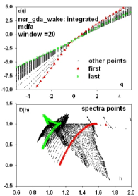
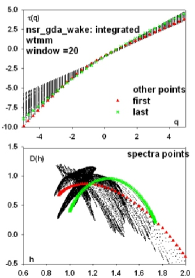
Figure 7: The structure functions and spectra obtained when the linear fits are found for subsequent 20 points of the corresponding partition functions. Group averages for integrated nsr_gda_wake obtained by both methods for pure series (upper panel) and integrated series (bottom panel).

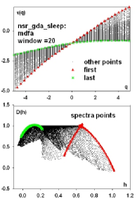
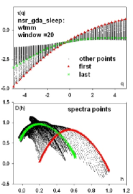
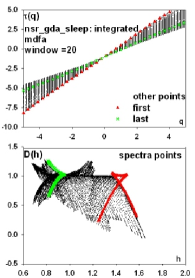
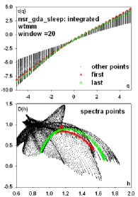
Figure 8: The structure functions and spectra obtained when the linear fits are found for subsequent 20 points of the corresponding partition functions. Group averages for integrated nsr_gda_wake obtained by both methods for pure series (upper panel) and integrated series (bottom panel).

It appears that the partition functions $F(n,q)$ change their dependence on a scale. Especially, the change is noticeable in case of pure series. Since numerical calculations are sensitive to details of curves, we evaluate subsequently local slopes of all functions: $\log F(n,q)$ vs $\log n$ as well as $\log Z(n,q)$ vs $\log n$ to observe changes in scalings. In particular, we calculate linear fits for subsequent 20 points of each partition function and move with the starting point from 20th heart beat to the end of series. This way we obtain the variety of possible approximations and then we can ask how one can estimate fine scale or/and large scale limits properties.

The results – local structure functions and resulting local spectra plots are shown in Figs 7, 8. The first structure function $\tau_{first}(q)$, labeled first (red plots) starts at the 20th heart beat. The plots labeled last in the figures correspond to $\tau_{last}(q)$ obtained in the last possible but smaller than 1000th heart beat (green plots). One has to be aware that 20 points at fine scales correspond to about several heart beats while 20 points at large scales cover few hundred heart beats since a scale box grows geometrically with a ratio $2^{0.05}$. The spectra are plotted below the corresponding structure functions. One can see that the ’body’ of each spectrum occupies a wide part of a plane $(h,D(h))$. The strange structures appearing in some of spectra are consequences of Legendre transformation (8) when treated by numerical methods.

Both methods MDFA and WTMM provide similar results in case of pure series. The fine scales are significantly separated from large scales: the first-plots are centered at $h=0.6$ while last-plots are concentrated around $h=0.2$. The maxima of corresponding spectra are located similarly on $(h,D(h))$ -plane and widths of corresponding spectra are in similar relations: the fine scale widths are significantly greater than the large scale spectra. These results might suggest presence of plenty independent stochastic noises actively influencing dynamic properties of heart rate in short time scales.

The integrated series are expected to provide spectra moved right by 1 from the pure series. It appears that this simple relation is about to be satisfied only in case of the spectra of wake series treated by MDFA method. In case of the sleep data we see that the spectrum corresponding to large scales is located in $h<1$ area. This observation suggests that nocturnal series are characterized by stronger independence between subsequent heart beats than diurnal series. In case of WTMM method both limits: fine and large scale provide spectra centered similarly at about $h=1.2$. Therefore one can conjecture that WTMM spectra of integrated series represent some average multifractal characteristics.

VI Spectra

In the following we search for the best linear fits of partition functions in the particular time intervals. These intervals, transfered into number of beats, are directly related to the physiology of the heart rate control and the classical spectral analysis as it was described in Sec II. The group structure functions and the group spectrum plots are presented as follows, see Fig.9:

• 10–25 heart beats that cover times from 8 to 20 seconds, what allows us to estimate early compensatory mechanism represented by LF.

• 25–300 heart beats that last from 20 seconds to 4 minutes, what examines the activity of rennin-angiotensin-aldosterone system and other neurohormones, which additionally activates the sympathetic nervous system and corresponds to VLF.

• over 300 heart beats, i.e., times over 4 minutes allow to study frequencies smaller than 0.003Hz, hence we are within ULF component.

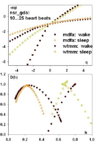
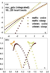
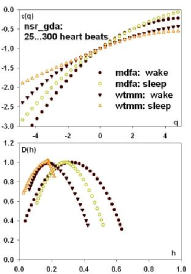
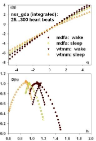
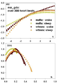
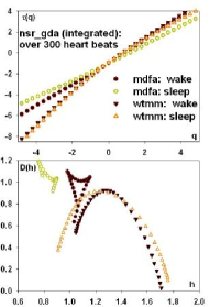
Figure 9: The structure functions and spectra obtained when the linear fits are for heart beat intervals physiologically motivated. The intervals are described in plot titles. Every third points are plotted to emphasize centers of spectral point concentration.

We can not enter into the high frequency HF range because of numerical instabilities occurring when $q<0$.

It appears that in short times, less than 20 seconds, each method locates the multifractal spectra in different intervals of $h$. Both pure spectra: wake and sleep are in $h\in(0.5,1.0)$ in case of MDFA while maxima of WTMM spectra are about $h=0.2$ though there is a noticeable center of WTMM wake spectrum points at $h=0.6$. The spectra obtained from integrated series sustain this observations — WTMM plots are significantly separated from plots obtained by means of MDFA. It denotes that roughness of signals measured in scales smaller than 25 beats (a half of a box from Fig.3) is considerable differently estimated by both methods. Yet both methods indicates on presence of strong persistence in series, because the spectra contain singularity exponents with $h>0.5$. The persistence is usually related to burstiness or clustering in data — fluctuations larger or smaller than a given level happen subsequently, i.e., much often than in the case of independent observations.

Heart rate in LF range is strongly influenced by oscillations in blood pressure. Basically the baroreflex is the modulator of RR interval in a healthy subject. However there are receptors which control the other aspects of proper blood supply, and which activity can be evaluated by the level of randomness in LF range Sandercock . Both multifractal methods produce wide spectra what can be attributed to a large variety of controlling elements under which a cardiovascular system maintains blood supply during daily human activity. Moreover, the randomness point $h=0.5$ belongs to both spectra and it could provide an indicator of the level of the baroreflex sensitivity. MDFA plots of integrated series are moved toward a multifractal range which corresponds to a series of integrated random walk. Thus RR intervals are seen as rather independent of each other. However WTMM provides plots with maxima highly occupied at about $h=0.85$ for sleep series and around $h=0.95$ in case of wake series.

DFA picture of VLF range, Fig.9 plots of middle panel, again provides a huge variety of scaling exponents in case of daily activity $h\in(0,0.6)$ with two centers where spectrum points are densely located: at maximum $h=0.3$ and at $h=0.6$. WTMM spectrum in VLF range gives the wake spectrum narrower and mainly concentrated at its left wing, i.e., for $h<0.2$. Thus comparing the two methods one can say that WTMM enhances influence of large oscillations which are contained in $\tau(q)$ when $q>0$, while MDFA amplifies role of small fluctuations expressed by $\tau(q)$ with $q<0$. Both wake spectra are wider than the spectra of sleep series and the sleep spectra are located inside the corresponding wake spectra. Thus one can conjecture loosing variability in heart rate (measured by a pool of scaling exponents) during the night rest in VLF range.

The integrated wake and sleep spectra corresponding to VLF component exhibit noticeable separation from each other: the sleep spectra are moved to left, to lower Hölder exponents, namely, $h\in(0.6,1)$. Both sleep curves are characterized by densely occupied left wings. Hence the roughness of night series is significantly wilder. The main parts of the wake spectra occupy the similar range of $h$, i.e., $h\in(1,1.2)$. This means that WTMM wake spectrum is moved right by 1 when compared it to the pure series result but MDFA one not. However there is a spectrum center at $h=1.5$.

The third frequency component UHF corresponds to the time range where long range dependences are usually searched. Therefore it is not a surprise that our results recalls results obtained by others, see Ivanov ; filter ; Kotani ; Makowiec . In case of pure series all spectra are characterized by similar set of singularity exponents $h$ concentrated at $h=0.2$ and the widths of WTMM spectra are wider than the corresponding MDFA ones. Moreover, MDFA results received for integrated series reveal global properties known thanks to DFA studies DFA : the healthy heart long range correlations are characterized by $\alpha_{DFA}=1$ for a daily activity and by $\alpha_{DFA}=0.8$ during a nigh rest. WTMM spectra for integrated series differentiates day and night series by spectral width: the sleep spectrum is significantly wider than the wake one. However, the left wings of these spectra - consisting of many points, are located at the same $h$ as it is found by DFA.

VII Conclusions

Many naturally occurring empirical time series violate the assumption of independence of subsequent elements. Instead the data often point at the presence of strong temporal correlations. Relating these correlations with dynamic properties of a system under study is challenging.

Heart rate variability is a measure of fundamental aspects of a human physiology. It is known that frequency domain analysis of heart rate provides predictors of mortality in chronic heart failure — LF is a predictor for sudden cardiac death while VLF and ULV are predictors for all-causes mortality, see Guide ; Frenneaux ; Jong ; Sandercock .

In the following, basing on the descriptive rather aspect of multiscaling, we have analysed scaling properties of average multifractal partition functions in these physiologically grounded interbeat intervals: LF, VLF and ULF, following normal RR intervals of 39 healthy subjects. The data was grouped according to the circadian rhythm (wake and sleep series), the methods of multifractal analysis (WTMM and MDFA approach), and RR intervals were compared to integrated RR intervals. By applying different numerical methods we wanted to determine some objective properties hidden in series considered which discriminate daily heart activity from its nocturnal rest. In general, we observed loss of heart rate variability during night in VLF range and its increase in time corresponding to ULF component.

However, we have also found that details of multifractal properties such as spectrum width and location are different for different numerical methods. A partition function obtained by WTMM remembers about the strength of oscillations in a signal read in finer scales while MDFA provides at each scale an independent partition function. Therefore the relations between scales are more consistent with each other in case of WTMM spectra seen in different scales. It is specially noticeable in case of integrated series. The study of integrated RR-intervals has put a significant impact in evaluation of the participation of independent stochastic sources. We hope that all these differences would lead to additional tools allowing to quantify and qualify neural and humoral control of heart rate.

Acknowledgments This work was supported by the Rector of Gdansk University — project: BW$/$5400-5-0220-7

References

- (1) Heart Rate Variability. Standards of measurement, physiological interpretation, and clinical use. Eur.Heart J. 17, 354 (1996)
- (2) M.Kobayashi and T.Musha, 1/f fluctuation of heartbeat period.IEEE Trans.Biomed.Eng. BME-29 456–457 (1982); C. K. Peng, J. Mietus, J. Hausdorff, S. Havlin, H. E. Stanley, and A. L. Goldberger, Long-Range Anticorrelations and Non-Gaussian Behavior of the Heartbeat Phys.Rev.Lett. 70 1343 (1993); Y.Yamamoto and R.L.Hughson, On the fractal nature of heart rate variability in humans: effects of data length and beta-adrenergic blockade. Am.J.Physiol. 266 R40-R49(1994)
- (3) K.J. Falconer, Fractal Geometry - Mathematical Foundations and Applications John Wiley, Second Edition, 2003;
- (4) R.H. Riedi. Multifractal Processes. pp 625–716, in Long-range Dependence: Theory and Applications editors: P. Doukhan, G. Oppenheim and M. S. Taqqu, Cambridge Ma, Birkhäuser, 2001; W.Willinger, V.Paxson, R.H.Riedi, M.S.Taqqu pp1–38 in Long-range Dependence: Theory and Applications editors: P. Doukhan, G. Oppenheim and M. S. Taqqu, Cambridge Ma, Birkhäuser, 2001.
- (5) L.A.N. Amaral, P.Ch. Ivanov, N. Aoyagi, I. Hidaka, S. Tomono, A. L. Goldberger, H.E. Stanley and Y. Yamamoto, Behavioral- independent features of complex heartbeat dynamics. Phys. Rev. Lett. 86 6026–6029 (2001); L.A.N. Amaral, D.J.B. Soares, L.R.da Silva, L.S.Lucena, M.Saito, H.Kumano, N.Aoyagi and Y. Yamamoto, Power law temporal auto-correlations in day-long record in human physical activity and their alternation with disease. Eurphysics Lett. 66(3) 448-454 (2004)
- (6) K.Kiyono, Z.R.Struzik, N.Aoyagi, F.Toga and Y. Yammamoto. Phase Transition in a Healthy Human Heart Rate. Phys.Rev.Lett. 95 058101 (2005)
-
(7)
E. Bacry, J. F. Muzy and A. Arnedo. Singularity spectrum of fractals signals from wavelet analysis: Excact results. J. Stat. Phys. 70 635-374 (1993)
J.F. Muzy, E. Bacry and A. Arneodo. Multifractal formalism for fractal signals: The structure-function approach versus the wavelet-transform modulus-maxima method. Phys. Rev. E 47 875 (1993). - (8) J.W. Kantelhardt, S.A. Zschiegner, E. Koscielny-Bunde, S. Havlin, A. Bunde and H.E. Stanley. Multifractal detrended fluctuation analysis of nonstationary time series. Physica A 316 87 (2002).
- (9) B.Lashermes, P.Abry and P. Chainais. New insighths into the estimation of scaling exponents. Int.J.of Wavelets, Multiresolution and Information Processing 2 No 4 497–523 (2004)
- (10) P.Oświȩcimka, J.Kwapień, and S. Dro/.zd/.z, Wavelet versus detrended fluctuation analysis of multifractal structures. Phys.Rev.E 74 016103-1 (2006)
- (11) G.Jackson, C.R.Gibbs, M.K.Davies, and G.Y.H.Lip. ABC of heart failure. Pathophysiology. British Med.J. 320 167–170 (2000)
- (12) M. Malik, Heart Rate Variability and Baroreflex Sensitivity in Cardiac Electrophysiology in D. P. Zipes, J. Jalife (Eds.) From Cell To Bedside, 4th edition, Saunders, 2004
- (13) M.E. Gregory, R.J. Cody, E.Nuziata and P.F. Binkley. Early Left Dysfunction Elicits Activation of Sympathetic Drive and Attenuation of Parasympathetic Tone in in Paced Canine Model of Congestive Heart failure. Circulation 92 551 (1995)
- (14) M.P.Freneaux. Autonomic changes in patients with heart failure and in post-myocardial inf raction patients. Heart 90 1248-1255 (2004)
- (15) M.J.De Jong and D.C.Randall. Heart rate variability analysis in the assessment of autonomic function in heart failure. J.Cardiovasc. Nurs. 20 186–196 (2005).
- (16) G.R.H. Sandercock and D.A. Brodie, The Role of heart Variability in Prognosis for Different Modes of Death in Chronic Heart Failure. Pacing Clin. Electrophysiology 29(8), 892-904 (2006)
-
(17)
P.Ch. Ivanov, M.G. Rosenblum, C.-K. Peng, J. Mietus, , S. Havlin, H.E. Stanley and A.L. Goldberger, Scaling behaviour of heartbeat intervals obtained by wavelet-based time-series analysis. Nature 383 323 (1999);
P.Ch. Ivanov, L.A.N. Amaral, A.L. Goldberger, S. Havlin, M.G. Rosenblum, H.E. Stanley and Z.R. Struzik. From 1/f noise to multifractal cascades in heartbeat dynamics. Chaos 11 641 (2001) - (18) P.Ch. Ivanov, L.A.N. Amaral, A.L. Goldberger, S. Havlin, M.G. Rosenblum, Z.R. Struzik and H.E. Stanley. Multifractality in human heartbeat dynamics. Nature 399 461 (1999)
- (19) K.Kotani, Z.R.Struzik, K. Takamasu, H.E.Stanley and Y. Yamamoto. Model for complex heart rate dynamics in health and diseases Phys.Rev.E 72 041904 (2005)
- (20) D.Makowiec, R.Gała̧ska, A.Dudkowska, A.Rynkiewicz and M.Zwierz. Lon-range dependencies in heart rate signals - revisited. Physica A 369 632–644 (2006)
- (21) Y. Ashkenazy, S. Havlin, P. Ch.Ivanov, C.-K Peng, V. Schultte-Frohlinde and H. E. Stanley. Magnitude and sign scaling in power-law correlated time series. Physica A 323 19–41 (2003); P. Ch. Ivanov, Z. Chen, K.Hu and H. E. Stanley. Multiscale aspects of cardiac control. Physica A 344 685 (2004)
- (22) Z.R. Struzik J. Hayano, S. Sakata, S. Kwak, and Y. Yamamoto. 1/f Scaling in Heart rate Requires Antagonistic Autonomic Control. Phys.Rev.E 70 050901(R) (2004)
- (23) M. Meyer and O. Stiedl, Self-affine fractal variability of human heartbeat interval dynamics in health and disease. Eur. J. App. Physiol.90 305–316 (2003)
- (24) A. Arnedo, E. Bacry and J. F. Muzy. The Thermodynamics of fractals revisited with wavelets. Physica A 213 232 (1995)
- (25) C.-K. Peng, S.V. Buldyrev, S. Havlin, M.Simons, H.E. Stanley and A.L. Goldberger. Quantification of scaling exponents and crossover phenomena in nonstationary heartbeat time series. Phys.Rev.E 49 1685 (1995)
- (26) D.Roach, A.Sheldon, w.Wilson et al.Temporarally localized contributions to measures of large-scale heart rate vatriability Am.J.Physiol. 274 H1465-71 (1998)
- (27) A.L. Goldberger, L.A.N. Amaral, L. Glass, J.M. Hausdorff, P.Ch. Ivanov, R.G. Mark, J.E. Mietus, G.B. Moody, C.-K. Peng, H.E. Stanley. PhysioBank, PhysioToolkit, and PhysioNet: Components of a New Research Resource for Complex Physiologic Signals. Circulation 101(23):e215-e220 [Circulation Electronic Pages; ]; 2000 (June 13).
- (28) Series considered can be downloaded from http://iftia9.univ.gda.pl/d̃anka/DATA