Graph animals, subgraph sampling and motif search in large networks

Abstract

We generalize a sampling algorithm for lattice animals (connected clusters on a regular lattice) to a Monte Carlo algorithm for ‘graph animals’, i.e. connected subgraphs in arbitrary networks. As with the algorithm in [N. Kashtan et al., Bioinformatics 20, 1746 (2004)], it provides a weighted sample, but the computation of the weights is much faster (linear in the size of subgraphs, instead of super-exponential). This allows subgraphs with up to ten or more nodes to be sampled with very high statistics, from arbitrarily large networks. Using this together with a heuristic algorithm for rapidly classifying isomorphic graphs, we present results for two protein interaction networks obtained using the TAP high throughput method: one of Escherichia coli with 230 nodes and 695 links, and one for yeast (Saccharomyces cerevisiae) with roughly ten times more nodes and links. We find in both cases that most connected subgraphs are strong motifs ($Z$-scores $>10$) or anti-motifs ($Z$-scores $<-10$) when the null model is the ensemble of networks with fixed degree sequence. Strong differences appear between the two networks, with dominant motifs in E. coli being (nearly) bipartite graphs and having many pairs of nodes which connect to the same neighbors, while dominant motifs in yeast tend towards completeness or contain large cliques. We also explore a number of methods that do not rely on measurements of $Z$-scores or comparisons with null models. For instance, we discuss the influence of specific complexes like the 26S proteasome in yeast, where a small number of complexes dominate the $k$-cores with large $k$ and have a decisive effect on the strongest motifs with 6 to 8 nodes. We also present Zipf plots of counts versus rank. They show broad distributions that are not power laws, in contrast to the case when disconnected subgraphs are included.

I Introduction

Recently, there has been an increased interest in complex networks, partly triggered by the observation that naturally occurring networks tend to have fat-tailed or even power law degree distributions faloutsos ; barabasi . Thus real-world networks tend to be very different from the completely random Erdös-Renyi bollobas networks that have been much studied by mathematicians, and which give Poissonian degree distributions. In addition, most networks have further significant properties that arise either from functional constraints, from the way they have grown (fat tails, e.g., are naturally explained by preferential attachment), or for other reasons. As a consequence, a large number of statistical indicators have been proposed to distinguish between networks with different functionality (neural networks, protein transcription networks, social networks, chip layouts, etc.) and between networks which were specially designed or which have grown spontaneously (such as, e.g. the world wide web), under more or less strong evolutionary pressure. These observables include various centrality measures newman_SIAM , assortativity (the tendency of nodes with similar degree to link preferentially) newman_SIAM , clustering watts-stro ; newman_clust , different notions of modularity barabasi ; ravasz ; girvan ; ziv ; rosvall , properties of loop statistics stadler , the small world property (i.e., slow increase of the effective diameter of the network with the number of nodes) milgram , bipartivity (the prevalence of even-sized closed walks over closed walks with an odd number of steps) estrada , and others.

The frequency of specific subgraphs form a particular class of indicators. Subgraphs that occur more frequently than expected are referred to as motifs, while those occurring less frequently are anti-motifs milo ; shen-orr ; vasquez ; kashtan . Typically, motif search requires a null model for deciding when a subgraph is over- or under-abundant. The most popular null model so far has been the ensemble of all random graphs with the same degree sequence. This popularity is largely due to the fact that it can be simulated easily by means of the so-called ‘rewiring algorithm’ besag ; maslov . As we shall see, however, in the present analysis its value is severely limited, because it gives predictions that are too far from those actually observed. Other null models that retain more properties of the original network have been suggested milo ; mahadevan , but have received much less attention. Analytic approaches to null models are discussed in Refs. newman_park1 ; newman_park2 ; foster .

I.1 Motifs and the Search for Structure

Up to now, motif search has been mainly restricted to small motifs, typically with three or four nodes. Certain specific classes of larger subgraphs have been examined in Refs. class1 ; kashtan2004b ; vasquez . With the exception of Ref. baskerville , few systematic attempts have been made to learn about significant structures at larger scale, by counting all possible subgraphs (for a different approach to the discovery of structure than discussed here see the work on inference of hierarchy in Ref. clauset ).

One reason for this is that the number of non-isomorphic (i.e. structurally different) subgraphs in any but the most trivial networks increases extremely fast (super-exponentially) with their size. For instance, the number of different undirected graphs with 11 nodes is $\approx 10^{9}$ briggs . Thus exhaustive studies of all possible subgraphs with $>10$ nodes becomes virtually impossible with present-day computers. But just because of this inflationary growth, counts at intermediate sizes contain an enormous amount of potentially useful information. Another obstacle is the notorious graph isomorphism problem kobler ; faulon , which is in the NP class (though probably not NP complete toran ). Existing state of the art programs for determining whether any two graphs are isomorphic nauty remain too slow for our purpose. Instead, we shall use heuristics based on graph invariants similar to those put forward in Ref. baskerville , where intermediate size motifs and anti-motifs in the protein interaction network of Escherichia coli were detected.

The last problem when studying larger motifs, and the main one addressed in the present work, is the difficulty of estimating how often each possible subgraph appears in a large network, i.e. of obtaining a ‘subgraph census’. Most studies so far were based on exact enumeration. In a network with $N$ nodes, there are ${N\choose n}$ subgraphs of size $n$. With $N=500$ and $n=6$, say, this number is $\approx 5\times 10^{11}$. In addition, most of the subgraphs generated this way on a sparse network would be disconnected, while connected subgraphs are of more intrinsic interest. Thus some statistical sampling is needed. If one is willing to generate disconnected as well as connected subgraphs, then uniform sampling is simple: Just choose random $n$-tuples of nodes from the network baskerville . Uniform sampling connected subgraphs is less trivial. To our knowledge, the only work which addressed this systematically was Kashtan et al. kashtan2004b (for a less systematic approach, see also spirin ). There, a biased sampling algorithm was put forward. While generating the subgraphs is fast, computing the weight factor needed to correct for the bias is $\exp[O(n)]$, making their algorithm inefficient for $n\geq 7$.

I.2 Graph Animals

In the present paper we exploit the fact that sampling connected subgraphs of a finite graph resembles sampling connected clusters of sites on a regular lattice. The latter is called the lattice animal problem animals , whence we propose to call the subgraph counting problem that of graph animals. It is important to recognize obvious differences between the two cases. In particular, lattices are infinite and translationally invariant, while networks are finite and heterogeneous (disordered). For lattice animals one counts the number of configurations up to translations (i.e. per unit cell of the lattice), while on a network the quantity of immediate interest is the absolute number of occurrences of particular subgraphs. Still, apart from these issues, the basic operations involved in both cases coincide.

Algorithms for enumerating lattice animals exactly exist and have been pushed to high efficiency jensen , but are far from trivial redner . Due to disorder, we should expect the situation to be even worse for graph animals. Algorithms for stochastic sampling of lattice animals are divided into two groups: Markov chain Monte Carlo (MCMC) algorithms take a connected cluster and randomly deform it while preserving connectivity stauffer ; dickman ; pivot , while ‘sequential’ sampling algorithms grow the cluster from scratch leath ; hsu ; gfn1998 ; care . Even for regular lattices, MCMC algorithms seem less efficient than growth algorithms hsu . For networks, this difference should be even more pronounced, since MCMC algorithms would dwell in certain parts of the network, and averaging over the different parts costs additional time. Thus we shall in the following concentrate only on growth algorithms.

All growth algorithms similar to those in leath ; hsu ; gfn1998 ; care produce unbiased samples of percolation clusters. As explained in Sec. II, this means that they sample clusters or subgraphs with non-uniform probability (for an alternative algorithm, see Redner79 ). Consequently, computing graph animal statistics requires the computation of weights to be assigned to the clusters, in order to correct for the bias. In contrast to the algorithm in Ref. kashtan2004b , the correct weights are easily and rapidly calculated in our graph animal algorithm. This is its main advantage.

I.3 Summary

In Sec. II we present the graph animal algorithm in detail. The method used to handle graph isomorphism is briefly reviewed in Sec. III. Extensive tests, mostly with two protein interaction networks, one for E. coli with 230 nodes and 695 links ecoli , and one for yeast with 2559 nodes and 7031 links yeast , are presented in Sec. IV footnote . Both networks were obtained using the TAP high throughput method. In particular, our algorithm involves as a free parameter a percolation probability $p$. For optimal performance, in lattice animals $p$ should be near the critical value where cluster growth percolates hsu . We show how the performance for graph animals depends on $p$, on the subgraph size $n$, and on other parameters. In Sec. V we use our sampling method to study these two networks systematically. We verify that large subgraphs with high link density are overwhelmingly strong motifs, while nearly all large subgraphs with low link density are anti-motifs vasquez ; baskerville – although our data show much more structure than suggested by the scaling arguments of vasquez . We also find striking differences in the strongest motifs for the two networks. Dominant motifs for the E. coli network are either bipartite or close to it (with many nodes sharing the same neighbors) while ‘tadpoles’ with bodies consisting of (almost) complete graphs dominate for yeast. Our conclusions and discussions of open problems are given in Sec. VI.

The present work only addresses undirected networks, but the graph animal algorithm works without major changes also for directed networks. Due to the larger number of different directed subgraphs, an exhaustive study of even moderately large subgraphs is much more challenging newpaper .

II The Algorithm

In this section we explain how our algorithm achieves uniform sampling of connected subgraphs in undirected networks. The graph animal algorithm executes a generalization of the Leath algorithm for lattice animals. The observation central to the work in Refs. leath ; hsu ; care is that the animal and percolation ensembles concern exactly the same clusters. The only difference between the two ensembles is that clusters in the percolation ensemble have different weights, while all clusters with the same number of nodes (sites) have the same weight in the animal ensemble. We focus on site percolation stauffer-aharony . Bond percolation could also be used hsu , but this would be more complicated and is not discussed here.

II.1 Leath growth for graph animals

For regular lattices and undirected networks we use the following epidemic model for growing connected clusters of sites leath :
(1) Choose a number $p\in[0,1]$ and a maximal cluster size $n_{\rm max}$. Label all sites (nodes) as ‘unvisited’.
(2) Pick a random site (node) $i_{0}$ as a seed for the cluster, so that the cluster consists initially of only this site; mark it as ‘visited’.
(3) Do the following step recursively, until all boundary sites of the cluster have been visited, or until the cluster consists of $n_{\rm max}$ sites, whichever comes first: (Note that a boundary site of a cluster $C$ is a site which is not in $C$, but which is connected to $C$ by one or more edges).
(A) Choose one of the unvisited boundary sites of the present cluster, and mark it as visited; (B) With probability $p$ join it to the cluster.
Once a boundary site has been visited, it cannot later join the cluster; it either joins the cluster when it is first visited (with probability $p$) or is permanently forbidden to join (with probability $1-p$).

The order in which the boundary (or ‘growth’) sites are chosen influences the efficiency of the algorithm, but this is irrelevant for the present discussion. The growth algorithm can be seen as an idealization of an epidemic process (‘generalized’ or SIR epidemic mollison ; grass ) with three types of individuals (Susceptible, Infected, Removed). Starting with a single infected individual with all others susceptible, the infected individual can infect neighbours during a finite time span. Everyone either gets infected or doesn’t at his/her first contact. The latter are removed, as are the infected ones after their recovery, and do not participate in the further spread of the epidemic.

Assume that for some fixed node $i_{0}$, a connected labeled subgraph $G^{\ell}$ exists, which contains $i_{0}$ and has $n<n_{\rm max}$ nodes and $b$ visited boundary nodes. The chance that precisely this particular labeled subgraph will be chosen using the algorithm is

$$P_{G^{\ell}}(p;i_{0})\equiv P_{nb}(p;i_{0})=p^{n-1}(1-p)^{b}\;.$$ (1)

Since an independent decision is made at each boundary site, this is indeed the probability for $n-1$ sites to be selected to join the cluster, while $b$ sites are rejected.

Denote by $c(G^{\ell})$ the indicator function for the existence of $G^{\ell}$, i.e. $c(G^{\ell})=1$ if the subgraph exists in the network, and $c(G^{\ell})=0$ else. Furthermore, denote by $c(G^{\ell};i_{0})$ the explicit indicator that $G^{\ell}$ exists and contains the node $i_{0}$. Then the total number of occurrences of the unlabeled subgraph $G$ is given by

$$c_{G}=n^{-1}\sum_{i=1}^{N}c_{G,i}=n^{-1}\sum_{i_{0}=1}^{N}\sum_{G^{\ell}\sim G}c(G^{\ell};i_{0}),$$ (2)

where $c_{G,i}$ is the number of occurrences which contain node $i$, and where the last sum runs over all labeled subgraphs $G^{\ell}$ that are isomorphic to $G$. The factor $n^{-1}$ takes into account that a subgraph with $n$ nodes is counted $n$ times.

If we repeat the epidemic process $M$ times, always starting at the same node $i_{0}$, then the expected number of times $G^{\ell}$ occurs is

$$\langle m(G^{\ell};p,i_{0})\rangle=Mc(G^{\ell};i_{0})P_{G^{\ell}}(p;i_{0})\;.$$ (3)

Hence, an estimator for $c_{G,i}$ based on the actual counts $m(G^{\ell};P,i_{0})$ after $M$ trials is

$${\hat{c}}_{G,i_{0}}(M)=M^{-1}\sum_{G^{\ell}\sim G}m(G^{\ell};p,i_{0})[P_{G^{\ell}}(p;i_{0})]^{-1}\;.$$ (4)

Here and in what follows carets always indicate estimators.

More generally, the starting nodes are chosen according to some probability $Q_{i_{0}}$. After $M>>1$ trials in total, site $i_{0}$ will have been used as starting point on average $Q_{i_{0}}M$ times. This gives then the estimator for the total number of occurrences of $G$

$${\hat{c}}_{G}(M) = n^{-1}\sum_{i_{0}=1}^{N}{\hat{c}}_{G,i_{0}}(Q_{i_{0}}M)$$

$$= (nM)^{-1}\sum_{i=1}^{N}Q_{i}^{-1}\sum_{G^{\ell}\sim G}m(G^{\ell};p,i)[P_{G^{\ell}}(p;i)]^{-1}.$$

It is simplest to take a uniform probability $Q_{i_{0}}=1/N$. But a better alternative is to choose each node with a probability proportional to its degree, as nodes with larger degrees have more connected subgraphs attached to them. This is accomplished by choosing a link with uniform probability $1/L$, where $L$ is the total number of links in the network, and then choosing one of the two ends of this link at random. This gives

$$Q_{i}=(2L)^{-1}k_{i}.$$ (6)

The algorithms of leath ; care are directly based on Eq. (5). Their main drawback is that all information from clusters which are still growing at size $n$ is not used. Clusters whose growth had stopped at sizes $<n$ don’t contribute to ${\hat{c}}_{G}$ either, of course. Thus only those that stop growing exactly at size $n$ are used in Eq. (5). This requires, among other things, a careful choice of $p$: If $p$ is too large, too many clusters survive past size $n$, while in the opposite case too few reach this size at all. But even with the optimal choice of $p$, most of the information is wasted.

II.2 Improved Leath method

The major improvement comes from the following observation hsu : Assume that a cluster has grown to size $n$, and among the $b$ boundary sites there are exactly $g$ which have not yet been tested (‘growth sites’). Thus growth has definitely stopped at $b-g$ already visited boundary sites, while the growth on the remaining $g$ boundary sites depends on future values of the random variable used to decide whether they are going to be infected. With probability $(1-p)^{g}$ none of them are susceptible, and the growth will stop at the present cluster size $n$. Thus we can replace the counts $m(G^{\ell};p,i_{0})$ in the estimator for $c_{G}$ by the counts of ‘unfinished’ subgraphs, provided we weigh each occurrence of a subgraph isomorphic to $G$ with an additional weight factor $(1-p)^{g}$. Formally, this gives, with uniform initial link selection (Eq. (6)),

$${\hat{c}}_{G} = {2L\over nM}\sum_{i=1}^{N}k_{i}^{-1}\sum_{G^{\ell}\sim G}p^{1-n}(1-p)^{g-b}\;\;\times$$ (7)

$$\times\;\;m_{\rm unfinished}(G^{\ell};p,i,g)\;.$$

The quantity $m_{\rm unfinished}(G^{\ell};p,i,g)$ is the number of epidemics (with parameter $p$) that start at node $i$, give a labeled subgraph $G^{\ell}$ of infected nodes, and leave $g$ unvisited boundary nodes. The factor $p^{1-n}(1-p)^{g-b}$ has a simple interpretation. In analogy to Eq. (1) it is the probability to grow a cluster with $n-1$ nodes in addition to the start node, $g$ growth nodes, and $b-g$ blocked boundary nodes,

$$P_{nbg}(p;i_{0})=p^{n-1}(1-p)^{b-g}\;.$$ (8)

Eq. (7) is the number of generated clusters, reweighted with their inverse probabilities to be sampled, given they exist. It is the formula we use to estimate frequencies of occurrences of connected subgraphs in the protein interaction networks as discussed later in the text.

II.3 Resampling

In principle, Eq. (7) can be improved further. Ref. hsu shows how to use the equivalents of Eqs.(7,8) for lattice animals as a starting point for a re-sampling scheme. For completeness, re-sampling for graph animals is briefly explained, even though it is not used in this work.

For each cluster that is still growing a fitness function is defined as

$$f_{nbg}(p)=p^{1-n}(1-p)^{-b}=[P_{nbg}(p;i_{0})]^{-1}/(1-p)^{g}.$$ (9)

Clusters with too small fitness are killed, while clusters with too large fitness are cloned, with both the fitness and the weight being split evenly among the clones. The first factor in the fitness is just proportional to the weight, while the second factor takes into account that clusters with larger $g$ have more possibilities to continue their growth, and thus should be more ‘valuable’. The precise form of Eq.(9) is purely heuristic, but was found to be near optimal in fairly extensive tests.

This resampling scheme was found to be essential, if one wants to sample clusters of sizes $n>100$. In hsu , the emphasis was on very large clusters (several thousand sites), and thus resampling was a necessity. Here, in contrast, we concentrate on subgraphs with $\approx 10$ nodes or less, and stick to the simpler scheme without resampling. With respect to graph animals, we point out that optimal fitness thresholds for pruning and cloning depend in a irregular network on the start node, $i_{0}$, and have to be learned for each $i_{0}$ separately. Although a similar strategy achieves success for dealing with self avoiding walks on random lattices randomSAW , this is much more time consuming than for regular lattices.

II.4 Implementation details

For fast data access, we used several redundant data structures. The adjacency matrix was stored directly as a $N\times N$ matrix with elements 0/1 and as a list of linked pairs $(i,j)$, i.e. as an array of size $L\times 2$. The first is needed for fast checking of which links are present in a subgraph, while the second is the format in which the networks were downloaded from the web. Finally, for fast neighbor searches, the links were also stored in the form of linked lists. To test whether a site was visited during the growth of the present (say $k$-th, $k=1\ldots M$) subgraph, an array s[i] of size $N$ and type unsigned int was used, which was initiated as s[i]=0, i = 0,…N-1. Each time a site i was visited, we set s[i] = k, and s[i] $<$ k was used as indicator that this site had not been visited during the growth of the present cluster.

In Leath-type cluster growth, there are two popular variants. Untested sites in the boundary can be written either into a first-in first-out queue, or into a stack (first-in last-out queue). In was found in hsu that these two possibilities, whose efficiency is roughly the same when Eq. (5) is used, give vastly different efficiency with Eq.(7), in particular (but not only) in combination with resampling. In that case, the first-in first-out queue gives much better results, and we use this method to get the numerical results shown later.

III Subgraph Classification

After sampling a labelled subgraph $G_{\ell}$, one has to find its isomorphism class $G$ (i.e., $G_{\ell}\sim G$), by testing which of the representatives for isomorphism classes it can be mapped onto by permuting the node labels. State-of-the-art computer programs for comparing two graphs, such as NAUTY nauty , proceed in two steps. First, some invariants are calculated such as the number of links, traces of various powers of the adjacency matrix, a sorted list of node degrees, etc. In most cases, this shows that the two graphs are not isomorphic (if any of these invariants disagree), but obviously this does not resolve all cases. When ambiguities remain, each graph is transformed into a standard form by a suitable permutation, and the standard forms are compared. The standard form is, of course, also a special invariant, so the distinction between “invariants” and “standard form” might seem arbitrary. It becomes relevant in practice, since the user of the package can specify which invariants (s)he deems relevant, while the calculation of the standard form is at the core of the algorithm and cannot be changed.

It is mostly the second step in this scheme which is time limiting and which renders it useless for our purposes – although some invariants suggested e.g. by NAUTY are also quite demanding in CPU time. Thus we skip the second step and only use invariants that are fast to compute. All these invariants, except for the number $n$ of nodes and the number $\ell$ of links in the subgraph, are combined into a single index $I$, which is intended to be a good discriminator between all non-isomorphic subraphs with the same $n$ and $\ell$. Whenever a new subgraph is found, the triplet ($n,\ell,I$) is calculated and compared to triplets that have already appeared. If the triplet appeared previously, the counter for this triplet is increased by 1; if not, a new counter is initiated and set to 1.

Since no known invariant (other than standard form) can discriminate between any two graphs, any method not using it is necessarily heuristic. Some of the invariants we used are those defined in Ref. baskerville . In addition, we use invariants based on powers of the adjacency matrix and of its compliment. More precisely, if $A_{ij}$ is the adjacency matrix of a subgraph, then we define its complement by $B_{ij}=1-A_{ij}$ for $i\neq j$ and $B_{ij}=0=A_{ij}$ for $i=j$. Any trace of any product $A^{a_{1}}B^{b_{1}}A^{a_{2}}\ldots$ is invariant, and can be computed quickly. The same is true for the number of non-zero elements of any such product, and for the sum of all its matrix elements. The index $I$ is then either a linear combination or a product (taken modulo $2^{32}$) of these invariants. The particular choices were ad hoc and there is no reason to believe they are optimal; hence those details are not given here.

With the indices described in baskerville , all undirected graphs of sizes $n\leq 8$ and all directed graphs with up to $5$ nodes are correctly classified. In this work, a faster algorithm for counting loops is used; hence loop counting is always included, in contrast to the work of baskerville . Index calculation based on matrix products is even faster but less precise: only 11112 out of all 11117 non-isomorphic connected graphs with $n=8$ were distinguished, and for directed graphs with $n=5$ just 4 graphs out of 9608 integer-seq were missed. For larger subgraphs we were not able to test the quality of the indices systematically, but we can cite some results for $n=9$. Using indices based on matrix products, we found 239846 different connected subgraphs with $n=9$ in the E. coli protein interaction network ecoli and its rewirings. Given the fact that there are only 261080 different connected graphs with $n=9$ integer-seq , that many of them might not appear in the E. coli network, and that our sampling was not exhaustive, our graph classification method failed to distinguish at most 9% of the non-isomorphic graphs – and probably many fewer.

IV Numerical Tests of the Sampling Algorithm

To test the graph animal algorithm, we first sampled both $n=4$ and $n=5$ subgraphs of the E. coli network, as well as $n=4$ subgraphs of the yeast network. In these cases exact counts are possible, and we verified that the results from sampling agreed with results from exact enumeration within the estimated (very small) errors. To obtain these results we used crude estimates for optimal $p$ values, namely $p=0.11$ for E. coli and $p=0.03$ for yeast. For larger subgraphs more precise estimates for the optimal $p$ are required.

IV.1 Optimal values for $p$

When $p$ is too small, only small clusters are regularly encountered. If $p$ is too large, performance decreases because the weight factors in Eq. (7) depend too strongly on the number of blocked boundary sites, $b-g$. The latter varies from instance to instance, and this can create huge fluctuations in the weights given to individual subgraphs.

The networks we are interested in are sparse ($L/N\approx const\ll N$) and approximately scale-free yeast . As a result, most nodes have only a few links, but some ‘hubs’ have very high degree. In fact, the degrees of the strongest hubs may diverge in the limit $N\to\infty$. For such networks it is well-known that the threshold for spreading of an infinite SIR epidemic is zero pastor . On finite networks this means that one can create huge clusters even for minute $p$, and this tendency increases as $N$ increases. Thus, we anticipate the optimal $p$ to be small, and to decrease noticeably in going from the E. coli ($N=230$) to the yeast network ($N=2559$). This is, in fact, what we find.

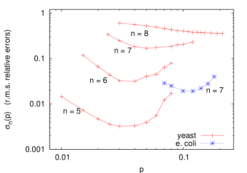
Figure 1: (color online) Root mean square relative errors of connected subgraph counts, Eq. (10), for the yeast ($n=5$ to $8$) and E. coli ($n=7$) networks. In most cases, clear minima indicate roughly the optimum value for $p$, with caveats as explained in the text. Each data point is based on $4\times 10^{9}$ generated subgraphs. Smaller values of $\sigma_{n}(p)$ indicate that the census for subgraphs with $n$ nodes is on average more precise.

As a first test, we compute the root mean square relative errors of the subgraph counts, averaged over all subgraphs of fixed size $n$. Let $\gamma_{n}$ be the number of different subgraphs of size $n$ found, and let $\Delta c_{G}$ be the error of the count for subgraph $G$. These errors were estimated by dividing the set of $M$ independent samples into bins, and estimating the fluctuations from bin to bin. Then

$$\sigma_{n}(p)=\left[{1\over\gamma_{n}}\sum_{j=1}^{\gamma_{n}}(\Delta c_{G_{j}}/{\hat{c}_{G_{j}}})^{2}\right]^{1/2}.$$ (10)

Smaller values of $\sigma_{n}(p)$ indicate that the subgraph census is on average more precise. Fig. 1 shows results for the yeast network, with various values of $p$ and $n$. Also shown are data for the E. coli network, for $n=7$. Each simulation used for this figure (i.e., each data point) involved $M=4\times 10^{9}$ generated clusters. Our first observation is that the results for E. coli are much more precise than those for yeast. This is mainly due to smaller hubs ($k_{\rm max}^{\rm e.coli}=36$, while $k_{\rm max}^{\rm yeast}=141$), so that much larger $p$ values footnote2 could be used. Also in all other aspects, our algorithm worked much better for the E. coli network than for yeast. Therefore we exhibit in the rest of this section only results for yeast, implying that whenever a test was positive for yeast, an analogous test had been made for E. coli with at least as good results.

Even with the large sample sizes used in Fig. 1, many $n=8$ subgraphs were found only once (in which case we set $\Delta c_{G_{j}}/{\hat{c}}_{G_{j}}=1$), which explains the high values of $\sigma_{8}(p)$. This is also why we do not show any data for $n>8$ in Fig. 1. The relative error $\sigma_{n}(p)$ for each $n<8$ shows a broad minimum as a function of $p$. The increase in $\sigma_{n}(p)$ at small $p$ is because of the paucity of different graphs being generated. This effect grows when $n$ increases, explaining why the minimum shifts to the right with increasing $n$. The increase of $\sigma_{n}(p)$ for large $p$, in contrast, comes from large fluctuations of weights for individual sampled graphs. When $p$ is large, the factor $(1-p)^{b-g}$ in Eq.(7) can also be large, particularly in the presence of strong hubs.

Unfortunately, if a subgraph is found only once, it is impossible to decide whether or not the frequency estimate is reliable. Even for strong outliers, when the frequency estimate is far too large, the formal error estimate cannot be larger than $\Delta c_{G}=O({\hat{c}}_{G})$. This underestimates the true statistical errors and is partially responsible for the fact that the curve for $n=8$ in Fig. 1 does not increase at large $p$ footnote3 .

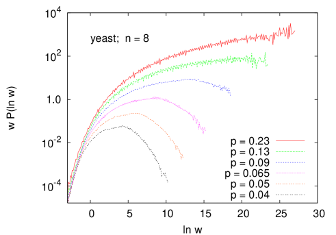
Figure 2: (color online) Histograms of $wP(\ln w)=w^{2}P(w)$ for connected $n=8$ subgraphs of the yeast network. Each curve corresponds to one run ($4\times 10^{9}$ generated subgraphs) with fixed value of $p$. Results are the more reliable, the further to the left is the maximum of the curve and the faster is the decrease of its tail at large $w$.

A more direct understanding of the decreasing performance at large $p$ comes from histograms of the (logarithms of) weight factors. Such histograms, for $n=8$ subgraphs in the yeast network, are shown in Fig. 2. From the results in Section II

$$w={2L\over nMk}p^{1-n}(1-p)^{g-b}$$ (11)

is the weight for a subgraph with $n$ nodes, $b$ boundary nodes, and $g$ growth nodes. The algorithm produces reliable estimates if $P(w)$ decreases for large $w$ faster than $1/w^{2}$, since averages (which are weighted by $w$) are then dominated by subgraphs that are well sampled. If, in contrast, $P(w)$ decreases more slowly, then the tail of the distribution dominates, and the results cannot be taken at face value grass-PERM . We observe from Fig. 2 that the data for $n=8$ is indeed reliable for $p<0.07$ only. The curve for $p=0.09$ in Fig. 2 also bends over at very large values of $w$, indicating that even for this $p$ our estimates should finally be reliable, when the sample sizes become sufficiently large. But this would require extremely large sample sizes.

As a last test we checked whether the estimates $\hat{c}_{G}$ are independent of $p$ as they should be. Fig. 3 shows the estimates obtained for $n=8$ subgraphs in the yeast network with $p=0.025$ and $p=0.07$ against those obtained with $p=0.04$. Clearly, the data cluster along the diagonal – showing that the estimates are basically correct. They scatter more when the counts are lower (i.e. in the lower left corner of the plot). The asymmetries in that region result from the fact that rarely occurring subgraphs are completely missed for $p=0.04$ and even more so for $p=0.025$, cutting off thereby the distributions at small ${\hat{c}}_{G}$. For larger counts, the estimates for $p=0.025$ are more precise than those for $p=0.07$. The latter show high weight “glitches” arising from the tail of $P(w)$ discussed earlier in this section.

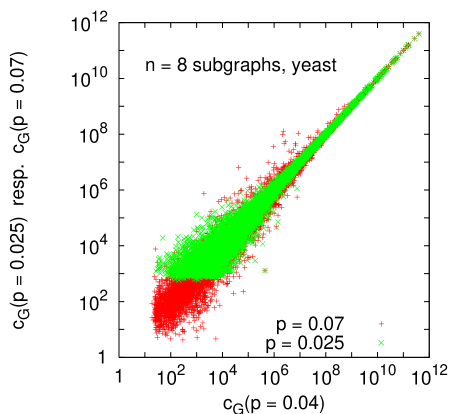
Figure 3: (color online) Scatter plots of ${\hat{c}}_{G}(p=0.025)$ and ${\hat{c}}_{G}(p=0.07)$ against ${\hat{c}}_{G}(p=0.04)$ for connected $n=8$ subgraphs of the yeast network. The clustering of the data along the diagonal indicates the basic reliability of the estimates, independent of the precise choice of $p$. Sample sizes were $4\times 10^{10}$ for $p=0.04$, $2.4\times 10^{10}$ for $p=0.025$, and $8\times 10^{9}$ for $p=0.07$. The latter two correspond to roughly the same CPU time.

For increasing $p$, the numbers $m_{G}$ of generated subgraphs of type $G$ increase of course (as the epidemic survives longer), so that average weights, defined as $\langle w_{G}\rangle={\hat{c}}_{G}M/m_{G}$, decrease. But this decrease is not uniform for all $G$. Rather, it is strongest for fully connected subgraphs ($\ell=n(n-1)/2$), and is weakest for trees. For the yeast network and $n=8$, e.g., $\langle w_{G}\rangle$ averaged over all trees decreases by a factor $\sim 18$ when $p$ increases from 0.025 to 0.085, while $\langle w_{G}\rangle$ averaged over all graphs with $\ell\geq 25$ decreases by a factor $\sim 1700$. Smaller values of $\langle w_{G}\rangle$ are preferable, as they imply smaller fluctuations. Thus it would be most efficient to use larger $p$ values for highly connected subgraphs, and smaller $p$ for tree-like subgraphs. Counting very highly connected subgraphs – where every node has a degree in the subgraph $\geq k_{0}$, say – is also made easier by first reducing the network to its $k$-core with $k=k_{0}$, and then sampling from the latter.

V Results

V.1 Characterization of the networks

As already stated, both networks as we use them are fully connected footnote . The E. coli network has 230 nodes and 695 links, while the yeast network has 2559 nodes and 7031 links. Both networks show strong clustering, as measured by the clustering coefficients watts-stro

$$C_{i}={2\over k_{i}(k_{i}-1)}\sum_{j<m}A_{jm}$$ (12)

where $k_{i}$ is the degree of node $i$ and the sum runs over all pairs of nodes linked directly to $i$. In Fig. 4 we show averages of $C_{i}$ over all nodes with fixed degree $k$. We see that $\langle C\rangle_{k}$ is quite large, but has a noticeably different dependence on $k$ for the two networks. While it decreases with $k$ for E. coli, it attains a maximum at $k\approx 15$ for yeast.

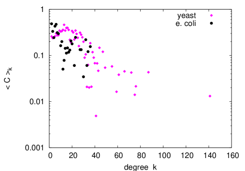
Figure 4: (color online) Average clustering coefficients for nodes with fixed degree $k$ plotted versus the degree, for the giant component of the yeast and E. coli protein interaction networks. While the clustering coefficient decreases with $k$ for E. coli, it attains a maximum at $k\approx 15$ for yeast.

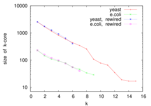
Figure 5: (color online) Sizes of the $k-$cores for the two networks, plotted against $k$. Notice that the $k-$cores for yeast contain a nearly fully connected cluster with 17 nodes. In addition to the core sizes for the original networks, the figure also shows average core sizes for rewired networks as discussed in section V C.

The unweighted average clustering ${\bar{C}}=N^{-1}\sum_{i=1}^{N}C_{i}$ is 0.1947 for yeast, and 0.2235 for E. coli. Due to the different behavior of $\langle C\rangle_{k}$, the ranking is reversed for the weighted averages

$$\langle C\rangle={\sum_{i=1}^{N}C_{i}k_{i}(k_{i}-1)\over\sum_{i=1}^{N}k_{i}(k_{i}-1)}={3n_{\Delta}\over 3n_{\Delta}+n_{\vee}},$$ (13)

where $n_{\Delta}$ is the number of fully connected triangles on the network and $n_{\vee}$ is the number of triads with two links (see newman_clust for a somewhat different formula). Numerically, this gives $\langle C\rangle=0.1948$ for yeast and 0.1552 for E. coli. This can be understood as a consequence of the fact that the relative frequency of fully connected triangles is higher in yeast than in E. coli: in yeast (E. coli) there are 6969 (478) triangles compared to 86291 (7805) triads with two links.

Associated with this difference are distinctions between the $k$-cores seidman of the two networks. Fig. 5 shows the sizes of the $k$-cores against $k$. We see that the yeast network contains non-empty cores with $k$ up to 15. Moreover, the core with $k=15$ has exactly 17 nodes. It is a nearly fully connected subgraph with just one missing link. All 17 proteins in this core are parts of the 26S proteasome which consists of 20 or 21 proteins mips ; sgd . All these proteins presumably interact very strongly with each other. When the interactions between the proteins within the 26S proteasome are taken out (the corresponding elements of the adjacency matrix are set to zero), the $k$-core with highest $k$ has $k=12$ and consists of 15 nodes. All its nodes correspond to proteins in the mediator complex of RNA polymerase II mips , which contains 20 proteins altogether. After eliminating all interactions between these, two 11-cores with respectively 13 and 14 nodes remain, the first corresponding to the 20S proteasome and the second corresponding to the RSC complex mips . Again these particular complexes have only a few more proteins than those contained within their largest $k$-cores, so they are very tightly bound together. All remaining complexes appear to be more loosely bound, so that much of the strong larger scale clustering in the yeast network (involving 7 - 10 nodes) can be traced to only a few tightly bound complexes. This has a big effect on the subgraph counts, as we shall see.

V.2 Trends in Subgraph counts

Subgraph counts ${\hat{c}}_{G}$ for the Escherichia coli and yeast networks, plotted against $n^{2}+2\ell$, are shown in Figs. 6 and 7. For large $n$ we see a very wide range, with counts varying between 1 and $>10^{8}$. In general, counts decrease with increasing number of links, i.e. trees are most frequent. This is a direct consequence of the fact that the networks are sparse. Even when $n$ and $\ell$ are fixed, the counts $c_{G}$ can range over six orders of magnitude (e.g. for yeast with $n=8$ and $\ell=17$).

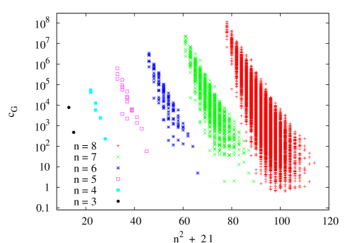
Figure 6: (color online) Counts for connected subgraphs with fixed topology and with $n\leq 8$ in the E. coli network, plotted against $n^{2}+2\ell$. The variable $n^{2}+2\ell$ is used to spread out the data, so that the dependence on both $n$ and $\ell$ (number of links) can be seen independently, without data points overlapping. For most of the points, the error bars are smaller than the sizes of the symbols.

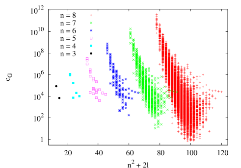
Figure 7: (color online) Counts for subgraphs with fixed topology and with $n\leq 8$ in the yeast network, plotted against $n^{2}+2\ell$ as in Fig. 6.

For the yeast network, there are clear systematic trends for the counts at fixed $n$ and $\ell$. The most frequent subgraphs are those with strong heterogeneity, i.e. with a large variation of the degrees (within the subgraph) of nodes, while the most rare are those with minimal variation. Fig. 8 shows the counts ${\hat{c}}_{G}$ for $n=8$ and with four different values of $\ell$ plotted against the variance of the degrees of the nodes within the subgraph,

$$\sigma^{2}={1\over n}\sum_{i=1}^{n}k_{i}^{2}-[{1\over n}\sum_{i=1}^{n}k_{i}]^{2}.$$ (14)

For all four curves we see a trend, where the count increases with $\sigma$, but hardly any trend like this is seen for the E. coli network (data not shown). The effect seen in the yeast data is probably related to the very strongly connected core in that network (see the last subsection). As we shall also see later in subsection D, subgraphs with high counts in yeast often have a tadpole form with a highly connected body (which is part of one of the densely connected complexes discussed in the last subsection) and a short tail attached to it. These cores may also be responsible for the main difference between Figs. 6 and 7, namely the strong representation of very highly connected (large $\ell$) subgraphs in the yeast network. Taking out all interactions within the 26S and 20S proteasomes, within the mediator complex and within the RSC complex reduces substantially the counts for highly connected subgraphs. The count for the complete $n=7$ subgraph, e.g., is reduced in this way from $25,164\pm 68$ to $682\pm 23$. The removal of interactions within the 26S proteasome makes by far the biggest contribution.

Figure 8: (color online) Counts for $n=8$ subgraphs of the yeast network with $\ell=7,10,13,$ and $18$, plotted against the variance of the node degrees within the subgraphs, as given by Eq. 14. Zero variance means that all nodes have exactly the same degree, whereas a higher variance indicates that the nodes differ more widely. Typically, subgraphs with more variation in their nodes (and thus with larger $\sigma^{2}$) have higher counts than those for which the degrees within the subgraph are more uniform.

V.3 Zipf plots

In baskerville it was found that “Zipf plots” (subgraph counts vs. rank) in the E. coli network exhibit power law behavior, whose origin is not yet understood. The essential difference between the subgraph counts in baskerville and in the present paper is that we sample only connected subgraphs, while all subgraphs with given $n$ were ranked in baskerville . Also, noting that disconnected subgraphs are more likely to be sampled than connected ones when picking nodes at random (due to the sparsity of the networks), we can go to much higher ranks for the connected subgraphs.

Zipf plots for connected subgraphs in the E. coli network are shown in Fig. 9. Each curve is based on $4\times 10^{9}$ to $10^{10}$ generated subgraphs. Each is strongly curved, suggesting that there are no power laws – at least for subgraph sizes where we obtain reasonable statistics for the census. The curves show less curvature for larger $n$, but this is a gradual effect. It seems that the scaling behavior found in baskerville was mainly due to the presence of disconnected graphs, although it is not immediately obvious why those should give scale-free statistics either. In addition, the right hand tails of the Zipf plots in baskerville were cut off because of substantially lower statistics. In our case, apparently sharp cutoffs in the counts are observed for ranks $\approx 1.08\times 10^{4}$ for $n=8$, $\approx 2.1\times 10^{5}$ for $n=9$, and $\approx 2.9\times 10^{6}$ for $n=10$. For $n\leq 9$ these are close to the total number of different connected subgraphs briggs , suggesting that we have fairly complete statistics. For $n=10$ the cutoff is more affected by lack of statistics, but it is still within a factor of four of the upper limit.

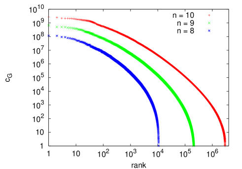
Figure 9: (color online) “Zipf” plots showing the counts for individual connected subgraphs with fixed $n$, plotted against their rank. Data are for the E. coli network.

V.4 Null model comparison and motifs

One of the most striking results of baskerville was that most large subgraphs were either strong motifs or strong anti-motifs. However, this finding was based on rather limited statistics and on a single protein interaction network. One of the purposes of the present study is to test this and other results of baskerville with much higher statistics and for a larger network, the protein interaction network of yeast.

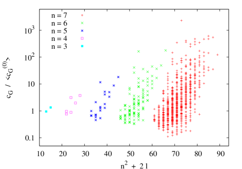
Figure 10: (color online) Ratios between the count estimates $\hat{c}_{G}$ for connected subgraphs in the E. coli network, and the corresponding average counts $\langle\hat{c}^{(0)}_{G}\rangle$ in rewired networks. The data are plotted against $n^{2}+2\ell$, again to spread the points out conveniently. Most error bars are smaller than the symbols.

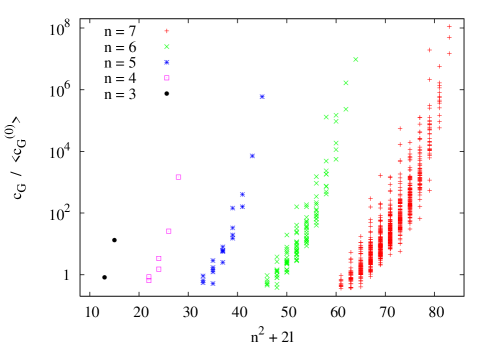
Figure 11: (color online) Same as Fig. 10, but for the yeast network. Notice that most data points for large $n$ and $\ell$ are missing. Indeed, for $n=7$ all (!) data points with $\ell>16$ are missing, because no such subgraphs were found in the rewired ensemble.

To define a motif requires a null model. We take this to be the ensemble of networks with the same degree sequence, obtained by the rewiring method. The average subgraph counts in the null ensemble are denoted as $\langle c_{G}^{(0)}\rangle$. In Figs. 10 and 11 we plot the ratios $c_{G}/\langle c_{G}^{(0)}\rangle$ against the variable $n^{2}+2\ell$ for each connected subgraph that was sampled both in the original graph and in at least one of the rewired graphs. The error bars, which include both statistical errors from sampling and the ensemble fluctuations of the null model estimated from several hundred rewired networks, are for most points smaller than the symbols. A subgraph is a motif (anti-motif), if this ratio is significantly larger (smaller) than 1. Notice that motifs do not in general occur particularly frequently in the original network. Even without rigorous estimates to estimate significance, it is clear that most densely connected subgraphs are motifs in the yeast network. The fact that trees or subgraphs with few loops tend to be anti-motifs might not be so evident from Fig. 11, since the ratios for trees and tree-like graphs are close to one. Thus we have to discuss significance more formally.

V.4.1 $Z$-scores

Usually baskerville , the significance of a motif (or anti-motif) is measured by its $Z$-score

$$Z={c_{G}-\langle c_{G}^{(0)}\rangle\over\sigma_{G}^{(0)}}\;,$$ (15)

where $\sigma_{G}^{(0)}$ is the standard deviation of $c_{G}$ within the null ensemble. A subgraph is a motif (anti-motif), if $Z\gg 1$ ($Z\ll-1$).

The eight strongest motifs with $n=7$ in the E. coli network according to this definition are shown in Fig. 12, together with their $Z$-values. To name the strongest motifs in the yeast network is less straight forward, since many subgraphs did not show up in any rewired network at all. Assuming for those subgraphs $\sigma_{G}^{(0)}=\langle c_{G}^{(0)}\rangle=0$ would give $Z=\infty$. Rough lower bounds on $Z$ are obtained for them by assuming that $\langle c_{G}^{(0)}\rangle<1/R$ and $\sigma_{G}^{(0)}<1/\sqrt{R}$, where $R$ is the number of rewired networks that were sampled, giving $Z\geq c_{G}\sqrt{R}$. Some of the strongest motifs in the yeast network, together with their estimated $Z$-scores, are shown in Fig. 13. Note that no $n=7$ graphs with $\ell>16$ were found in any of the realizations of the null model, while they were all found in the real yeast network. Hence these are all strong motifs. Those motifs in Fig. 13 for which only lower bounds for the $Z$-score are given are the most frequent in the real network, hence they have the highest lower bound. It was pointed out in spirin ; ispolatov that cliques (complete subgraphs) are in general very strong motifs. In yeast, the $n=7$ clique (with $\ell=21$) is indeed a very strong motif, but it does not have the largest lower bound on the $Z$-score. In comparison, anti-motifs have rather modest $Z$-scores. The strongest anti-motif with $n=7$ has $Z=-32.9$ ($Z=-24.7$) for E. coli (yeast).

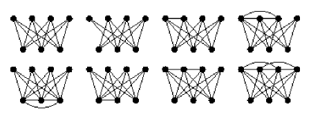
Figure 12: The eight strongest motifs with $n=7$ in the E. coli protein interaction network. These tend to be almost bipartite graphs, and many pairs of nodes are linked to the same set of neighbors. Their $Z$-scores, in order from left to right, first then second row, are: $2.9\times 10^{4},932,885,648,595,532,516$ and 377. Their estimated frequencies in the original E. coli network are, in the same order: $20936\pm 8,161521\pm 63,8312\pm 5,1331\pm 2,838\pm 2,5985\pm 5,5165\pm 4,$ and $519\pm 1$.

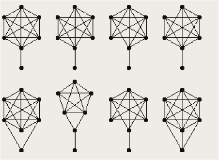
Figure 13: Eight very strong motifs with $n=7$ for the yeast protein interaction network. These tend to be almost complete graphs with a single dangling node. Four of these graphs were not seen in any realization of the null model, so only lower bounds on their $Z$-scores can be given. From left to right, first then second row, the estimated $Z$-scores are: $>3\times 10^{7},9\times 10^{5},>8\times 10^{6},5\times 10^{5},>4\times 10^{6},3\times 10^{5},2.5\times 10^{5}$, and $>1.5\times 10^{6}$. Estimated frequencies are, in the same order: $6.68(1)\times 10^{5},9.27(5)\times 10^{4},1.76(1)\times 10^{5},4.84(1)\times 10^{5},7.78(2)\times 10^{4},3.13(6)\times 10^{5},1.38(1)\times 10^{5}$, and $3.35(1)\times 10^{4}$.

With $Z$-values up to $10^{7}$ and more, as in Fig. 13, the motivation for using $Z$-scores becomes suspect. On the one hand, the null model is clearly unable to describe the actual network, and has to be replaced by a more refined null model. This will be done in a future paper newpaper . On the other hand, it suggests to use instead a $Z$-score based on logarithms of counts,

$$Z_{\rm log}={\log c_{G}-\langle\log c_{G}^{(0)}\rangle\over\sigma_{\log,G}^{(0)}}\;,$$ (16)

where $\sigma_{\log,G}^{(0)}$ is the standard deviation of $\log c_{G}^{(0)}$. An advantage of Eq.(16) would be that it suppresses $|Z|$ for motifs, but enhances $|Z|$ for anti-motifs.

In general, strong yeast motifs have a tadpole structure with a complete or almost complete body, and a tail consisting of a few nodes with low degree. This agrees nicely with our previous observation that frequently occurring subgraphs in the yeast network have strong heterogeneity in the degrees of their nodes. In contrast, strong E. coli motifs with not too many loops are all based on a 4-3 or 5-2 bipartite structure. When the number of loops increases, strictly bipartite structures are impossible, but the tendency towards these structures is still observed.

Whether we use $Z$-scores or the ratio $C_{G}/C_{G}^{(0)}$ to identify motifs makes very little difference. Using either criterion, the strengths of the strongest motifs skyrocket with subgraph size. This is most dramatically apparent for the yeast network. Indeed, correlations between $Z$-scores of individual graphs in the yeast and E. coli networks (data not shown) are much weaker than correlations between count ratios. The latter are shown in Fig. 14 for $n=7$ subgraphs.

V.4.2 Twinning versus Clustering

Another characteristic feature of strong motifs in the E. coli network is the tendency for ‘twin’ nodes. We call two nodes in a subgraph twins if they are connected to the same set of neighbours in the subgraph. Otherwise said, nodes $i$ and $k$ are twins, iff the $i$-th and $k$-th rows of the subgraph adjacency matrix are identical. Notice that twin nodes can be created most naturally by duplicating genes. We found that subgraphs with many pairs of twin nodes are in general also motifs in the yeast network, but they do not stand out spectacularly from the mass of other motifs. They could be the ‘genuine’ motifs also for yeast, but only a better null model where all subgraphs actually occur with reasonable frequency would be able to prove or disprove this.

In Fig. 14 we also indicated the dependence on the number $n_{\rm twin}$ of pairs of twin nodes, by marking subgraphs with $n_{\rm twin}>3$ ($n_{\rm twin}>1)$ by bullets (asterisks). We see that all strong motifs in E. coli have multiple pairs of twin nodes. These subgraphs tend to be also motifs of comparable strength in yeast – the bullets in Fig. 14 tend to cluster on the diagonal $[c_{G}/\langle c_{G}^{(0)}\rangle]_{\it E.~{}coli}=[c_{G}/\langle c_{G}^{(0)}\rangle]_{yeast}$. However, there are even stronger motifs in yeast that have no twin nodes. These graphs are typically much weaker motifs or not motifs at all in E. coli.

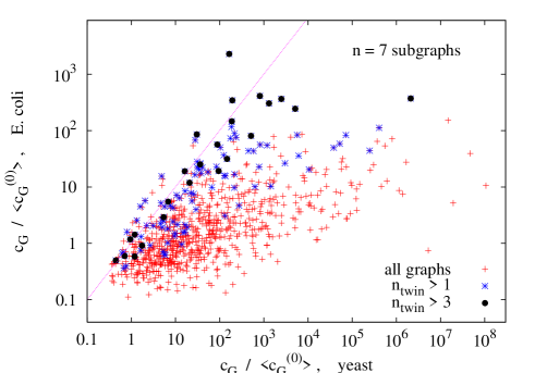
Figure 14: (color online) Count ratios $c_{G}/\langle c_{G}^{(0)}\rangle$ for individual subgraphs in the E. coli network, plotted against the count ratio for the same subgraph in the yeast network. To highlight the dependence on the number of twin nodes in the subgraph, subgraphs with $n_{\rm twin}>1\;(n_{\rm twin}>3)$ are marked by asterisks (bullets). Whereas almost all ratios are much higher in the yeast network, this is noticeably less true for subgraphs containing more than three pairs of twin nodes. These tend to fall on the diagonal indicated by the dashed line.

As we have already indicated, many of the strong motifs in yeast seem to be related to a few densely connected complexes such as those discussed in subsection A. They are either part of their cores, or they have most of their nodes in the core, with one or two extra nodes forming the tail of what looks like a tadpole. This effect is even more pronounced for $n=8$ subgraphs. For instance, the three most frequent subgraphs with $n=8$ and $\ell=17$ all contained a 6-clique and two nodes connected to it either in chain or in parallel. None of them occurred even in a single rewired network.

The situation is different for the E. coli network. There, the three most frequent graphs with 8 nodes and 17 edges also have a tadpole structure, few twin nodes, and low bipartivity. But they are not very strong motifs since they occur also frequently in the rewired networks. The three strongest motifs with $n=8$ and $\ell=17$, in contrast, have many twin pairs and high bipartivity. They have slightly lower counts (by factors 2-4), but occur much more rarely in the rewired networks.

Figure 15: (color online) Counts $c_{G}$ resp. $\langle c_{G}^{(0)}\rangle$ for individual subgraphs in the Escherichia coli network, plotted against counts for the same subgraph in the yeast network. It can be seen that the two rewired networks are much more similar (display higher correlation) than the original networks.

V.4.3 Effects of Rewiring on Differences between Networks

Finally, Fig. 15 shows counts for individual subgraphs in the E. coli network against counts for the same subgraph in yeast. This is done for all four combinations of original and rewired networks. We see that the correlation is strongest when we compare rewired networks of E. coli to rewired networks of yeast. This is not surprising. It means that a lack of correlations is mostly due to special features of one network which are not shared by the other. Rewiring eliminates most of these features. The other observation is that rewiring in general reduces further the counts for subgraphs which are already rare in the original networks. This is mainly due to the fact that such subgraphs are relatively densely connected, and appear in the original networks only because of the strong clustering. This effect is more pronounced for yeast than for E. coli, because it is more sparse and has more densely connected clusters/complexes.

VI Discussion

In this paper we have presented an algorithm for sampling connected subgraphs uniformly from large networks. This algorithm is a generalization of algorithms for sampling lattice animals, hence we refer to it as a “graph animal algorithm” and to the connected subgraphs as “graph animals”. It allowed us to obtain high statistics estimates of subgraph censuses for two protein interaction networks. Although the graph animal algorithm worked well in both cases, the analysis of the smaller network (E. coli) was much easier than that of the bigger (yeast). This was not so much because of the sheer size of the latter (the yeast network has about ten times more nodes and links than the E. coli network), but was mainly caused by the existence of stronger hubs. Indeed, the presence of hubs places a more stringent limitation on the method than the size of the network.

One of the main results is that many subgraph frequency counts are hugely different from those in the most popular null model, which is the ensemble of networks with fixed degree sequence. Based on a comparison with this null model, most subgraphs with size $\geq 6$ in both networks would be very strong motifs or anti-motifs. This clearly shows that alternative null models are needed which take clustering and other effects into account.

While this was not very surprising (hints of it had been found in previous analyses), a more surprising result is the fact that the dominant motifs in the two protein interaction networks show very different features. Most of these seem to be related to the densely connected cores of a small number of complexes in the yeast network, which have no parallels in the E. coli network and which strongly affect the subgraph census. Further studies are needed to disentangle these effects from other – possibly biologically more interesting – effects.

Finally, a feature with likely biological significance is the dominance of subgraphs with many twin nodes. These are nodes which share the same list of linked neighbors within the subgraph. They correspond to proteins which interact with the same set of other proteins. The most natural explanation for them is gene duplication. Connected to this is a preference for (approximately) bipartite subgraphs. These two features are very clearly seen in the E. coli network, much less so in yeast. But it would be premature to conclude that gene duplication was evolutionary more important in E. coli than in yeast. It is more likely that its effect is just masked in the yeast network by other effects, most probably by the densely connected complexes and other clustering effects which do not show up to the same extent in E. coli.

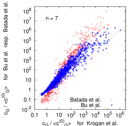
Figure 16: (color online) Count ratios $c_{G}/\langle c_{G}^{(0)}\rangle$ for individual subgraphs in the yeast networks of Refs. bu ; batada , plotted against counts for the same subgraph in the network of yeast . If all three networks were identical, all points should lie on the diagonal (indicated by the straight dashed line), whereas in fact systematic deviations are observed.

Up to now, we know very little about the biological significance of our findings. One main avenue of further work could be to relate our results on subgraph abundances in more detail to properties of the network that are associated with biological function. Another important problem is the comparison between network reconstructions which supposedly describe the same or similar objects. There exist, e.g., a large number of published protein-protein interaction networks for yeast. Some were obtained by means of different experimental techniques, either with conventional or with high throughput methods, while others were obtained by comprehensive literature compilations. In a preliminary step, we compared three such networks: The network obtained by Krogan et al. yeast that was studied above, a somewhat older network downloaded from pajek and attributed to Bu et al. bu , and the ‘high confidence’ (HC) network of Batada et al. batada . The latter is the most recent. It was obtained by extracting the most reliable interactions from a vast data base which includes the data of both Bu et al. and Krogan et al.. In Fig. 16 we plot the ratios between the actual counts and the average counts in rewired networks for Bu et al. and for the HC data set against the analogous ratios for the Krogan et al. networks. If the three data sets indeed describe the same yeast network – as they purport to do, within experimental uncertainties – the points should all fall onto the diagonal. Instead, we see systematic deviations. Surprisingly, these deviations are much stronger between the Krogan et al. and the HC networks than between the Krogan et al. and the Bu et al. networks. Clarifying these and other systematic irregularities should give valuable insight into the strengths and weaknesses of the methods used in constructing the networks as well as their biological reliability, and should lead to improved methods for network reconstruction.

In the present paper we have only dealt with undirected networks. The basic sampling algorithm works equally well for directed networks. The main obstacle in applying our methods to the latter is the huge number of directed subgraphs, even for relatively small sizes. Nevertheless, we will present an analysis of directed networks in forthcoming work, as well as applications to other undirected networks.

Acknowledgements: We thank Gabriel Musso for valuable information on the yeast network.

References

- (1) C. Faloutsos, M. Faloutsos, and P. Faloutsos, ACM SIGCOMM Computer Communication Review 29, 251 (1999).
- (2) A.-L. Barabasi and R. Albert, Science 286, 509 (1999).
- (3) B. Bollobas, Random Graphs (Academic Press, London 1985).
- (4) M.E.J. Newman, SIAM Review 45, 167 (2003).
- (5) D.J. Watts and S.H. Strogatz, Nature 393, 440 (1998).
- (6) M.E.J. Newman, Phys. Rev. E 64, 016131 (2001).
- (7) E. Ravasz, L. Somera, D.A. Mongru, Z.N. Oltvai, and A.-L. Barabási, Science 297, 1551 (2002).
- (8) M.E.J. Newman and M. Girvan, Phys. Rev. E 69, 026113 (2004).
- (9) E. Ziv, M. Middendorf, and C. Wiggins, Phys. Rev. E 71, 046117 (2005).
- (10) M. Rosvall and C.T. Bergstrom, Proc. Nat. Acad. Sci. U.S.A. 104, 7327 (2007).
- (11) K. Klemm and P.F. Stadler, Phys. Rev. E 73, 025101(R) (2006).
- (12) S. Milgram, Psychology Today 2, 60 (1967).
- (13) E. Estrada and J.A. Rodríguez-Velázquez, Phys. Rev. E 72, 046105 (2005); E. Estrada, J. Proteome Res. 5, 2177 (2006).
- (14) R. Milo, S. Shen-Orr, S. Itzkovitz, N. Kashtan, D. Chklovskii, and U. Alon, Science 298, 824 (2002).
- (15) S. Shen-Orr, R. Milo, S. Managan, and U. Alon, Nat. Genet. 31, 64 (2002).
- (16) A. Vásquez, R. Dobrin, D. Sergi, J.-P. Eckmann, Z.N. Oltvai, and A.-L. Barabasi, Proc. Nat. Acad. Sci. U.S.A. 101, 17940 (2004).
- (17) N. Kashtan, S. Itzkovitz, R. Milo, and U. Alon, Phys. Rev. E 70, 031909 (2004).
- (18) J. Besag and P. Cliffors, Biometrica 76, 633 (1989).
- (19) S. Maslov and K. Sneppen, Science 296, 910 (2002).
- (20) M. Middendorf, E. Ziv and C. H. Wiggins, Proc. Natl. Acad. Sci. U.S.A. 102, 3192 (2005).
- (21) P. Mahadevan, D. Krioukov, K. Fall, and A. Vahdat, “A Basis for Systematic Analysis of Network Topologies”, preprint arXiv/cs.NI/0605007v2 (2006).
- (22) J. Park and M. E. J. Newman, Phys. Rev. E 68, 026112 (2003).
- (23) J. Park and M. E. J. Newman, Phys. Rev. E 70, 066117 (2004).
- (24) J. Foster, D. Foster, P. Grassberger and M. Paczuski, e-print cond-mat/0610446 (2006).
- (25) A. Clauset, C. Moore, and M. E. J. Newman, e-print physics/0610051 (2006).
- (26) K. Briggs, http://keithbriggs.info/cgt.html (2006).
- (27) J.U. Köbler and J.T. Schöning, The Graph Isomorphism Problem: Its Structural Complexity (Birkhauser, Boston 1993).
- (28) J.-L. Faulon, J. Chem. Inf. Comput. Sci. 38, 432 (1998).
- (29) J. Torán, FOCS 180 (2000).
- (30) For the “nauty” program of B. MacKay, see http://cs.anu.edu.au/people/bdm/nauty/
- (31) K. Baskerville and M. Paczuski, Phys. Rev. E 74, 051903 (2006).
- (32) N. Kashtan, S. Itzkovitz, R. Milo, and U. Alon, Bioinformatics 20, 1746 (2004).
- (33) V. Spirin and L.A. Mirny, Proc. Nat. Acad. Sci. U.S.A. 100, 12123 (2003).
- (34) R.C. Read, Canad. J. Math. 14, 1 (1962).
- (35) I. Jensen, J. Stat. Phys. 102, 865 (2001).
- (36) S. Redner, J. Statist. Phys. 29, 309 (1982).
- (37) D. Stauffer, Phys. Rev. Lett. 41, 1333 (1978).
- (38) R. Dickman and W.C. Schieve, J. Physique 45, 1727 (1984).
- (39) E J Janse van Rensburg and N Madras, J. Phys. A: Math. Gen. 25 303 (1992).
- (40) P. Leath, Phys. Rev. B 14, 5046 (1976).
- (41) H.-P. Hsu, W. Nadler, and P. Grassberger, J. Phys. A: Math. Gen. 38, 775 (2005); e-print cond-mat/0408061 (2004).
- (42) K. Baskerville et al., in preparation.
- (43) P. Grassberger, H. Frauenkron, and W. Nadler, PERM: A Monte Carlo Strategy for Simulating Polymers and other Things, in “Monte Carlo Approach to Biopolymers and Protein Folding”, eds. P. Grassberger et al. (World Scientific, Singapore 1998); arXiv:cond-mat/9806321 (1998).
- (44) C.M. Care, Phys. Rev. E 56, 1181 (1997); C.M. Care and R. Ettelaie, Phys. Rev. E 62, 1397 (2000).
- (45) S. Redner, J. Phys. A: Math. Gen. 12, L239 (1979).
- (46) G. Butland et al., Nature 433, 531 (2005); http://www.cosin.org.
- (47) N.J. Krogan et al., Nature 440, 637 (2006).
- (48) The networks given in ecoli ; yeast are not connected. In the present paper we used only their largest connected components.
- (49) D. Stauffer and A, Aharony, An Introduction to Percolation Theory, 2nd Ed. (Taylor and Francis, London, 1994).
- (50) P. Grassberger, J. Phys. A: Math. Gen. 26, 1023 (1993).
- (51) D. Mollison, J. R. Statist. Soc. B 39, 283 (1977).
- (52) P. Grassberger, Mathematical Biosciences 63, 157 (1983).
- (53) The On-Line Encyclopedia on Integer Sequences, http://www.research.att.com/ njas/sequences (AT&T Labs, 2006).
- (54) R. Pastor-Satorras and A. Vespignani, Phys. Rev. Lett. 86, 3200 (2001).
- (55) We might try to estimate the optimal by the threshold for an infinite SIR epidemic on an infinite tree like network with the same degree distribution, pastor . For the two networks considered in this paper, this would give , , i.e. a much smaller difference in the optimal values. One reason why this is not observed might be the very strong clustering, in particular in the yeast data, which is neglected in this argument.
- (56) Another reason why no minimum appears in the curve is that we kept the number of generated clusters fixed, not CPU time. Since larger values also imply larger clusters in average, the CPU time per cluster increases sharply for larger .
- (57) P. Grassberger and W. Nadler, “Go with the winners”-Simulations, in “Computational Statistical Physics: From Billards to Monte Carlo”, eds. K.H. Hoffmann et al. (Springer, Heidelberg 2000); arXiv:cond-mat/0010265 (2000).
- (58) S.B. Seidman, Social Networks 5, 269 (1983).
-
(59)
MIPS data base:
http://mips.gsf.de/genre/proj/yeast/Search/Catalogs/catalog.jsp. -
(60)
SGD data base:
http://www.yeastgenome.org/cgi-bin/GO/go.pl?. - (61) I. Ispolatov, P.L. Krapivsky, I. Mazo, and A. Yuryev, New Journal of Physics 7, 145 (2005).
- (62) http://vlado.fmf.uni-lj.si/pub/networks/data/bio/Yeast/Yeast.htm.
- (63) D. Bu et al., Nucleic Acids Res. 31, 2443 (2003).
- (64) N.N. Batada et al., PLoS Biology 4, 1720 (2006).