Network-based analysis of stochastic SIR epidemic models with random and proportionate mixing

Abstract

In this paper, we outline the theory of epidemic percolation networks and their use in the analysis of stochastic SIR epidemic models on undirected contact networks.  We then show how the same theory can be used to analyze stochastic SIR models with random and proportionate mixing.  The epidemic percolation networks for these models are purely directed because undirected edges disappear in the limit of a large population.  In a series of simulations, we show that epidemic percolation networks accurately predict the mean outbreak size and probability and final size of an epidemic for a variety of epidemic models in homogeneous and heterogeneous populations.  Finally, we show that epidemic percolation networks can be used to re-derive classical results from several different areas of infectious disease epidemiology.  In an appendix, we show that an epidemic percolation network can be defined for any time-homogeneous stochastic SIR model in a closed population and prove that the distribution of outbreak sizes given the infection of any given node in the SIR model is identical to the distribution of its out-component sizes in the corresponding probability space of epidemic percolation networks.  We conclude that the theory of percolation on semi-directed networks provides a very general framework for the analysis of stochastic SIR models in closed populations.

1 Introduction

In an important paper, M. E. J. Newman studied a network-based Susceptible-Infectious-Removed (SIR) epidemic model in which infection is transmitted through a network of contacts between individuals [1].  The contact network itself was a random undirected network with an arbitrary degree distribution of the form studied by Newman, Strogatz, and Watts [2].  Given the degree distribution, these networks are maximally random.  Thus, they have no small loops in the limit of a large population [2, 3, 4].

In the SIR model from [1], the probability that an infected node $i$ makes infectious contact with an adjacent node $j$ is given by $T_{ij}=1-\exp(-r_{i}\beta_{ij})$, where $\beta_{ij}$ is the rate of infectious contact from $i$ to $j$ and $r_{i}$ is the time that $i$ remains infectious.  (In this paper, we use infectious contact to mean a contact that results in infection if and only if the recipient is susceptible.)  The recovery period $r_{i}$ is a random variable with the cumulative distribution function (cdf) $F(r)$ and the infectious contact rate $\beta_{ij}$ has the cdf $F(\beta)$.  The infectious periods for all individuals are independent and identically distributed (iid) and the infectious contact rates for all ordered pairs of individuals are iid.

This model can be analyzed by mapping the SIR model onto a semi-directed network that we call the epidemic percolation network [5].  Since the distribution of recovery periods for all nodes and the joint distribution of contact rates for all pairs of connected nodes are defined a priori, all relevant transmission probabilities can be determined by assigning the infectious periods and contact rate pairs before an epidemic begins.  Starting from the contact network, a single realization of the epidemic percolation network can be generated as follows:

1. Choose a recovery period $r_{i}$ for every node $i$ and choose a contact rate $\beta_{ij}$ for every ordered pair of connected nodes $i$ and $j$ in the contact network.

2. For each pair of connected nodes $i$ and $j$ in the contact network, convert the undirected edge between them to a directed edge from $i$ to $j$ with probability

   $$(1-e^{-r_{i}\beta_{ij}})e^{-r_{j}\beta_{ji}},$$

   to a directed edge from $j$ to $i$ with probability

   $$e^{-r_{i}\beta_{ij}}(1-e^{-r_{j}\beta_{ji}}),$$

   and erase the edge completely with probability $\exp(-r_{i}\beta_{ij}-r_{j}\beta_{ji})$.  The edge remains undirected with probability

   $$(1-e^{-r_{i}\beta_{ij}})(1-e^{-r_{j}\beta_{ji}}).$$

The epidemic percolation network is a semi-directed network that represents a single realization of the infectious contact process for each connected pair of nodes, so $4^{m}$ possible epidemic percolation networks exist for a contact network with $m$ edges.  The probability of each network is determined by the underlying SIR model.  The epidemic percolation network is very similar to the locally dependent random graph defined by Kuulasmaa [6] for an epidemic on a $d$-dimensional lattice, with two important differences: First, the underlying structure of the contact network is not assumed to be a lattice.  Second, we replace pairs of (occupied) directed edges between two nodes with a single undirected edge.  The idea of the epidemic percolation network is also similar to the idea of forward and backward branching processes, which have been used to derive the probability and final size of an epidemic, respectively, in SIR models with independent infectiousness and susceptibility [7].  The epidemic percolation network can be thought of as a simultaneous mapping of the forward and backward branching processes that generalizes to models with arbitrary joint distributions of infectiousness and susceptibility.  (The relationship between epidemic percolation networks and branching processes is discussed further in Section 5.1.)

In the Appendix, we define epidemic percolation networks for a very general time-homogeneous stochastic SIR epidemic model (which includes network-based models and models with random and proportionate mixing as special cases) and prove that the size distribution of outbreaks starting from node $i$ is identical to the distribution of its out-component sizes in the corresponding probability space of percolation networks.  Because of this equality of distribution, epidemic percolation networks can be used to analyze a much more general class of epidemic models than that defined in the Introduction.  In this paper, we show how they can be used to analyze stochastic SIR epidemic models with random or proportionate mixing.

1.1 Structure of semi-directed networks

In this subsection, we review the structure of directed and semi-directed networks as discussed in [3, 4, 8, 9].  Reviews of the structure and analysis of undirected and purely directed networks can be found in [10, 11, 12, 13].

The indegree and outdegree of node $i$ are the number of incoming and outgoing directed edges incident to $i$.  Since each directed edge is an outgoing edge for one node and an incoming edge for another node, the mean indegree and outdegree of a semi-directed network are equal.  The undirected degree of node $i$ is the number of undirected edges incident to $i$.

A component is a maximal group of connected nodes.  The size of a component is the number of nodes it contains and its relative size is its size divided by the total size of the network.  There are four types of components in a semi-directed network.

The out-component of node $i$ includes $i$ and all nodes that can be reached from $i$ by following a series of edges in the proper direction (undirected edges are bidirectional).  The in-component of node $i$ includes $i$ and all nodes from which $i$ can be reached by following a series of edges in the proper direction.  By definition, node $i$ is in the in-component of node $j$ if and only if $j$ is in the out-component of $i$.  Therefore, the mean size of in- and out-components in any semi-directed network must be equal.

The strongly-connected component of a node $i$ is the intersection of its in- and out-components; it is the set of all nodes that can be reached from node $i$ and from which node $i$ can be reached.  All nodes in a strongly-connected component have the same in-component and the same out-component.  The weakly-connected component of node $i$ is the set of nodes that are connected to $i$ when the direction of the edges is ignored.

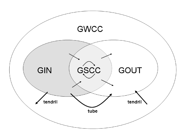
Figure 1: “Bowtie” diagram showing the giant components, tendrils, and tubes of a supercritical semi-directed network.  Adapted from Broder et al. [8] and Dorogovtsev et al. [9].

For giant components, we use the definitions given in [9, 14].  Giant components are so called because they have asymptotically positive relative size in the limit of a large population.  All other components are ”small” in the sense that they have asymptotically zero relative size.  There are two phase transitions in a semi-directed network: One where a unique giant weakly-connected component (GWCC) emerges and another where unique giant in-, out-, and strongly-connected components (GIN, GOUT, and GSCC) emerge.  The GWCC contains the other three giant components.  The GSCC is the intersection of the GIN and the GOUT, which are the common in- and out-components of nodes in the GSCC.  Tendrils are components in the GWCC that are outside the GIN and the GOUT.  Tubes are directed paths from the GIN to the GOUT that do not intersect the GSCC.  All tendrils and tubes are small components.  A schematic representation of these components is shown in Figure 1.

1.2 Epidemic percolation networks and epidemics

An outbreak begins when one or more nodes are infected from outside the population.  These are called imported infections.  The final size of an outbreak is the number of nodes that are infected before the end of transmission, and its relative final size is its final size divided by the total size of the network.  The nodes infected in the outbreak can be identified with the nodes in the out-components of the imported infections.  This identification is made mathematically precise in the Appendix.

We define a self-limited outbreak to be an outbreak whose relative final size approaches zero in the limit of a large population.  An epidemic is an outbreak whose relative final size is positive in the limit of a large population.  For many SIR epidemic models (including the one in the Introduction), there is an epidemic threshold: The probability of an epidemic is zero below the epidemic threshold and the probability and relative final size of an epidemic are positive above the epidemic threshold [1, 15, 7, 16].

If all out-components in the epidemic percolation network are small, then only self-limited outbreaks are possible.  If the epidemic percolation network contains a GSCC, then any infection in the GIN will lead to the infection of the entire GOUT.  Therefore, the epidemic threshold corresponds to the emergence of the GSCC in the epidemic percolation network.  For any set of imported infections, the probability of an epidemic is equal to the probability that at least one imported infection occurs in the GIN.  For any finite set of imported infections, the relative final size of an epidemic is asymptotically equal to the proportion of the network contained in the GOUT.  Although some nodes outside the GOUT may be infected (e.g. tendrils and tubes), they will constitute a finite number of small components whose total relative size is asymptotically zero.

This argument can be extended to epidemic percolation networks for heterogeneous populations.  The size distribution of outbreaks starting from an initial infection in any given node $i$ is equal to the distribution of the out-component sizes of node $i$ in the probability space of epidemic percolation networks.  In the limit of a large population, the probability that the infection of node $i$ causes an epidemic is equal to the probability that $i$ is in the GIN and the probability that $i$ is infected in an epidemic is equal to the probability that $i$ is in the GOUT.  Note that the size distribution of outbreaks and the probability of an epidemic can depend on the initial infection(s), but the relative final size of an epidemic does not.

1.3 Random and proportionate mixing

In this paper, we show how epidemic percolation networks can be used to analyze stochastic SIR epidemic models with random or proportionate mixing.  Methods exist to calculate the final size distribution of epidemics for such models in a population of size $n$, but they require solving a recursive system of $n$ equations [15, 17].  We will show how the size distribution of outbreaks, the epidemic threshold, and the probability and relative final size of a large epidemic can be calculated in the limit of large $n$ by solving a much simpler set of equations.  These methods also generalize more easily to heterogeneous populations.  We will show that these methods are equivalent to branching processes when the indegree and outdegree of the epidemic percolation network are independent, and we will use them to re-derive classical results from several areas of theoretical infectious disease epidemiology.

The rest of the paper is organized as follows: In Section 2, we find the degree distributions of the epidemic percolation networks corresponding to SIR models with random and proportionate mixing.  In Section 3, we review the use of probability generating functions to analyze semi-directed networks and show how these simplify in the case of purely directed networks.  In Section 4, we present a series of simulations to show that epidemic percolation networks accurately predict the mean outbreak size and the probability and final size of an epidemic for SIR models with random and proportionate mixing.  In Section 5, we show that epidemic percolation networks with independent indegree and outdegree are equivalent to (forward and backward) branching processes and re-derive classical results from the epidemiology of sexually transmitted diseases, vector-borne diseases, and controlled diseases.  In the Appendix, we show that an epidemic percolation network can be defined for any time-homogeneous stochastic SIR epidemic model in a closed population and prove that the distribution of outbreaks starting from a node $i$ is equal to the distribution of its out-component sizes in the corresponding probability space of epidemic percolation networks.  We conclude that the theory of percolation on semi-directed networks provides a very general framework for the analysis of stochastic SIR epidemic models in closed populations.

2 Epidemics with random mixing

In this section, we derive probability generating functions for the degree distributions of epidemic percolation networks corresponding to SIR models with random mixing and proportionate mixing.  The most important difference between epidemic models with random mixing and network-based models is that the infectious contact rate between any pair of nodes is inversely proportional to the population size.  [15, 7, 18].  We deal first with random mixing and introduce proportionate mixing as a generalization.  To introduce random mixing, we modify the epidemic model from the Introduction in three ways:

1. The contact network is always a complete graph, so infection can be transmitted between any two individuals.

2. We relax that assumption (from [1, 5]) that $\beta_{ij}$ and $\beta_{ji}$ are iid.  Instead, we let $\beta_{ij}$ and $\beta_{ji}$ have a joint distribution $F(\beta_{ij},\beta_{ji})$ that is symmetric in its arguments (i.e. $F(\beta_{1},\beta_{2})=F(\beta_{2},\beta_{1})$ for all $\beta_{1},\beta_{2}$).  This symmetry forces the joint distribution of contact rates between any two individuals to be independent of the indices assigned to them.

3. In a population of size $n$, the contact rate from $i$ to $j$ $\beta_{ij}(n-1)^{-1}$ and the contact rate from $j$ to $i$ is $\beta_{ji}(n-1)^{-1}$, where $\beta_{ij}$ and $\beta_{ji}$ have the joint distribution $F(\beta_{ij},\beta_{ji})$ from above.

The epidemic percolation network for a random mixing model is defined in the same way as that for a network-based model, except that $\beta_{ij}(n-1)^{-1}$ replaces $\beta_{ij}$.  Let $g(x,y,u|n,r_{i},\beta_{ij};r_{j},\beta_{ji})$ be the conditional probability generating function (pgf) for the number of incoming, outgoing, and undirected edges incident to node $i$ that appear between $i$ and $j$ in the epidemic percolation network given $n$, $r_{i}$, $\beta_{ij}$, $r_{j}$, and $\beta_{ji}$.  Then $g(x,y,u|n,r_{i},\beta_{ij};r_{j},\beta_{ji})$ is

$$\exp(-\frac{r_{i}\beta_{ij}+r_{j}\beta_{ji}}{n-1})+\exp(-\frac{r_{i}\beta_{ij}}{n-1})[1-\exp(-\frac{r_{j}\beta_{ji}}{n-1})]x$$

$$+[1-\exp(-\frac{r_{i}\beta_{ij}}{n-1})]\exp(-\frac{r_{j}\beta_{ji}}{n-1})y+[1-\exp(-\frac{r_{i}\beta_{ij}}{n-1})][1-\exp(-\frac{r_{j}\beta_{ji}}{n-1})]u.$$

In the limit of large $n$,

$$g(x,y,u|n,r_{i},\beta_{ij};r_{j},\beta_{ji})=1-\frac{r_{i}\beta_{ij}+r_{j}\beta_{ji}}{n-1}+\frac{r_{j}\beta_{ji}}{n-1}x+\frac{r_{i}\beta_{ij}}{n-1}y+o(n^{-1}),$$

so undirected edges disappear in the limit of a large population.  Given $r_{i}$ and $n$, the conditional pgf for the number of incoming, outgoing, and undirected edges incident to $i$ that appear between $i$ and a node $j\neq i$ can be found by integrating over the distribution of possible $(\beta_{ij},\beta_{ji})$ and $r_{j}$:

$$g(x,y,u|n,r_{i}) =\int_{0}^{\infty}\int_{0}^{\infty}\int_{0}^{\infty}g(x,y,u|\beta,r_{i},r_{j},n)dF(\beta_{ij},\beta_{ji})dF(r_{j})$$

$$=1+\frac{E[r]E[\beta](x-1)+r_{i}E[\beta](y-1)}{n-1}+o(n^{-1}).$$

Given $r_{i}$ and $n$, the conditional pgf for the total number of incoming and outgoing edges incident to $i$ in the percolation network is

$$(1+\frac{E[r]E[\beta](x-1)+r_{i}E[\beta](y-1)}{n-1}+o(n^{-1}))^{n-1}.$$

In the limit of large $n$, this converges to

$$G(x,y,u|r_{i})=e^{E[r]E[\beta](x-1)+r_{i}E[\beta](y-1)}.$$

Therefore, the pgf for the degree distribution of the percolation network in the limit of a large population is

$$G(x,y,u)=e^{E[r]E[\beta](x-1)}\int_{0}^{\infty}e^{rE[\beta](y-1)}dF(r).$$ (1)

Several results follow immediately from inspection of this function: First, undirected edges vanish in the limit of a large population, leaving a purely directed epidemic percolation network.  Second, the indegree and outdegree of nodes in the epidemic percolation network are independent.  Third, the indegree has a Poisson distribution with mean $E[r]E[\beta]$.  Finally, the outdegree has a conditional Poisson distribution for any given recovery period $r$.  The mean outdegree is $E[r]E[\beta]$ as required, but the outdegree distribution is not necessarily Poisson.  For example, if $r\sim$ exponential($\lambda$), then the outdegree has a geometric($\frac{\lambda}{\lambda+E[\beta]}$) distribution.  More generally, if $r\sim$ gamma($\alpha,\lambda$), then the outdegree has a negative binomial($\alpha,\frac{\lambda}{\lambda+E[\beta]}$) distribution.

2.1 Proportionate mixing

A useful generalization of the SIR model with random mixing is to allow the population to be composed of $K$ distinct subpopulations, where each subpopulation $k$ constitutes a proportion $w_{k}$ of the overall population.  Let $F_{k}(r)$ be the cumulative distribution function for the recovery period of nodes in subpopulation $k$.  In addition, let each subpopulation $k$ have a relative infectiousness $\alpha_{k}$ and a relative susceptibility $\gamma_{k}$.  If nodes $i$ and $j$ are in subpopulations $k_{i}$ and $k_{j}$, then the infectious contact rate from $i$ to $j$ is $\alpha_{k_{i}}\beta_{ij}\gamma_{k_{j}}$ and the infectious contact rate from $j$ to $i$ is $\alpha_{k_{j}}\beta_{ji}\gamma_{k_{i}}$, where $\beta_{ij}$ and $\beta_{ji}$ have a joint distribution function $F(\beta_{ij},\beta_{ji})$ as before.  This formulation for an epidemic model with a heterogeneous population is called proportionate mixing [15, 7].  Since the relative infectiousness and relative susceptibility are each determined only up to a multiplicative constant, we assume without loss of generality that

$$\sum_{k=1}^{K}w_{k}E[r_{k}]\alpha_{k}=\sum_{k=1}^{K}w_{k}\gamma_{k}=1.$$

Let $g_{k_{i}k_{j}}(x,y,u|n,r_{i},\beta_{ij};r_{j},\beta_{ji})$ be the conditional pgf for the number of incoming, outgoing, and undirected edges incident to $i$ that appear between nodes $i$ and $j$ in subpopulations $k_{i}$ and $k_{j}$ in the percolation network given $\beta_{ij}$, $\beta_{ji}$, $r_{i}$, $r_{j}$, and $n$.  Then $g_{k_{i}k_{j}}(x,y,u|n,r_{i},\beta_{ij};r_{j},\beta_{ji})$ equals

$$1-\frac{r_{i}\alpha_{k_{i}}\beta_{ij}\gamma_{k_{j}}+r_{j}\alpha_{k_{j}}\beta_{ji}\gamma_{k_{i}}}{n-1}+\frac{r_{j}\alpha_{k_{j}}\beta_{ji}\gamma_{k_{i}}}{n-1}x+\frac{r_{i}\alpha_{k_{i}}\beta_{ij}\gamma_{k_{j}}}{n-1}y+o(n^{-1}).$$

Let $g_{k_{i}}(x,y,u|r_{i},n)$ be the conditional pgf for the number of incoming, outgoing, and undirected edges incident to $i$ that appear between $i$ and a node $j\neq i$ given $k_{i}$, $r_{i}$, and $n$.  Then

$$g_{k_{i}}(x,y,u|r_{i},n) =\sum_{k_{j}=1}^{K}\int_{0}^{\infty}\int_{0}^{\infty}\int_{0}^{\infty}w_{k_{j}}g_{k_{i}k_{j}}(x,y,u|\beta_{ij},\beta_{ji},r_{i},r_{j},n)dF(\beta_{ij},\beta_{ji})dF_{k_{j}}(r_{j})$$

$$=\sum_{k_{j}=1}^{K}w_{k_{j}}[1+\frac{E[r_{k_{j}}]\alpha_{k_{j}}E[\beta]\gamma_{k_{i}}(x-1)+r_{i}\alpha_{k_{i}}E[\beta]\gamma_{k_{j}}(y-1)}{n-1}+o(n^{-1})].$$

The conditional pgf for the total number of incoming, outgoing, and undirected edges incident to node $i$ given $r_{i}$ and $n$ is

$$\prod_{k=1}^{K}[1+\frac{E[r_{k}]\alpha_{k}E[\beta]\gamma_{k_{i}}(x-1)+r_{i}\alpha_{k_{i}}E[\beta]\gamma_{k}(y-1)}{n-1}+o(n^{-1})]^{w_{k}(n-1)}$$

In the limit of large $n$, this becomes

$$g_{k_{i}}(x,y,u|r_{i}) =\prod_{k=1}^{K}e^{w_{k}[E[r_{k}]\alpha_{k}E[\beta]\gamma_{k_{i}}(x-1)+r_{i}\alpha_{k_{i}}E[\beta]\gamma_{k}(y-1)]}$$

$$=e^{E[\beta]\gamma_{k_{i}}(x-1)+r_{i}\alpha_{k_{i}}E[\beta](y-1)}.$$

Integrating over the distribution of infectious periods in subpopulation $k_{i}$ yields

$$G_{k_{i}}(x,y,u) =\int_{0}^{\infty}g_{k_{i}}(x,y,u|r_{i})dF_{k_{i}}(r_{i})$$

$$=e^{E[\beta]\gamma_{k_{i}}(x-1)}\int_{0}^{\infty}e^{r_{i}\alpha_{k_{i}}E[\beta](y-1)}dF_{i_{k}}(r_{i}).$$

Note that the indegree distribution of subpopulation $k_{i}$ has a Poisson distribution, the outdegree distribution is a mixture of Poisson distributions, and the indegree and outdegree are independent within subpopulation $k_{i}$.  Finally, the pgf for the degree distribution of the epidemic percolation network in the limit of a large population is:

$$G(x,y,u)=\sum_{k=1}^{K}w_{k}G_{k}(x,y,u).$$

The proportional mixing assumption has two important consequences that enormously simplify the analysis of the epidemic percolation network: First, the probability that an edge terminates at a node in subpopulation $k$ is proportional to the expected indegree of subpopulation $k$ and independent of the node at which the edge began.  Second, the probability that an edge originates at a node in subpopulation $k$ is proportional to the expected outdegree of subpopulation $k$ and independent of the node at which the edge terminates.  To prove the first, we observe that the total number of directed edges to nodes in subpopulation $k_{0}$ from a node $i$ in subpopulation $k_{i}$ with recovery period $r_{i}$ is a sum of $w_{k_{0}}n$ iid Bernoulli random variables with mean

$$\frac{r_{i}\alpha_{k_{i}}E[\beta]\gamma_{k_{0}}}{n-1}+o(n^{-1})$$

In the limit of large $n$, the number of outgoing edges from node $i$ to nodes in subpopulation $k_{0}$ has a Poisson distribution with mean

$$w_{k_{0}}(r_{i}\alpha_{k_{i}}E[\beta]\gamma_{k_{0}}).$$

The total number of outgoing edges from node $i$ has a Poisson distribution with mean $r_{i}\alpha_{k_{i}}E[\beta]$, which is a sum of $K$ Poisson random variables with means $w_{k}(r_{i}\alpha_{k_{i}}E[\beta]\gamma_{k})$, $k=1,...,K$.  By the strong law of large numbers, the proportion of these edges that terminate at nodes in subpopulation $k_{0}$ converges almost surely to $w_{k_{0}}\gamma_{k_{0}}$, which is proportional to the expected indegree of subpopulation $k_{0}$ and independent of $k_{i}$ and $r_{i}$.  A similar argument shows that the proportion of incoming edges to node $i$ that originate at nodes in subpopulation $k_{0}$ converges almost surely to $w_{k_{0}}E[r_{k_{0}}]\alpha_{k_{0}}$, which is proportional to the expected outdegree of subpopulation $k_{0}$ and independent of $k_{i}$ and $r_{i}$.

3 Components of epidemic percolation networks

Methods of calculating the size distribution of small components, the percolation threshold, and the proportion of a network contained in the GIN, the GOUT, and the GSCC for semi-directed networks with arbitrary degree distributions have been developed by Boguñá and Serrano [3] and Meyers, Newman, and Pourbohloul [4].  For purely directed and purely undirected networks, these methods simplify to equations derived by Newman, Strogatz, and Watts [2, 10, 11, 12].  In this section, we outline the methods for semi-directed networks and show how they simplify in the case of purely directed networks.  This discussion is adapted from our previous paper [5] and introduces notation that will be used in the rest of this paper.  For readers who desire an introduction to random graphs and percolation on networks, we recommend Albert and Barabási [10] and Newman [12].

The networks considered here have no small loops and no two-point degree correlations (i.e. the degree of a node reached by following an edge forward or backward is independent of the degree of the node from which we start).  As shown above, this is sufficient for models with random and proportionate mixing.  Since these methods assume no clustering of contacts, they do not apply to epidemics on networks with spatial structure [6, 16], small-world networks [19], or other clustered networks [20, 21].  The development of methods for clustered networks is an area of active research [22].  Nonetheless, the isomorphism to an epidemic percolation network is valid for any time-homogeneous SIR model, including models that cannot be analyzed via the generating function formalism outlined here.

If $a$, $b$, and $c$ are nonnegative integers, let $G^{(a,b,c)}(x,y,u)$ be the derivative obtained after differentiating $a$ times with respect to $x$, $b$ times with respect to $y$, and $c$ times with respect to $u$.  Then the mean indegree of the epidemic percolation network is $G^{(1,0,0)}(1,1,1)$ and the mean outdegree is $G^{(0,1,0)}(1,1,1)$.  Let $\left\langle k_{d}\right\rangle$ denote the common mean of the directed degrees.  The mean undirected degree is $\left\langle k_{u}\right\rangle=G^{(0,0,1)}(1,1,1)$.  For the epidemic percolation network for the homogeneous SIR model with random mixing, $\left\langle k_{d}\right\rangle=$ $E[r]E[\beta]$ and $\left\langle k_{u}\right\rangle=0$.

Let $G_{f}(x,y,u)$ be the pgf for the degree distribution of a node reached by going forward along a directed edge, excluding the edge used to reach the node.  Since the probability of reaching any node by following a directed edge is proportional to its indegree,

$$G_{f}(x,y,u)=\frac{1}{\left\langle k_{d}\right\rangle}\sum_{j,k,m}jp_{jkm}x^{j-1}y^{k}u^{m}=\frac{1}{\left\langle k_{d}\right\rangle}G^{(1,0,0)}(x,y,u).$$

Similarly, the pgf for the degree distribution of a node reached by going in reverse along a directed edge (excluding the edge used to reach it) is

$$G_{r}(x,y,u)=\frac{1}{\left\langle k_{d}\right\rangle}G^{(0,1,0)}(x,y,u).$$

and the pgf for the degree distribution of a node reached by following an undirected edge (excluding the edge used to reach it) is

$$G_{u}(x,y,u)=\frac{1}{\left\langle k_{u}\right\rangle}G^{(0,0,1)}(x,y,u).$$

The above definitions require that $\left\langle k_{d}\right\rangle>0$ and $\left\langle k_{u}\right\rangle>0$.  In a purely undirected network (i.e. $\left\langle k_{d}\right\rangle=0$), we arbitrarily set $G_{f}(x,y,u)=G_{r}(x,y,u)=1$ for all $x$, $y$, and $u$.   In a purely directed network (i.e. $\left\langle k_{u}\right\rangle=0$), we arbitrarily set $G_{u}(x,y,u)=1$ for all $x$, $y$, and $u$.

3.1 Out-components

Let $H_{f}^{out}(z)$ be the pgf for the size of the out-component at the end of a directed edge and $H_{u}^{out}(z)$ be the pgf for the size of the out-component at the ”end” of an undirected edge.  Then, in the limit of a large population,

$$H_{f}^{out}(z) =zG_{f}(1,H_{f}^{out}(z),H_{u}^{out}(z)),$$ (2a)

$$H_{u}^{out}(z) =zG_{u}(1,H_{f}^{out}(z),H_{u}^{out}(z)).$$ (2b)

The pgf for the out-component size of a randomly chosen node is

$$H^{out}(z)=zG(1,H_{f}^{out}(z),H_{u}^{out}(z)).$$ (3)

In a purely directed network, $H_{u}^{out}(z)=1$ for all $z$ because $G_{u}(x,y,u)=1$ for all $x$, $y$, and $u$.   Thus $H_{f}^{out}(z)=zG_{f}(1,H_{f}^{out}(z),1)$ and $H^{out}(z)=zG(1,H_{f}^{out}(z),1)$.

Given power series for $H_{f}^{out}(z)$ and $H_{u}^{out}(z)$ that are accurate to $z^{n}$, equations (2a) and (2b) can be used to obtain series that are accurate to $z^{n+1}$.  With power series for $H_{f}^{out}(z)$ and $H_{u}^{out}(z)$ that are accurate to $z^{n}$, equation (3) can be used to obtain a power series for $H^{out}(z)$ that is accurate to $z^{n+1}$.  The coefficients on $z^{0}$ in $H_{f}^{out}(z)$ and $H_{u}^{out}(z)$ are $G_{f}(1,0,0)$ and $G_{u}(1,0,0)$ respectively.  Therefore, power series for $H_{f}^{out}(z)$, $H_{u}^{out}(z)$, and $H^{out}(z)$ can be computed to any desired order.  For any $z\in[0,1]$, $H_{f}^{out}(z)$ and $H_{u}^{out}(z)$ can be calculated with arbitrary precision by iterating equations (2a) and (2b) starting from initial values $y_{0},u_{0}\in[0,1)$.  Estimates of $H_{f}^{out}(z)$ and $H_{u}^{out}(z)$ can be used to obtain estimates of $H^{out}(z)$ with arbitrary precision.

In the limit of a large population, the probability that a node has a finite out-component is $H^{out}(1)$, so the probability that a randomly chosen node is in the GIN is $1-H^{out}(1)$.  The expected size of the out-component of a randomly chosen node is $H^{out\prime}(1)$.  Taking derivatives in equation (3) yields

$$H^{out\prime}(1)=1+\left\langle k_{d}\right\rangle H_{f}^{out\prime}(1)+\left\langle k_{u}\right\rangle H_{u}^{out\prime}(1).$$ (4)

Taking derivatives in equations (2a) and (2b) and using the fact that $H_{f}^{out}(1)=H_{u}^{out}(1)=1$ below the epidemic threshold yields a set of linear equations for $H_{f}^{out\prime}(1)$ and $H_{u}^{out\prime}(1)$.  These can be solved to yield

$$H_{f}^{out\prime}(1)=\frac{1+G_{f}^{(0,0,1)}-G_{u}^{(0,0,1)}}{(1-G_{f}^{(0,1,0)})(1-G_{u}^{(0,0,1)})-G_{f}^{(0,0,1)}G_{u}^{(0,1,0)}},$$ (5)

and

$$H_{u}^{out\prime}(1)=\frac{1-G_{f}^{(0,1,0)}+G_{u}^{(0,1,0)}}{(1-G_{f}^{(0,1,0)})(1-G_{u}^{(0,0,1)})-G_{f}^{(0,0,1)}G_{u}^{(0,1,0)}},$$ (6)

where the argument of all derivatives is $(1,1,1)$.  In a purely directed network, all derivatives involving $G_{u}$ are zero, so

$$H_{f}^{out\prime}(1)=\frac{1}{1-G_{f}^{(0,1,0)}}$$

and

$$H^{out\prime}(1)=1+\left\langle k_{d}\right\rangle H_{f}^{out\prime}(1).$$

3.2 In-components

The in-component size distribution of a semi-directed network can be derived using the same logic used to find the out-component size distribution, except that we consider going backwards along edges.  Let $H_{r}^{in}(z)$ be the pgf for the size of the in-component at the beginning of a directed edge, $H_{u}^{in}(z)$ be the pgf for the size of the in-component at the ”beginning” of an undirected edge, and $H^{in}(z)$ be the pgf for the in-component size of a randomly chosen node.  Then

$$H_{r}^{in}(z) =zG_{r}(H_{r}^{in}(z),1,H_{u}^{in}(z)),$$ (7a)

$$H_{u}^{in}(z) =zG_{u}(H_{r}^{in}(z),1,H_{u}^{in}(z)),$$ (7b)

$$H^{in}(z) =zG(H_{r}^{in}(z),1,H_{u}^{in}(z)).$$ (7c)

Power series to arbitrary degrees and numerical estimates with arbitrary precision can be obtained for $$H_{r}^{in}(z) H_{u}^{in}(z) H^{in}(z) H_{f}^{out}(z) H_{u}^{out}(z) H^{out}(z) H_{u}^{in}(z)=1 z G_{u}(x,y,u)=1 x y u H_{r}^{in}(z)=zG_{r}(H_{r}^{in}(z),1,1) H^{in}(z)=zG(H_{r}^{in}(z),1,1)$$, , and by iterating these equations in the manner described for , , and .  In a purely directed network, for all because for all , , and .   Thus and .

In the limit of a large population, the probability that a node has a finite in-component is $H^{in}(1)$, so the probability that a randomly chosen node is in the GOUT is $1-H^{in}(1)$.  The expected size of the in-component of a randomly chosen node is $H^{in\prime}(1)$.  Taking derivatives in equation (7c) yields

$$H^{in\prime}(1)=1+\left\langle k_{d}\right\rangle H_{r}^{in\prime}(1)+\left\langle k_{u}\right\rangle H_{u}^{in\prime}(1).$$ (8)

Taking derivatives in equations (7a) and (7b) and using the fact that $H_{r}^{in}(1)=H_{u}^{in}(1)=1$ in a subcritical network yields

$$H_{r}^{in\prime}(1)=\frac{1+G_{r}^{(0,0,1)}-G_{u}^{(0,0,1)}}{(1-G_{r}^{(1,0,0)})(1-G_{u}^{(0,0,1)})-G_{r}^{(0,0,1)}G_{u}^{(1,0,0)}},$$ (9)

and

$$H_{u}^{in\prime}(1)=\frac{1-G_{r}^{(1,0,0)}+G_{u}^{(1,0,0)}}{(1-G_{r}^{(1,0,0)})(1-G_{u}^{(0,0,1)})-G_{r}^{(0,0,1)}G_{u}^{(1,0,0)}},$$ (10)

where the argument of all derivatives is $(1,1,1)$.  In a purely directed network, all derivatives involving $G_{u}$ are zero, so

$$H_{r}^{in\prime}(1)=\frac{1}{1-G_{r}^{(1,0,0)}}$$

and

$$H^{in\prime}(1)=1+\left\langle k_{d}\right\rangle H_{r}^{in\prime}(1).$$

3.3 Epidemic threshold

The epidemic threshold occurs when the expected size of the in- and out-components in the network becomes infinite.  Equations (5) and (6) show that the mean out-component size becomes infinite when

$$(1-G_{f}^{(0,1,0)})(1-G_{u}^{(0,0,1)})-G_{f}^{(0,0,1)}G_{u}^{(0,1,0)}=0,$$

and equations (9) and (10) show that the mean in-component size becomes infinite when

$$(1-G_{r}^{(1,0,0)})(1-G_{u}^{(0,0,1)})-G_{r}^{(0,0,1)}G_{u}^{(1,0,0)}=0.$$

From the definitions of $G_{f}(x,y,u)$, $G_{r}(x,y,u)$ and $G_{u}(x,y,u)$, both conditions are equivalent to

$$(1-\frac{1}{\left\langle k_{d}\right\rangle}G^{(1,1,0)})(1-\frac{1}{\left\langle k_{u}\right\rangle}G^{(0,0,2)})-\frac{1}{\left\langle k_{d}\right\rangle\left\langle k_{u}\right\rangle}G^{(1,0,1)}G^{(0,1,1)}=0.$$

Therefore, there is a single epidemic threshold where the GSCC, the GIN, and the GOUT appear simultaneously.

In a purely directed network, the condition for this epidemic threshold is much simpler because all derivatives with respect to $u$ and all derivatives of $G_{u}$ are zero: The mean out-component size becomes infinite when $1-G_{f}^{(0,1,0)}=0$ and the mean in-component size becomes infinite when $1-G_{r}^{(1,0,0)}=0$.  Both of these conditions are equivalent to $1-\left\langle k_{d}\right\rangle^{-1}G^{(1,1,0)}=0$.

3.4 Giant strongly-connected component

In the limit of a large population, a node is in the GSCC if and only if its in- and out-components are both infinite.  A randomly chosen node has a finite in-component with probability $G(H_{r}^{in}(1),1,H_{u}^{in}(1))$ and a finite out-component with probability $G(1,H_{f}^{out}(1),H_{u}^{out}(1))$.  The probability that a node reached by following an undirected edge has finite in- and out-components is the solution to the equation

$$v=G_{u}(H_{r}^{in}(1),H_{f}^{out}(1),v),$$

and the probability that a randomly chosen node has finite in- and out-components is $G(H_{r}^{in}(1),H_{f}^{out}(1),v)$ [3].  Thus, the relative size of the GSCC is

$$1-G(H_{r}^{in}(1),1,H_{u}^{in}(1))-G(1,H_{f}^{out}(1),H_{u}^{out}(1))+G(H_{r}^{in}(1),H_{f}^{out}(1),v).$$

In a purely directed network, this simplifies to

$$1-G(H_{r}^{in}(1),1)-G(1,H_{f}^{out}(1))+G(H_{r}^{in}(1),H_{f}^{out}(1)).$$

4 Simulations

The following series of simulations provides some examples of how an epidemic percolation network can be derived from an SIR model with random or proportionate mixing and used to analyze it.  There are three series of homogeneous population models and three series of heterogeneous population models.  Predictions for the mean size of outbreaks and the probability and final size of an epidemic were easily obtained and consistently accurate.  Models were run on Berkeley Madonna 8.0.1 (©1997-2000 Robert I. Macey & George F. Oster) and Mathematica 5.0.0.0 (©1988-2003 Wolfram Research, Inc.).

All simulations began with a single imported infection randomly chosen from the population.  Simulations in Berkeley Madonna used a Poisson approximation to the number of new infections in each time step $dt$, with $dt=.005$.  Simulations in Mathematica were based on the general stochastic SIR model from the Appendix: A recovery time for each infected individual was sampled from the appropriate distribution.  When person $i$ was infected, an infectious contact interval for each ordered pair $ij$, $j\neq i$, was sampled from the appropriate distribution, and the corresponding infectious contact times were calculated.  The minimum infectious contact time for each susceptible individual was stored.  The next infection occurred in the susceptible with the smallest infectious contact time.  The epidemic ended when the minimum infectious contact time among the remaining susceptibles was infinite.

An epidemic was defined to be an outbreak that infected more than 10% or 15% of the population.  These percentages were chosen to obtain an outbreak size much larger than the expected size of self-limited outbreaks and much smaller than the expected size of an epidemic.  For $R_{0}$ near one, the mean self-limited outbreak size increases and the expected size of an epidemic decreases, leading to poor separation between self-limited outbreaks and epidemics.  Since the mean size of self-limited outbreaks approaches a constant and the mean size of an epidemic scales with the population size, this separation can be restored by taking a larger population size.  However, the computational time required for an exact simulation varies roughly with the square of the population size.  Thus, we did not attempt simulations for $R_{0}$ below $1.25$ or $1.5$.

In this section and the remainder of the paper, we deal exclusively with purely directed epidemic percolation networks.  To simplify notation, we drop the variable $u$ from $G(x,y,u)$.

4.1 Homogeneous populations

The first series of homogeneous population models had a fixed recovery time, the second series had exponentially-distributed recovery times, and the third series had ten different recovery time distributions.  All models had a single imported infection randomly chosen from the population, a mean recovery time of one, and a basic reproductive number of $R_{0}$.

When the recovery time is fixed, the pgf for the degree distribution of the epidemic percolation network is $G(x,y)=e^{R_{0}(x-1)}e^{R_{0}(y-1)}$, so the indegree and outdegree have independent Poisson distributions with mean $R_{0}$.  The model was run at $R_{0}=1.25$, $1.5$, $2$, $2.5$, $3$, $4$, and $5$.  At each $R_{0}$, the model was run $10,000$ times in a population of $10,000$ individuals.

When the recovery time is exponentially distributed, the pgf for the degree distribution of the epidemic percolation network is

$$G(x,y)=\frac{e^{R_{0}(x-1)}}{1-R_{0}(y-1)},$$

so the indegree has a Poisson distribution and the outdegree has a geometric distribution.  The mean indegree and outdegree are both $R_{0}$.  The model was run at $R_{0}=1.5$, $2$, $2.5$, $3$, $4$, $5$, $6$, $7$, $8$, $9$, and $10$.  At each $R_{0}$, the model was run $10,000$ times with a population of $10,000$ individuals.

Details of the recovery time distributions for the third series of simulations are shown in Table 1.  As in the other homogeneous population models, the indegree and outdegree are independent.  The pgf for the indegree is $e^{R_{0}(x-1)}$.  The pgf for the outdegree is

$$G^{out}(y)=\int_{0}^{\infty}e^{R_{0}(y-1)r}dF(r).$$

The pgf for the degree distribution of the epidemic percolation network is $G(x,y)=e^{R_{0}(x-1)}G^{out}(y)$.  For each recovery time distribution, models were run $2,000$ times with a population of $1,000$ individuals at $R_{0}=1.5$, $2$, $2.5$, $3$, $4$, and $5$.

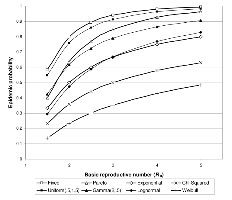
Figure 2: Probability of an epidemic in a homogeneous population as a function of $R_{0}$ for recovery time distributions from Table 1.

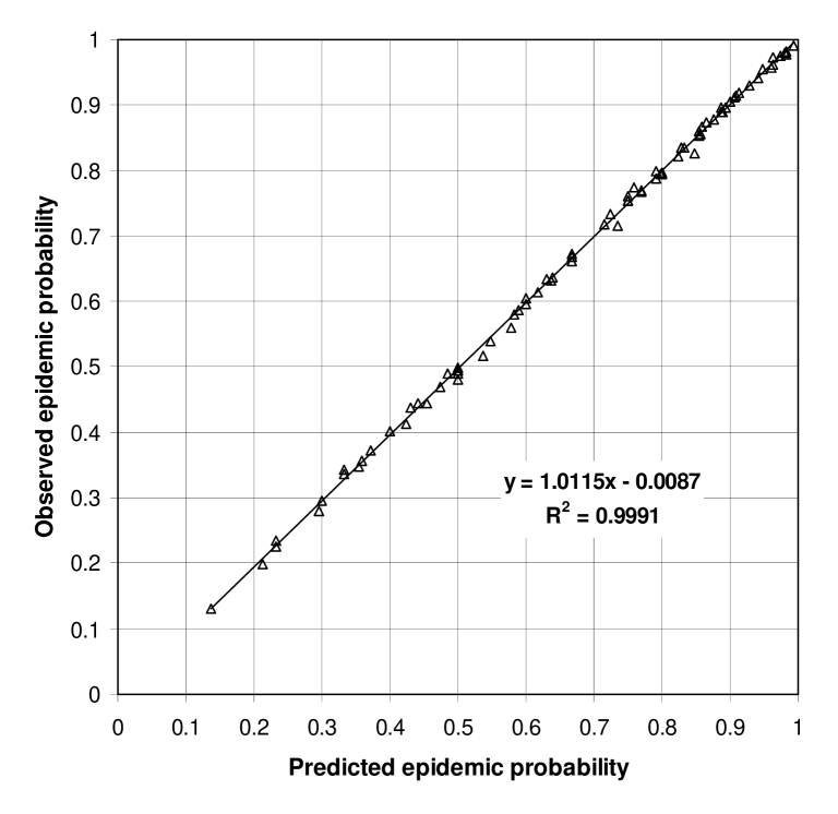
Figure 3: Scatterplot of observed and predicted epidemic probabilities for all homogeneous population models, with the linear regression equation and $R^{2}$.   

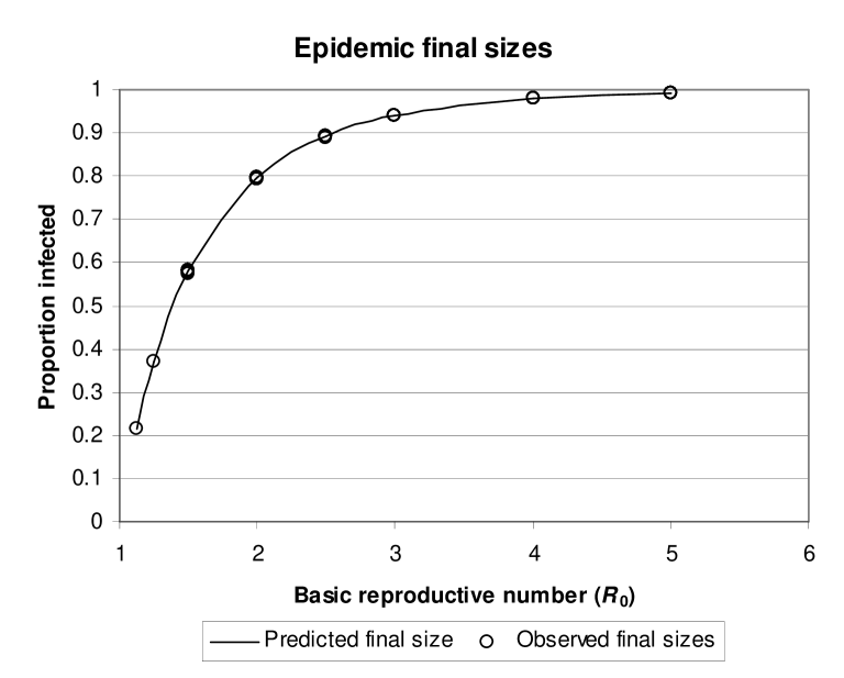
Figure 4: Predicted and observed final sizes of epidemics as a function of $R_{0}$ for all homogeneous population models.  The predicted final size was the same for all recovery time distributions.

In all homogeneous population models, an epidemic was said to occur when more than $10\%$ of the population was infected.  As outlined in Section 3, the predicted probability of an epidemic is $1-H^{out}(1)$ and the predicted final size of an epidemic is $1-H^{in}(1)$.  The predicted final size of an epidemic for a given $R_{0}$ was the same for all recovery time distributions, but Figure 2 shows that the probability of an epidemic depends on both $R_{0}$ and the recovery time distribution.  The probability and final size of an epidemic were equal only when the recovery time was fixed.  For all other recovery time distributions, the probability of an epidemic was less than its final size (this inequality is proven in [5]).  Figure 3 shows a good agreement between the predicted and observed probabilities of an epidemic and Figure 4 shows a good agreement between the observed and predicted final sizes of epidemics.

4.2 Heterogeneous populations

In the first two series of heterogeneous population models, the population consisted of two subpopulations $A$ and $B$ of equal size.  The average number of infectious contacts made by a member of subpopulation $B$ during his or her recovery period is $\lambda$.  We assumed the following infectious contact rates from $i$ to $j$ in a population of size $n$: $\frac{8}{3}\lambda(n-1)^{-1}$ when $i$ and $j$ are both members of subpopulation $A$, $\frac{4}{3}\lambda(n-1)^{-1}$ when $i$ and $j$ are members of different subpopulations, and $\frac{2}{3}\lambda(n-1)^{-1}$ when $i$ and $j$ are both in subpopulation $B$.  All models had a mean recovery time of one.  With these assumptions, the mean indegree and outdegree of subpopulation $A$ were $2\lambda$ and the mean indegree and outdegree of subpopulation $B$ were $\lambda$, producing a positive correlation between susceptibility and infectiousness.

When  the recovery period is fixed, the pgf for the degree distribution of the epidemic percolation network is

$$G(x,y)=.5e^{2\lambda(x-1)}e^{2\lambda(y-1)}+.5e^{\lambda(x-1)}e^{\lambda(y-1)}.$$

When the recovery period is exponentially distributed, the pgf for the degree distribution of the epidemic percolation network is

$$G(x,y)=.5\frac{e^{2\lambda(x-1)}}{1-2\lambda(y-1)}+.5\frac{e^{\lambda(x-1)}}{1-\lambda(y-1)}$$

Each model was run at $\lambda=.65,.7,.8,.9,1.0,1.1,1.2,1.3,$ and $1.4$.  At each $\lambda$, the model was run $10,000$ times.  For models with $\lambda>.65$, the population was $10,000$.  For $\lambda=.65$, the population size was $100,000$.  When $\lambda=.65$, epidemics occur even though the mean degree of the network is less than one.  Both series of models were implemented in Berkeley Madonna.

A third series of simulations was conducted in populations with various mixtures of recovery time distributions.  The population had $1,000$ individuals partitioned into subpopulations $A$ and $B$ of $500$ individuals each.  Each model was run under two scenarios: In the first scenario, subpopulation $A$ is twice as infectious per unit time and has the same mean recovery time as subpopulation $B$.  In the second scenario, both subpopulations are equally infectious per unit time but the mean recovery period of subpopulation $A$ is twice as long as that of $B$.  The degree distribution of the epidemic percolation network is identical under both scenarios.  In the first scenario, models were run for all nine possible combinations of the Fixed$(1)$, Uniform$(0,2)$, and Exponential$(1)$ recovery time distributions.  In the second scenario, models were run for all nine possible combinations of Fixed$(2)$, Uniform$(0,4)$, and Exponential$(.5)$ in subpopulation $A$ and Fixed$(1)$, Uniform$(0,2)$, and Exponential$(1)$ in subpopulation $B$.  These recovery time distributions are described in Table 1.  Every model was run $5,000$ times with $\lambda=2$.  An epidemic was defined as an outbreak that infected more than $15\%$ of the population.  A similar set of simulations was conducted where subpopulation $A$ had a mean indegree of $\lambda$ and a mean outdegree of $2\lambda$ while subpopulation $B$ had a mean indegree of $2\lambda$ and a mean outdegree of $\lambda$, producing a negative correlation between infectiousness and susceptibility.  All of these models were implemented in Mathematica.

In the first two series of heterogeneous models, an epidemic was defined to occur when more than $10\%$ of the population was infected.  The predicted probability and final size of an epidemic are $1-H^{out}(1)$ and $1-H^{in}(1)$, respectively, according to the epidemic percolation network.  According to a branching process approximation, the predicted probability of an epidemic is $1-h^{out}(1)$, where

$$h^{out}(z)=zG(1,h^{out}(z)),$$

and the predicted final size of an epidemic is $1-h^{in}(1)$, where

$$h^{in}(z)=zG(h^{in}(z),1).$$

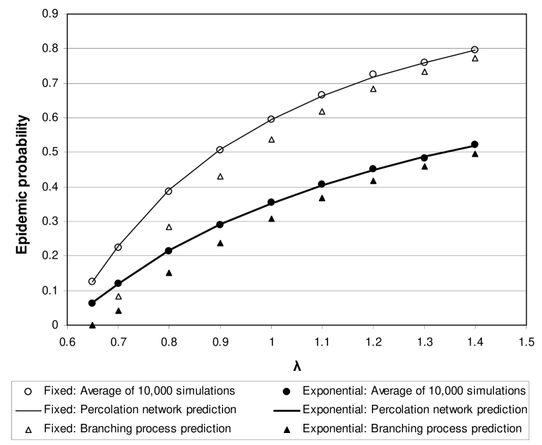
Figure 5: Predicted and observed probabilities of an epidemic as a function of $\lambda$ for the first two series of heterogeneous population models.  

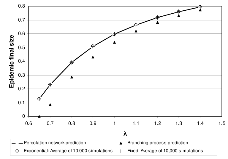
Figure 6: Predicted and observed final sizes of an epidemic as a function of $\lambda$ for the first two series of heterogeneous population models.  The final sizes of epidemics are the same for both fixed and exponentially-distributed recovery times.

Figures 5 and 6 compare the epidemic percolation network and branching process predictions of the probability and final size of an epidemic.  These models have a positive correlation between infectiousness and susceptibility, so persons infected through indigenous transmission are more infectious than persons randomly selected from the population.  Since the branching process approximation implicitly assumes that persons infected through indigenous transmission have the same outdegree distribution as the general population, it consistently underestimates both the probability and final size of an epidemic.  The epidemic percolation network consistently predicts the correct probability and final size of an epidemic.

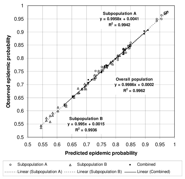
Figure 7: Scatterplot of observed and predicted epidemic probabilities in the third series of heterogeneous population models.  The ”subpopulation A” and ”subpopulation B” points show conditional epidemic probabilities given an initial case in subpopulation A and B respectively.  The ”combined” points show the epidemic probability when the initial case is randomly chosen from the entire population.  The linear regression equation and $R^{2}$ are shown separately for all three sets of points.

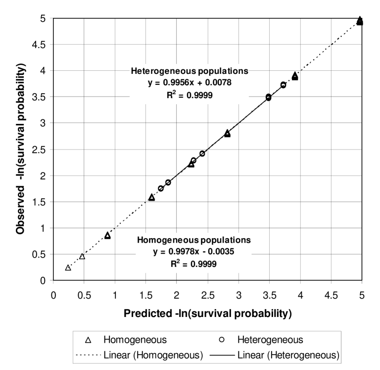
Figure 8: Scatterplot of the observed and predicted cumulative hazard of infection in an epidemic.  Linear regression equations and $R^{2}$ are shown separately for homogeneous and heterogeneous population models.

Figure 7 shows a scatterplot of observed and predicted epidemic probabilities for all heterogeneous population models.  The predicted probability of an epidemic for an initial case randomly chosen from the population is $1-H^{out}(1)$.  The “combined” points show the observed and predicted epidemic probabilities for an initial case randomly chosen from the overall population.  Let $G_{A}(x,y)$ and $G_{B}(x,y)$ be the pgf of the degree distributions of nodes in subpopulations $A$ and $B$ respectively.  The predicted probability of an epidemic for an initial case chosen randomly from subpopulation $A$ is $1-G_{A}(1,H_{f}^{out}(1))$, and the predicted probability of an epidemic for an initial case chosen randomly from subpopulation $B$ is $1-G_{B}(1,H_{f}^{out}(1))$.  The “subpopulation $A$” points show the observed and predicted epidemic probabilities for an initial case randomly chosen from subpopulation $A$, and the “subpopulation $B$” points show the observed and predicted epidemic probabilities for an initial case randomly chosen from subpopulation $B$.  All three sets of points are close to the diagonal, showing that epidemic percolation networks accurately predicted the probability of an epidemic.  The predicted cumulative hazard of infection in an epidemic is $-\ln(H^{in}(1))$.  Figure 8 shows a scatterplot of the observed and predicted cumulative hazard of infection in an epidemic for all heterogeneous population models.  All points are close to the diagonal, showing that epidemic percolation networks accurately predicted the final size of epidemics.

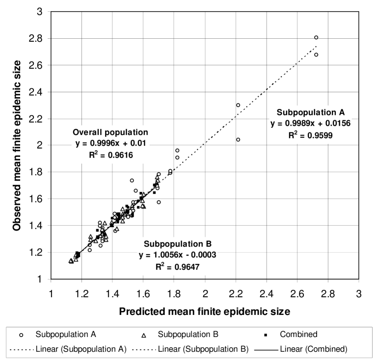
Figure 9: Scatterplot of observed and predicted mean sizes of outbreaks in the third series of heterogeneous population models.  Linear regression equations and $R^{2}$ are shown separately for an initial case randomly chosen from subpopulation $A$, subpopulation $B$, and from the overall population.

Figure 9 shows a scatterplot of the observed and predicted mean size of outbreaks in the third series of heterogeneous population models.  The mean size of an outbreak started by a single, randomly chosen imported infection is $H^{out\prime}(1)$.  The “combined” points show the observed and predicted mean outbreak size for an initial case randomly chosen from the overall population.  The mean size of an outbreak started by an imported infection randomly chosen from subpopulation $A$ is

$$\frac{\partial}{\partial z}G_{A}(1,H_{f}^{out}(z))|_{z=1,}$$

and the mean size of an outbreak started by an imported infection randomly chosen from subpopulation $B$ is

$$\frac{\partial}{\partial z}G_{B}(1,H_{f}^{out}(z))|_{z=1}.$$

The “subpopulation $A$” points show the observed and predicted mean outbreak size for an initial case randomly chosen from subpopulation $A$, and the “subpopulation $B$” points show the observed and predicted mean outbreak size for an initial case randomly chosen from subpopulation $B$.  All three sets of points are close to the diagonal, showing that epidemic percolation networks accurately predicted the mean sizes of finite epidemics in these models.  Models with higher epidemic probabilities tend to have smaller outbreak sizes because large outbreaks are more likely to “explode” and become epidemics.

5 Equivalence to classical epidemic theory

In this section, we show that epidemic percolation networks can reproduce much of the standard theory of epidemics.  When the indegree and outdegree are independent, the epidemic percolation networks predict the same distribution of outbreak sizes, epidemic threshold, and probability and final size of an epidemic as the forward and backward branching process approximations.  Epidemic percolation networks can also reproduce results from models developed specifically for special topics within infectious disease epidemiology.  Below, we give examples of the derivation of results from the epidemiology of sexually transmitted diseases, controlled diseases, and vector-borne diseases.

5.1 Branching processes

Much of the mathematical theory of epidemics has been derived using a branching process as an approximation to the initial spread of disease, where the “offspring” of an individual are the persons he or she infects [15, 7, 18].  The branching process approximation remains accurate until the first time at which an infectious individual transmits infection to a person who has already been infected, which happens after an arbitrarily long interval in the limit of a large population [15].  We will call this the ”forward” branching process approximation to the initial spread of disease, to distinguish it from the ”backward” branching process discussed later.

If the offspring distribution of a branching process has the pgf $g(x)$, then the probability that the branching process goes extinct is the smallest solution in $[0,1]$ of the equation $x=g(x)$.  If $h(z)$ is the pgf for the total number of individuals generated by the branching process (including the initial individual), then $h(z)=zg(h(z))$ [23].

Theorem 1

When an epidemic percolation network has independent indegree and outdegree, it predicts exactly the same outbreak size distribution, epidemic threshold, and probability of an epidemic (given the infection of a single randomly chosen node) as a forward branching process approximation to the initial spread of disease.

Proof. The pgf for the number of secondary infections produced by a randomly chosen imported infection is $G(1,y)$.  The number of secondary infections produced by persons infected through indigenous transmission has the pgf

$$G_{f}(1,y)=\frac{1}{\left\langle k_{d}\right\rangle}G^{(1,0)}(1,y)=G(1,y),$$

where the second equality follows from the independence of the indegree and outdegree.  Therefore, the initial spread of disease behaves like a branching process whose offspring distribution has the pgf $g_{f}(y)=G(1,y)$.  The probability of a self-limited outbreak (i.e. no epidemic) given the infection of a randomly chosen individual is the smallest solution in $[0,1]$ of $y=G(1,y)$, which is equivalent $y=g_{f}(y)$.  Similarly, $H_{f}^{out}(z)=H^{out}(z)$ and the pgf for outbreak sizes is $H^{out}(z)=zG(1,H^{out}(z))$, which is equivalent to $h(z)=zg_{f}(h(z))$.    

Another important application of branching processes to SIR models with random mixing is the use of a ”backward” branching process to predict the relative final size of an epidemic, in which the ”offspring” for each individual $i$ are the people who would make infectious contact with $i$ if they were infectious.  The relative final size of the epidemic is equal to the probability that the backward branching process never goes extinct [7].

Theorem 2

When an epidemic percolation network has independent indegree and outdegree, it predicts exactly the same relative final size of an epidemic as a backward branching process.

Proof. In the epidemic percolation network, the number of offspring in the backwards branching process for a randomly chosen individual has the pgf $G(x,1)$.  The pgf for the number of offspring of persons reached by going in reverse along a directed edge is

$$G_{r}(x,1)=\frac{1}{\left\langle k_{d}\right\rangle}G^{(0,1)}(x,1)=G(x,1),$$

where the final equality follows from the independence of the indegree and outdegree.  Therefore, the process of moving backwards along edges in the epidemic percolation network is a branching process whose offspring distribution has the pgf $g_{b}(x)=G(x,1)$.  The probability that a node is not infected in an epidemic is the smallest solution in $[0,1]$ of $x=G(x,1)$, which equivalent to $x=g_{b}(x)$.  Therefore, the epidemic percolation network and the branching process predict the same relative final size of an epidemic.     

In an SIR model whose epidemic percolation network has independent indegree and outdegree, the epidemic percolation network is a simultaneous mapping of the forward and backward branching processes.  However, a branching process assumes that the offspring distribution is the same in each generation of infection (because the same pgf $g(x)$ is used for each generation).  This assumption fails in an epidemic percolation network in which the indegree and outdegree are not independent.

Epidemic percolation networks generalize to models with arbitrary joint degree distributions because they allow the offspring distribution of the initial node to be different from the offspring distribution of all subsequent generations in the forward and backward branching processes.  If we go forward along edges starting from a randomly chosen node, the offspring distribution of the initial node has the pgf $G(1,y)$ and the offspring distribution of nodes in all subsequent generations has the pgf $G_{f}(1,y)$.  If we go backward starting from a randomly chosen node, then the offspring distribution of the initial node has the pgf $G(x,1)$ and all subsequent generations have the pgf $G_{r}(x,1)$.  When the indegree and outdegree are not independent, $G(1,y)\neq G_{f}(1,y)$ and $G(x,1)\neq G_{r}(x,1)$, so both branching process approximations break down.  We find it useful to think of the equations for the component size distributions in Section 3 as describing (forward or backward) branching processes in which the initial node is allowed to have a different offspring distribution from all subsequent generations.

By mapping the forward and backward infectious contact processes simultaneously, the crucial role of the GSCC in the emergence of epidemics becomes clear.  In a forthcoming manuscript, we analyze a proportionate mixing model with three subpopulations: One with the greatest probability of being in the GIN, one with the greatest probability of being in the GOUT, and one with the greatest probability of being in the GSCC.  Vaccinating nodes in the subpopulation most likely to be in the GSCC is shown to be the most efficient strategy for reducing both the probability and final size of an epidemic despite the fact that such nodes were of average infectiousness and susceptibility.  We have obtained similar results with network-based models.  Nodes with a high probability of being in the GSCC are the “core group” that sustains transmission of infection in the population.  If the forward and backward infectious contact processes are treated separately, the notion of the GSCC is lost.

5.2 Other results of epidemic theory

The use of probability generating functions on epidemic percolation networks allows many classical results from the theory of epidemics to be re-derived very easily.  Below, we give derivations of results from three different areas of infectious disease epidemiology.  The ability of epidemic percolation networks to encompass these results in a single conceptual framework is a striking demonstration of their utility and generality.

Example 1 (Sexually transmitted diseases)

For many sexually transmitted diseases, variation in levels of sexual activity affect the dynamics of disease transmission.  One important result is that $R_{0}$ for sexually transmitted diseases depends on both the mean and the variance of the number of sexual partners [18].  Let $I$ be a random variable representing the expected number of sexual partners a person has during his or her recovery period.  If the hazard of infection is proportional to $I$, then

$$R_{0}=\frac{T}{\mu_{I}}\left[\mu_{I}^{2}+\sigma_{I}^{2}\right],$$

where $\mu_{I}$ and $\sigma_{I}^{2}$ are the mean and variance of the number of sexual partners and $T$ is the probability of transmission for each partnership [18, 7].

We first partition the population into subpopulations $1,2,...$ such that subpopulation $i$ consists of all persons with $I=i$.  The proportion of the population in subpopulation $i$ is equal to $P(I=i)$.  Since there is a constant probability $T$ of transmission for each partnership and $I=i$ is the expected number of partners during the recovery period, the mean outdegree of subpopulation $i$ is $Ti$.  Since the hazard of infection in subpopulation $i$ is also proportional to $i$, the mean indegree of subpopulation $i$ must also be $Ti$.  The indegree and outdegree of each individual are conditionally independent given $I$, so the pgf for the degree distribution of nodes in subpopulation $i$ can be written

$$G_{i}(x,y)=G_{i}^{in}(x)G_{i}^{out}(y).$$

The pgf of the degree distribution of the epidemic percolation network is

$$G(x,y)=\sum_{i}P(I=i)G_{i}^{in}(x)G_{i}^{out}(y),$$

The overall mean degree is $T\mu_{I}$, and the epidemic threshold is

$$\frac{1}{T\mu_{I}}G^{(1,1)}(1,1)=\frac{T}{\mu_{I}}\sum_{i}i^{2}P(I=i)=\frac{T}{\mu_{I}}\left[\mu_{I}^{2}+\sigma_{I}^{2}\right].$$

Therefore, the epidemic percolation network correctly predicts the epidemic threshold for this model.  However, it can also predict the size distribution of outbreaks and the probability and final size of an epidemic.  Epidemic percolation networks can also be used to analyze SIR models with more complex relationships between sexual activity, infectiousness, and susceptibility.

Example 2 (Outbreaks of controlled diseases)

For diseases that have been eliminated within a specific country but are not eradicated worldwide (such as measles in the United States), imported cases and cases secondary to importation can still occur.  To evaluate the success of a disease elimination program, it is important to determine whether the observed pattern of outbreaks is consistent with sustained indigenous transmission.  This can be inferred from the final size distribution of outbreaks.  If infectiousness and susceptibility are independent and cases generate secondary cases according to a Poisson distribution with mean $R_{0}<1$, all epidemics are finite and epidemic sizes follow a Borel-Tanner distribution [24, 25].  The probability that an outbreak has a final size of $k$ is

$$\frac{R_{0}^{k-1}k^{k-2}e^{-R_{0}k}}{(k-1)!}.$$ (11)

The pgf for the Borel-Tanner distribution is the unique solution to the equation

$$h(z)=ze^{R_{0}(h(z)-1)}.$$ (12)

Below the phase transition, the pgf for the distribution of outbreak sizes in the epidemic percolation network is $H^{out}(z)$.  Since the incoming and outgoing degree are independent and the outgoing degree is Poisson distributed with mean $R_{0}$,

$$G_{f}(1,y)=G(1,y)=e^{R_{0}(y-1)}$$

But then

$$H_{f}^{out}(z)=H^{out}(z)=ze^{R_{0}(H^{out}(z)-1)},$$ (13)

which is identical to equation (12).  Therefore, $H^{out}(z)=h(z)$, so the out-component sizes in the epidemic percolation network have a Borel-Tanner distribution.  Using the fact that the probability of having an outbreak of size one is $e^{-R_{0}}$, it is easy to check that the first few iterations of equation (13) produce coefficients of the form in equation (11).

Example 3 (Vector-borne diseases)

The model of malaria developed by Ross and Macdonald consists of humans and mosquitoes.  Infected humans recover from malaria at a constant rate $\gamma$, so the average recovery period is $\gamma^{-1}$.  There are $m$ susceptible mosquitoes that bite with a rate $a$ and are infected with probability $c$ when they bite an infectious human, so each infectious human infects an average of $(amc)\gamma^{-1}$ susceptible mosquitoes.  The mortality rate of mosquitoes is $\mu$, so they survive for an average of $\mu^{-1}$ time units after being infected.  When an infectious mosquito bites a susceptible human, the human is infected with probability $b$, so each infectious mosquito infects an average of $(ab)\mu^{-1}$ humans.  The epidemic threshold in this model is defined by

$$R_{0}=\frac{ma^{2}bc}{\mu\gamma}.$$

This was one of the earliest applications of the basic reproductive number [18].

The full epidemic percolation network for a vector-borne disease would include nodes representing humans and vectors.  Humans infect vectors and vectors infect humans, so every edge in this epidemic percolation network links nodes of different types.  Such a network is called a bipartite network.  Probability generating functions can be used to analyze undirected bipartite networks [2], and these methods can be adapted to directed bipartite graphs.  Using the subscript $h$ for host and $v$ for vector, let $G_{h}(x,y)$ be the pgf for the degree distribution among humans and let $G_{v}(x,y)$ be the pgf for the degree distribution among vectors.  The epidemic percolation network among humans can then be constructed by drawing an edge from person $i$ to person $j$ if there is a vector that transfers infection from $i$ to $j$.  The pgf for the degree distribution in the human-human epidemic percolation network is

$$G_{H}(x,y)=\sum_{j=0}^{\infty}\sum_{k=0}^{\infty}p_{jk}^{h}(G_{vr}(x,1))^{j}(G_{vf}(1,y))^{k}=G_{h}(G_{vr}(x,1),G_{vf}(1,y)),$$

where $p_{jk}^{h}$ is the probability that a human node in the human-vector epidemic percolation network has $j$ incoming edges and $k$ outgoing edges, $G_{vr}(x,y)$ is the pgf for the degree of a vector reached by going backwards along an edge, and $G_{vf}(x,y)$ is the pgf for the degree of a vector reached by going forward along an edge.  The outbreak size distribution, the epidemic threshold, and the probability and final size of an epidemic among humans can be predicted using $G_{H}(x,y)$.

In the Ross-Macdonald model, infectiousness and susceptibility are independent among both humans and mosquitoes.  Therefore, $G_{hf}(1,y)=G_{h}(1,y)$ and $G_{vf}(1,y)=G_{v}(1,y)$.  The pgf for the out-degree of human nodes is

$$G_{h}(1,y)=\int_{0}^{\infty}e^{(amc)t(y-1)}\gamma e^{-\gamma t}dt=\frac{1}{1-amc\gamma^{-1}(y-1)},$$

and the pgf for the out-degree of mosquito nodes is

$$G_{v}(1,y)=\int_{0}^{\infty}e^{(ab)t(y-1)}\mu e^{-\mu t}dt=\frac{1}{1-ab\mu^{-1}(y-1)}.$$

Since the indegree and outdegree are independent in the human-to-human epidemic percolation network,

$$G_{Hf}(1,y)=G_{H}(1,y)=G_{h}(1,G_{vf}(1,y)).$$

Taking the derivative of $G_{Hf}(1,y)$ at $y=1$,

$$G_{Hf}^{(0,1)}(1,1)=G_{h}^{(0,1)}(1,1)G_{vf}^{(0,1)}(1,1)=\frac{amc}{\gamma}\cdot\frac{ab}{\mu},$$

and we see that the epidemic threshold occurs when $\frac{ma^{2}bc}{\mu\gamma}=1$, which is identical to the threshold derived by Ross and Macdonald.

6 Discussion

For the epidemic models considered in this paper, methods of finding the exact distribution of outbreak sizes for a homogeneous population of any fixed size $n$ exist [15, 7, 17].  However, these methods involve solving a recursive system of $n$ equations.  By performing these calculations in the limit of a large population, the methods presented in this paper allow a much simpler derivation of the distribution of self-limited outbreak sizes, the epidemic threshold, and the probability and final size of an epidemic.  Our methods also generalize much more easily to heterogeneous populations.

As proven in the Appendix, the problem of analyzing the final outcomes of any time-homogeneous stochastic SIR model can be reduced to the problem of analyzing the components of an epidemic percolation network.  In [5], we showed how epidemic percolation networks can be used to analyze network-based models of the type studied by Newman [1].  In this paper, we showed that epidemic percolation networks can be used to analyze stochastic SIR models with random and proportionate mixing.  In the limit of a large population, the epidemic percolation network for these models is purely directed.  Using the probability generating function for its degree distribution, we accurately predicted the mean size of outbreaks and the probability and final size of epidemics for a variety of models in homogeneous and heterogeneous populations.

The ability of epidemic percolation networks to analyze both network-based and fully-mixed epidemic models makes them a simple but powerful generalization of earlier methods of analyzing stochastic SIR models.  We showed that epidemic percolation networks with independent indegree and outdegree are equivalent to forward and backward branching processes, and we used epidemic percolation networks to re-derive classical results from sexually transmitted diseases, vector-borne diseases, and controlled diseases.  Epidemic percolation networks may also provide a novel and useful qualitative insight into the control of epidemics.  The emergence of epidemics corresponds to the emergence of the GSCC in the epidemic percolation network, so nodes with a high probability of being in the GSCC may be important targets for interventions designed to reduce the probability and final size of an epidemic.

Acknowledgements: This work was supported by the US National Institutes of Health cooperative agreement 5U01GM076497 ”Models of Infectious Disease Agent Study” (E.K.) and Ruth L. Kirchstein National Research Service Award 5T32AI007535 ”Epidemiology of Infectious Diseases and Biodefense” (E.K.), as well as a research grant from the Institute for Quantitative Social Sciences at Harvard University (E.K.).  We are grateful for the comments of Marc Lipsitch, James Maguire, Jacco Wallinga, Joel C. Miller, and the anonymous referees of JTB.  E.K. would also like to thank Charles Larson and Stephen P. Luby of the Health Systems and Infectious Diseases Division of ICDDR,B (Dhaka, Bangladesh).

Appendix A Epidemic percolation networks

It is possible to define epidemic percolation networks for a much wider range of stochastic epidemic models than that from the Introduction.  First, we specify an SIR epidemic model using probability distributions for infectious periods in individuals and times from infection to infectious contact in ordered pairs of individuals.  Second, we outline time-homogeneity assumptions under which the epidemic percolation network is defined.  Finally, we define infection networks and use them to show that the final outcome of the epidemic model depends only on the set of initial infections and the epidemic percolation network.  This discussion is adapted from that of our previous paper [5].

A.1 Model specification

Suppose there is a closed population in which every susceptible person is assigned an index $i\in\{1,...,n\}$.  A susceptible person is infected upon infectious contact, and infection leads to recovery with immunity or death.  Each person $i$ is infected at his or her infection time $t_{i}$, with $t_{i}=\infty$ if $i$ is never infected.  Person $i$ is removed (i.e. recovers from infectiousness or dies) at time $t_{i}+r_{i}$, where the recovery period $r_{i}$ is a random variable with the cumulative distribution function (cdf) $F_{i}(r)$.  The recovery period $r_{i}$ may be the sum of a latent period, when $i$ is infected but not yet infectious, and an infectious period, when $i$ can transmit infection.  We assume that all infected persons have a finite recovery period.  Let $S(t)=\{i:t_{i}>t\}$ be the set of susceptible individuals at time $t$.  Let $t_{(1)}\leq t_{(2)}\leq...\leq t_{(n)}$ be the order statistics of $t_{1},...,t_{n}$, and let $i_{k}$ be the index of the $k^{\text{th}}$ person infected.

When person $i$ is infected, he or she makes infectious contact with person $j\neq i$ after an infectious contact interval $\tau_{ij}$.  Given $r_{i}$, each $\tau_{ij}$ has a conditional cdf $F_{ij}(\tau|r_{i})$.  Let $\tau_{ij}=\infty$ if person $i$ never makes infectious contact with person $j$, so $F_{ij}(\tau|r_{i})$ may have a probability mass concentrated at infinity.  Person $i$ cannot transmit disease before being infected or after recovering from infectiousness, so $F_{ij}(\tau|r_{i})=0$ for all $\tau\leq 0$ and $F_{ij}(\tau|r_{i})$ is equal to the conditional probability of transmission from $i$ to $j$ given $r_{i}$ for all $\tau\in[r_{i},\infty)$.   The infectious contact time $t_{ij}=t_{i}+\tau_{ij}$ is the time at which person $i$ makes infectious contact with person $j$.  If person $j$ is susceptible at time $t_{ij}$, then $i$ infects $j$ and $t_{j}=t_{ij}$.  If $t_{ij}<\infty$, then we must have $t_{j}\leq t_{ij}$ because person $j$ avoids infection at $t_{ij}$ only if he or she has already been infected.

For each person $i$, let his or her importation time $t_{0i}$ be the first time at which he or she experiences infectious contact from outside the population, with $t_{0i}=\infty$ if this never occurs.  Let $F_{0}(\mathbf{t}_{0})$ be the cdf of the importation time vector $\mathbf{t}_{0}=(t_{01},t_{02},...,t_{0n})$.

A.2 Epidemic algorithm

Before an epidemic begins, an importation time vector $\mathbf{t}_{0}$ is chosen.  The epidemic begins with the introduction of infection at time $t_{(1)}=\min_{i}(t_{0i})$.  Person $i_{1}$ is assigned an recovery period $r_{i_{1}}$.  Every person $j\in S(t_{(1)})$ is assigned an infectious contact time $t_{i_{1}j}=t_{(1)}+\tau_{i_{1}j}$.  We assume that there are no tied infectious contact times less than infinity.  The second infection occurs at $t_{(2)}=\min_{j\in S(t_{(1)})}\min(t_{0j},t_{i_{1}j})$, which is the time of the first infectious contact after person $i_{1}$ is infected.  Person $i_{2}$ is assigned an recovery period $r_{i_{2}}$.  After the second infection, each of the remaining susceptibles is assigned an infectious contact time $t_{i_{2}j}=t_{(2)}+\tau_{i_{2}j}$.  The third infection occurs at $t_{(3)}=\min_{j\in S(t_{(2)})}\min(t_{0j},t_{i_{1}j},t_{i_{2}j})$, and so on.  After $k$ infections, the next infection occurs at $t_{(k+1)}=\min_{j\in S(t_{(k)})}\min(t_{0j},t_{i_{1}j},...,t_{i_{k}j})$.  The epidemic stops after $m$ infections if and only if $t_{(m+1)}=\infty$.

A.3 Time homogeneity assumptions

In principle, the above epidemic algorithm could allow the distributions of the recovery period and outgoing infectious contact intervals for individual $i$ to depend on all information about the epidemic available up to time $t_{i}$.  In order to generate an epidemic percolation network, we must ensure that the joint distribution of recovery periods and conditional transmission probabilities for all ordered pairs of individuals are defined a priori.  In order to do this, we place the following restrictions on the model:

1. We assume that the distribution of the recovery period vector $\mathbf{r}=(r_{1},r_{2},...,r_{n})$ does not depend on the importation time vector $\mathbf{t}_{0}$, the contact interval matrix $\mathbf{\tau}=[\tau_{ij}]$, or the history of the epidemic.

2. We assume that the distribution of the infectious contact interval matrix $\mathbf{\tau}$ does not depend on $\mathbf{t}_{0}$ or on the history of the epidemic.

With these time-homogeneity assumptions, the cumulative distribution functions $F(\mathbf{r})$ of recovery periods and $F(\mathbf{\tau}|\mathbf{r})$ of infectious contact intervals are defined a priori.  Given$\ \mathbf{r}$ and $\mathbf{\tau}$, the epidemic percolation network is a semi-directed network in which there is a directed edge from $i$ to $j$ iff $\tau_{ij}<\infty$ and $\tau_{ji}=\infty$, a directed edge from $j$ to $i$ iff $\tau_{ij}=\infty$ and $\tau_{ji}<\infty$, and an undirected edge between $i$ and $j$ iff $\tau_{ij}<\infty$ and $\tau_{ji}<\infty$.  The entire time course of the epidemic is determined by $\mathbf{r}$, $\mathbf{\tau}$, and $\mathbf{t}_{0}$.  However, its final size depends only on the set $\{i:t_{0i}<\infty\}$ of imported infections and the epidemic percolation network.  In order to prove this, we first define the infection network, which records the chain of infection from a single realization of the epidemic model.

A.4 Infection networks

Let $v_{i}$ be the index of the person who infected person $i$, with $v_{i}=0$ for imported infections and $v_{i}=\infty$ for uninfected nodes.  If tied finite infectious contact times have probability zero, then $v_{i}$ is the unique $j$ such that $t_{ji}=t_{i}$.  If tied finite infectious contact times are possible, then choose $v_{i}$ from all $j$ such that $t_{ji}=t_{i}$.  The infection network is a network with an edge set $\{v_{i}i:0<v_{i}<\infty\}$.  It is a subgraph of the epidemic percolation network because $\tau_{v_{i}i}<\infty$ for every edge $v_{i}i$.  Since each node has at most one incoming edge, all components of the infection network are trees.  Every imported case is either the root node of a tree or an isolated node.

The infection network can be represented by a vector $\mathbf{v}=(v_{1},..,v_{n})$, which is identical to the ”infection network” defined by Wallinga and Teunis [26].  If $v_{j}=0$, then its infection time is specified by $\mathbf{t}_{0}$.  If $j$ was infected through transmission within the population, then it is connected to an imported infection $imp_{j}$ in the infection network and its infection time is

$$t_{j}=t_{imp_{j}}+\sum_{k=1}^{m}\tau_{e_{k}^{\ast}},$$

where the edges $e_{1}^{\ast},...,e_{m}^{\ast}$ form a directed path from $imp_{j}$ to $j$.  This path is unique because all nontrivial components of the infection network are trees.  The infection times of all other nodes are infinite.  The removal time of each node $i$ is $t_{i}+r_{i}$.  Therefore, the entire time course of the epidemic is determined by the importation time vector $\mathbf{t}_{0}$, the recovery period vector $\mathbf{r}$, the infectious contact interval matrix $\mathbf{\tau}$.

A.5 Final outcomes and percolation networks

Theorem 3

In an epidemic with recovery period vector $\mathbf{r}$ and infectious contact interval matrix $\mathbf{\tau}$, a node is infected if and only if it is in the out-component of a node $i$ with $t_{0i}<\infty$ in the epidemic percolation network.  Equivalently, a node is infected if and only if its in-component includes a node $i$ with $t_{0i}<\infty$.

Proof. Suppose that person $j$ is in the out-component of a node $i$ with $t_{0i}<\infty$ in the epidemic percolation network.  Then there is a series of edges $e_{1},...e_{m}$ such that the initial node of $e_{1}$ is $i$, the terminal node of $e_{m}$ is $j$, and $\tau_{e_{k}}<\infty$ for all $1\leq k\leq m$.  Person $j$ receives an infectious contact at or before

$$t_{j}^{\ast}=t_{0i}+\sum_{k=1}^{m}\tau_{e_{k}}<\infty,$$

so $t_{j}\leq t_{j}^{\ast}<\infty$ and $j$ must be infected during the epidemic.  To prove the converse, suppose that $t_{j}<\infty$.  Then there exists an imported case $i$ and a directed path with edges $e_{1},...,e_{m}$ from $i$ to $j$ such that

$$t_{j}=t_{i}+\sum_{k=1}^{m}\tau_{e_{k}}.$$

Since $t_{j}<\infty$, it follows that all $\tau_{e_{k}}<\infty$.  But then each $e_{k}$ must be an edge with the proper direction in the epidemic percolation network, so $j$ is in the out-component of $i$.      

By the law of iterated expectation (conditioning on $\mathbf{\tau})$, this result implies that the probability distribution of outbreak sizes caused by the introduction of infection to node $i$ is identical to that of his or her out-component sizes in the probability space of epidemic percolation networks.  Furthermore, the probability that person $i$ gets infected in an epidemic is equal to the probability that his or her in-component contains at least one imported infection.  In the limit of a large population, the probability that node $i$ is infected in an epidemic is equal to the probability that he or she is in the GOUT and the probability that an epidemic results from the infection of node $i$ is equal to the probability that he or she is in the GIN.

Appendix B Tables and figures

Distribution	Density function	Support	Variance	P($t\leq.5$)
Uniform$(.5,1.5)$	$1$	$.5\leq t\leq 1.5$	$.0833$	$0$
$.4+$Gamma$(3,.2)$	$62.5(t-.4)^{2}e^{-5(t-.4)}$	$.4\leq t<\infty$	$.12$	$.0143877$
$.5+$Exponential$(2)$	$2e^{-2(t-.5)}$	$.5\leq t<\infty$	$.25$	$0$
Uniform$(0,2)$	$.5$	$0\leq t\leq 2$	$.333$	$.25$
Gamma$(2,.5)$	$4te^{-2t}$	$0\leq t<\infty$	$.5$	$.264241$
Exponential$(1)$	$e^{-t}$	$0\leq t<\infty$	$1$	$.393469$
LogNormal$(-.5,1)$	$\frac{1}{t\sqrt{2\pi}}e^{-.5(.5+\ln t)^{2}}$	$0\leq t<\infty$	$1.71828$	$.423422$
ChiSquare$(1)$	$\frac{1}{\sqrt{2\pi t}}e^{-.5t}$	$0\leq t<\infty$	$2$	$.5205$
Weibull$(.5,.5)$	$\frac{1}{\sqrt{2t}}e^{-\sqrt{2t}}$	$0\leq t<\infty$	$5$	$.632121$
Pareto$(.5$,$2)$	$.5t^{-3}$	$.5\leq t<\infty$	$\infty$	$0$
Uniform$(0,4)$*	$.25$	$0\leq t\leq 4$
Exponential$(.5)$*	$.5e^{-.5t}$	$0\leq t<\infty$

Table 1: Recovery time distributions for the third series of homogeneous population models. From top to bottom, they are in order of increasing variance. The bottom two distributions are used only in the third series of heterogeneous population models.

References

- [1] M. E. J. Newman (2002). Spread of epidemic disease on networks. Physical Review E 66, 016128.
- [2] M. E. J. Newman, S. H. Strogatz, and D. J. Watts (2001). Random graphs with arbitrary degree distributions and their applications, Physical Review E 64: 026118.
- [3] M. Boguñá and M. A. Serrano (2005). Generalized percolation in random directed networks. Physical Review E 72: 016106.
- [4] L. A. Meyers, M. E. J. Newman, and B. Pourbohloul (2006). Predicting epidemics on directed contact networks. Journal of Theoretical Biology 240(3): 400-418.
- [5] E. Kenah and J. M. Robins (2007). Second look at the spread of epidemics on networks. To be published in Physical Review E 76(3); also available at arXiv.org: q-bio.QM/0610057.
- [6] K. Kuulasmaa (1982). The spatial general epidemic and locally dependent random graphs. Journal of Applied Probability 19(4): 745-758 (1982).
- [7] O. Diekmann and J. A. P. Heesterbeek (2000). Mathematical Epidemiology of Infectious Diseases: Model Building, Analysis and Interpretation. Chichester, UK: John Wiley & Sons.
- [8] A. Broder, R. Kumar, F. Maghoul, P. Raghavan, S. Rajagopalan, R. Stata, A. Tomkins, and J. Weiner (2000). Graph structure in the Web. Computer Networks 33: 309-320.
- [9] S.N. Dorogovtsev, J.F.F. Mendes, and A.N. Sakhunin (2001). Giant strongly connected component of directed networks. Physical Review E 64: 025101(R).
- [10] R. Albert and A.-L. Barabási (2002). Statistical mechanics of complex networks. Reviews of Modern Physics 74: 47-97.
- [11] M. E. J. Newman (2003a). The structure and function of complex networks. SIAM Reviews 45(2): 167-256.
- [12] M. E. J. Newman (2003b). Random graphs as models of networks, in Handbook of Graphs and Networks, pp. 35-68. S. Bornholdt and H. G. Schuster, eds. Berlin: Wiley-VCH.
- [13] M.E.J. Newman, A.-L. Barabási, and D.J. Watts (2006). The Structure and Dynamics of Networks (Princeton Studies in Complexity). Princeton: Princeton University Press.
- [14] N. Schwartz, R. Cohen, D. ben-Avraham, A.-L. Barabási, and S. Havlin (2002). Percolation in directed scale-free networks. Physical Review E 66: 015104(R).
- [15] H. Andersson and T. Britton (2000). Stochastic Epidemic Models and Their Statistical Analysis (Lecture Notes in Statistics v.151). New York: Springer-Verlag.
- [16] L. M. Sander, C. P. Warren, I. M. Sokolov, C. Simon, and J. Koopman (2002). Percolation on heterogeneous networks as a model for epidemics. Mathematical Biosciences 180: 293-305.
- [17] D. J. Daley & J. Gani (1999). Epidemic Modelling: An Introduction (Cambridge Studies in Mathematical Biology). Cambridge, UK: Cambridge University Press.
- [18] R. M. Anderson and R. M. May (1991). Infectious Diseases of Humans: Dynamics and Control. New York: Oxford University Press.
- [19] D.J. Watts and S. Strogatz (1998). Collective dynamics of ’small-world’ networks. Nature 393: 440-442.
- [20] F. Ball and P. Neal (2002). A general model for stochastic SIR epidemic models with two levels of mixing. Mathematical Biosciences 180: 73-102.
- [21] M. Keeling (2005). The implications of network structure for epidemic dynamics. Theoretical Population Biology 67: 1-8.
- [22] M.A. Serrano and M. Boguñá (2006). Percolation and epidemic thresholds in clustered networks. Physical Review Letters 97: 088701.
- [23] A. Gut (1995). An Intermediate Course in Probability. New York: Springer-Verlag.
- [24] G. De Serres, N. J. Gay, and C. P. Farrington (2000). Epidemiology of transmissible diseases after elimination. American Journal of Epidemiology 151(11): 1039-1048.
- [25] F. A. Haight, M. A. Breuer (1960). The Borel-Tanner distribution. Biometrika 47(1,2): 143-146.
- [26] J. Wallinga and P. Teunis (2004). Different epidemic curves for Severe Acute Respiratory Syndrome Reveal Similar Impacts of Control Measures. American Journal of Epidemiology 160(6): 509-516.