Oscillations in two-species models: tying the stochastic and deterministic approaches

Abstract

We analyze general two-species stochastic models, of the kind generally used for the study of population dynamics. We show that the conditions for the stochastic (microscopic) model to display approximate sustained oscillatory behavior are governed by the parameters of the corresponding deterministic (macroscopic) model. We provide a quantitative criterion for the quality of the stochastic oscillation, using a dimensionless parameter that depends only on the deterministic model. When this parameter is small, the oscillations are clear, and the frequencies of the stochastic and deterministic oscillations are close, for all stochastic models compatible with the same deterministic one. On the other hand, when it is large, the oscillations cannot be distinguished from a noise.

It is well known that the dynamics of many systems of two species can display an oscillatory behavior in the populations of both agents. This happens in predator-prey systems begon , in models of measles epidemics wilson45 , in chemical systems such as those exemplified by the Brusselator prigogine68 , etc. These systems are usually modelled by a set of two coupled ordinary differential equations, which are assumed to represent a macroscopic level of description of the system. Oscillations can appear in these models as limit-cycle solutions to the equations. However, it frequently happens that the macroscopic model only has damped oscillatory solutions, even though the modelled system displays sustained oscillations in its populations in the same region of parameter values. Examples of this are not uncommon in population dynamics (see, e.g., the discussion in renshaw with regard to predator-prey and measles problems). It has often been noted that the stochastic counterpart of these models—assumed to represent a more microscopic level description of the same system— usually do display a kind of sustained oscillatory behavior, with a frequency very similar to the one of the damped solutions of the differential equations bartlett57 ; hethcote89 ; solari01 (see Fig. 1 for an example based on a susceptible-infected epidemic model). These oscillations are said to be generated by the demographic, or intrinsic, noise mckane05 . The problem is that stochasticity precludes a clear-cut definition of “oscillations” for such systems. Therefore, the comparison between the results of the stochastic and deterministic approaches is often made on a qualitative basis.

In this Letter we address the problem of sustained oscillations in stochastic models, in an attempt to characterize the oscillatory regime. We show that the conditions for well defined oscillations are given by the parameters of the corresponding macroscopic (deterministic) model only, disregarding the details of the microscopic (stochastic) one. In other words, this general result proves that the conditions are the same for any stochastic model that corresponds to the same macroscopic one. To this end, we define a criterion of “quality” of oscillatory behavior for a large class of stochastic two-species systems and we show, by means of a van Kampen expansion of the master equation, that the information given by the deterministic system—embodied in a deterministic parameter—is enough to provide good bounds on this quality. In other words, we show that the quality of the oscillations is only weakly dependent on the details of the demographic noise. Moreover, it is shown that oscillations become clear if and only if the deterministic parameter vanishes. We also suggest a heuristic value for the quality below which one can be almost certain that the evolution of both populations does “look” oscillatory.

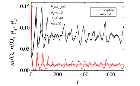
Figure 1: Deterministic dynamics (smooth lines) and one stochastic realization (fluctuating lines) of an SI epidemic model (susceptible and infected, respectively A and B). The dynamics includes birth and death processes in both populations, and contagion. A self-limiting intraspecific competition mechanism is implemented as in mckane04 ; mckane05 , with a total system size $\Omega=5\!\times\!10^{5}$. Transition rates are: $T_{10}=2(b_{A}\phi_{A}+b_{B\!A}\,\phi_{B})(1-\phi_{A}-\phi_{B})$, $T_{-10}=d_{A}\phi_{A}$, $T_{0-1}=d_{B}\phi_{B}$, $T_{-11}=2p\phi_{A}\phi_{B}$ (see Eq. (1)).

We consider systems of two populations, A and B, described by stochastic variables $m(t)$ and $n(t)$. The state of the system is defined by the joint probability $P(m,n;t)$ that the system has $m$ individuals of species A, and $n$ individuals of species B. The transition from a state with $(m,n)$ individuals to a state with $(m+i,n+j)$ individuals takes place at a rate:

$$T(m+i,n+j|m,n)=f(\Omega)T_{ij}(\frac{m}{\Omega},\frac{n}{\Omega}),$$ (1)

where $-k<i<k$ and $-k<j<k$. $\Omega$ is a scale parameter that governs the fluctuations of the stochastic evolution. Its precise definition depends on the system, but one chooses it in such a way that for large $\Omega$ the fluctuations are small. It usually represents the volume containing the reactants in chemical systems vankampen , or the available resources in biological ones mckane05 . The constant $k$ gives the maximal number of elements that can appear, or disappear, from a given population at each step of the dynamics. The most common choice are one-step processes, with $k=1$.

The evolution of the probability $P(m,n;t)$ is given by the master equation vankampen :

$$\frac{\partial P(m,n;t)}{\partial t} = \sum_{ij}P(m-i,n-j;t)\,T_{ij}(\frac{m-i}{\Omega},\frac{n-j}{\Omega})$$ (2)

$$-P(m,n;t)\sum_{ij}T_{ij}(\frac{m}{\Omega},\frac{n}{\Omega}),$$

where, as in the rest of this Letter, the summation indices run from $-k$ to $k$.

Except for a few simple cases, this equation is extremely difficult to solve exactly. For this reason many methods have been devised to look for approximate solutions. Perhaps the best known, and most applied, is the van Kampen expansion vankampen . In the following we sketch the main steps leading to the series solution (a detailed account can be found in van Kampen’s book vankampen ).

If one assumes that, at time zero, the system is in a state where both populations have well defined macroscopical values, $P(m,n)=\delta(m-m_{0})\delta(n-n_{0})$, with the initial values of order $O(\Omega)$, it is reasonable to expect that at later times $P(m,n)$ will have a sharp peak at some position of order $O(\Omega)$ (in both populations), and a width of order $O(\Omega^{1/2})$. That is, the fluctuating populations will satisfy $m=\Omega\phi_{A}+\sqrt{\Omega}\xi_{A}$ and $n=\Omega\phi_{B}+\sqrt{\Omega}\xi_{B}$, where the variables $\phi$ represent the “macroscopic” evolution, while the stochastic variables $\xi$ represent fluctuations around them. Replacing this in Eq. (2), equating terms of the same order in $\Omega$ and adequately rescaling the time, one obtains, for the leading order:

$$\dot{\phi}_{A} = \sum_{ij}i\,T_{ij}(\phi_{A},\phi_{B})\equiv C_{A}(\phi_{A},\phi_{B}),$$

$$\dot{\phi}_{B} = \sum_{ij}j\,T_{ij}(\phi_{A},\phi_{B})\equiv C_{B}(\phi_{A},\phi_{B}).$$ (3)

These equations, called deterministic or macroscopic, are usually the starting point of many models of chemical and biological systems. They are generally written down from macroscopic considerations of the population dynamics, disregarding its individual level origin. To analyze the differences between the stochastic (individual level) and the deterministic (population level) approaches one usually chooses a stochastic model that gives the right deterministic equations. In the limit of infinite size ($\Omega\to\infty$), Eqs. (2) are also satisfied by the average populations.

The deterministic equilibria are obtained by solving the system $C_{A}(\phi_{A},\phi_{B})=C_{B}(\phi_{A},\phi_{B})=0$, and their stability is studied by means of a linear stability analysis. When the system is close to a stable equilibrium, its evolution can be approximated by that of a damped oscillator. In the underdamped regime, the damping factor and the frequency of oscillation are, respectively:

$$\gamma = \Delta\epsilon/2,$$

$$\omega_{d}^{2} = \Delta(1-\epsilon^{2}/4),$$ (4)

with

$$\epsilon=|T|/\sqrt{\Delta},$$ (5)

where $\Delta$ is the Jacobian of $\vec{C}$, and $T$ its trace:

$$\Delta = C_{A,A}C_{B,B}-C_{A,B}C_{B,A},$$

$$T = C_{A,A}+C_{B,B},$$ (6)

where $C_{i,j}=\frac{\partial C_{i}}{\partial\phi_{j}}$. The underdamped regime is therefore given by the condition $\epsilon<2$. We show below that this parameter, which depends only on the parameters of the macroscopic Eq. (3), plays a fundamental role in the characterization of the oscillations of stochastic origin. Notice also that the number of oscillations observed in the characteristic time $\gamma^{-1}$ depends only on $\epsilon$ (for small $\epsilon$, it is just $2/\epsilon$).

The following order in the van Kampen expansion gives the evolution of $\Pi(\xi_{A},\xi_{B},t)$, the joint probability function of the fluctuations, in the form of a Fokker-Planck equation. To look for oscillations in the fluctuations it is easier to work with the equivalent Langevin equations, as shown by McKane mckane05 :

$$\dot{\xi}_{A} = -C_{A,A}\xi_{A}-C_{A,B}\xi_{B}+L_{A}(t)$$

$$\dot{\xi}_{B} = -C_{B,A}\xi_{A}-C_{B,B}\xi_{B}+L_{B}(t)$$ (7)

where $L_{A}(t)$ and $L_{B}(t)$ are delta-correlated Gaussian noises of zero mean, satisfying $\langle L_{A}(t)L_{A}(t^{\prime})\rangle=D_{A}\delta(t-t^{\prime})$, $\langle L_{B}(t)L_{B}(t^{\prime})\rangle=D_{B}\delta(t-t^{\prime})$, and $\langle L_{A}(t)L_{B}(t^{\prime})\rangle=D_{AB}\delta(t-t^{\prime})$. The noise intensities are given by:

$$D_{A}(\phi_{A},\phi_{B}) = \sum_{i,j}i^{2}\,T_{ij}(\phi_{A},\phi_{B}),$$

$$D_{B}(\phi_{A},\phi_{B}) = \sum_{i,j}j^{2}\,T_{ij}(\phi_{A},\phi_{B}),$$ (8)

$$D_{AB}(\phi_{A},\phi_{B}) = \sum_{i,j}ij\,T_{ij}(\phi_{A},\phi_{B}).$$

By Fourier transforming Eqs. (7) it is straightforward to obtain the power spectrum of the fluctuations around the deterministic equilibrium mckane05 . In the following we concentrate on population A. The corresponding expressions for population B are obtained by exchanging $A$ and $B$ in all the subindices. The average power spectrum of $\xi_{A}$ is

$$\langle S_{A}(\omega)\rangle=\frac{F_{A}+\hat{\omega}^{2}}{(1-\hat{\omega}^{2})^{2}+\hat{\omega}^{2}\epsilon^{2}},$$ (9)

where

$$\hat{\omega}^{2}\!\! = \!\!\omega^{2}/\Delta,$$

$$F_{A}\!\! = \!\!\frac{C_{A,B}^{2}D_{B}+C_{B,B}^{2}D_{A}-2C_{A,B}C_{B,B}D_{AB}}{\Delta D_{A}}.$$ (10)

We stress that $F_{A}$ (and correspondingly $F_{B}$), through its dependence on $C_{A}$, $C_{B}$, $D_{A}$ and $D_{B}$, depends ultimately on the transition probabilities that define the model.

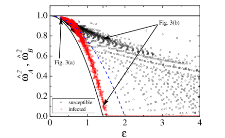
Figure 2: $\hat{\omega}_{A}^{2}$ and $\hat{\omega}_{B}^{2}$ for the same SI model as in Fig. 1. The points correspond to a uniform scanning of a portion of phase space: $b_{A}=b_{BA}=0.1$, $d_{A}\in(0,0.2)$, $d_{B}\in(0,0.5)$, $p\in(2d_{B},3.2)$. The full lines show the bounds of Eq. (12), while the dashed one corresponds to $\omega_{d}$. The arrows point to the values corresponding to the parameters used in Fig. 3.

It is straightforward to see that $\langle S_{A}(\omega)\rangle$ is either monotonically decreasing or it has a single maximum at

$$\hat{\omega}_{A}^{2}=-F_{A}+\sqrt{(F_{A}+1)^{2}-\epsilon^{2}F_{A}}.$$ (11)

The condition of positivity for the argument of the square root gives the region in phase space where the power spectrum has a single maximum. Notice that for $\epsilon<\sqrt{2}$ this condition is fulfilled regardless of the exact dependence of $F_{A}$ on the parameters of the model. It can also be proved that $\hat{\omega}_{A}^{2}$ satisfies risau07 :

$$1-\epsilon^{2}/2<\hat{\omega}_{A}^{2}<1$$ (12)

(these bounds seem to be tight). In particular, this implies that in all the possible stochastic models that lead to the same deterministic equations (same $C$’s, different $D$’s) the position of the maximum can only vary within a finite range, that shrinks with $\epsilon$.

For small $\epsilon$, $\hat{\omega}_{A}^{2}$ tends to $1$, which means that not only the frequencies of possible oscillations for both populations become close, but also that they become close to $\omega_{d}$, the frequency of the damped oscillations of the deterministic model (which also tends to 1 as $\epsilon\to 0$). It is in this regime that the populations show the coherent dynamics characteristic of stochastic oscillations. This motion will be further characterized below by the quality of the spectrum peak. Figure 2 shows $\hat{\omega}^{2}_{A}$ and $\hat{\omega}^{2}_{B}$ as functions of $\epsilon$ for the SI model presented in Fig. 1, for a wide range of system parameters. The bounds given by Eq. (12) are shown by continuous lines. Each point represents the normalized squared frequency for one set of parameters, for both populations. The deterministic frequency, $\omega_{d}$, is also shown, to emphasize the difference between the three frequencies present in the system.

When $\sqrt{2}<\epsilon<2$ there can be some stochastic models for which no peak is present in $S(\omega_{A})$ or $S(\omega_{B})$. And, for some values of $F_{A}$ or $F_{B}$, it can happen that the power spectrum of any population has a maximum even if $\epsilon>2$, i.e. even when the deterministic system does not display damped oscillations (see Fig. 2: all the points to the right of $\epsilon\!=\!2$ correspond to systems with a peak in the spectrum of the susceptible (A) population, no peak in the infected (B) one, and no damped oscillations in the deterministic model). These two features show that the peaks of the stochastic power spectrum on the one hand, and the deterministic damped oscillations on the other, are not necessarily closely related.

The above discussion establishes the conditions for the existence of a peak in the power spectrum of one or both populations. That is, for the existence of a preferred frequency in their dynamics. But, should all peaks in the power spectrum be regarded as “oscillations”? The answer to this question is certainly negative, and leads one to look for a criterion to quantify how close a time series is to an oscillatory movement. This can be done by defining the “quality” of the oscillation as a measure of the sharpness of the peak. We propose one such measure in the following.

Given a power spectrum of the form (9) we define the quality of a peak at $\omega_{peak}$ as

$$Q_{A}(\omega)=\frac{\omega_{peak}\langle S_{A}(\omega_{peak})\rangle}{\int\langle S_{A}(\omega)\rangle d\omega}.$$ (13)

This quantity is dimensionless and scale invariant. It is related to Fisher’s kappa, which measures the non-stationarity of a signal, given its periodogram fisher29 . For functions with only one peak, $Q_{A}$ increases as the peaks grows. For power spectra of the form (9), $Q_{A}$ can be readily calculated (using that $\int\langle S_{A}(\omega)\rangle d\omega=\langle\xi_{A}^{2}\rangle$, see vankampen ):

$$Q_{A}(\omega_{A})=\frac{\hat{\omega}_{A}\epsilon}{(\hat{\omega}_{A}^{2}-1)^{2}+\hat{\omega}_{A}^{2}\epsilon^{2}}\left(\frac{F_{A}+\hat{\omega}_{A}^{2}}{F_{A}+1}\right).$$ (14)

The quality $Q_{A}$ diverges as $\epsilon$ vanishes, regardless of the exact dependence of $F_{A}$ on the parameters of the model. Therefore, one can assure that the corresponding time series will look oscillatory when $\epsilon$ is sufficiently small (see Fig. 3 for an example of this). In such a case, we have already shown that the frequencies of both populations are very close, and also very close to the frequency of the deterministic damped oscillations.

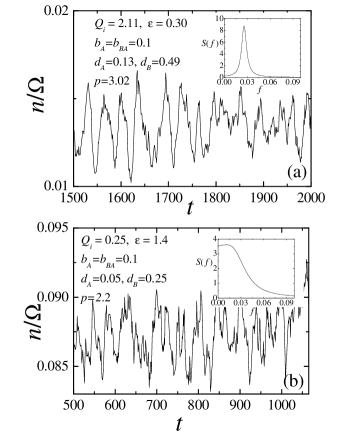
Figure 3: Two stochastic realizations of the SI model, with different qualities. The insets show the corresponding analytical average power spectra. Only the infected population is shown. The arrows in Fig. 2 point to the corresponding frequencies: $\omega_{A}\sim\omega_{B}\sim\omega_{d}$ for the good quality case shown in (a), and $\omega_{A}\gg\omega_{B}$ for the bad quality one shown in (b). $\Omega=10^{5}$.

Could it also happen that, for large values of $\epsilon$, when the frequencies of populations $A$ and $B$ can be rather different, one gets very sharp peaks? It can be shown that this is not the case by giving bounds of $Q_{A}$ that depend solely on $\epsilon$ risau07 :

$$\frac{2}{\pi\epsilon}\left(\frac{1-\epsilon^{2}/2}{1+\epsilon^{2}/4}\right)<Q_{A}(\omega)<\frac{2}{\pi\epsilon}.$$ (15)

The upper bound shows that, when $\epsilon$ is not small, the peak cannot be arbitrarily sharp. On the other hand, the lower bound shows that, when $\epsilon$ is small the peak is sharp for all the stochastic counterparts of a deterministic model. In Fig. 4 we illustrate this by showing several values of $Q_{A}$ and $Q_{B}$ for the SI model, along with the corresponding bounds.

One practical question remains: what is the critical quality value above which one can be sure that the time series will indeed “look” oscillatory? As it is to be expected, the continuous nature of $Q$ precludes a conclusive answer. From exhaustive observations of different models we find that when $Q(\omega_{peak})>1$, the oscillations are well defined and notably different from a noisy evolution (see Fig. 4).

In summary, we have shown that, by defining a quality measure, one can quantify the “oscillatory look” of a time series. Interestingly, we find that oscillations are present only when $\epsilon$ is small. This means that, given a deterministic model, one can know, using the bounds (15), whether the time series given by any stochastic counterpart of the model will look oscillatory or not. In addition, we have shown that, when oscillations are clear, the corresponding frequencies of both populations will be close to each other and to the frequency of the damped oscillation of the deterministic system.

Given that our conclusions are based on the analysis of the first two terms of the systematic van Kampen’s expansion of the master equation, they are exact only in the limit $\Omega\to\infty$. These analytical results, nevertheless, compare well with the numerical observations made on finite systems. More details about the validity of the expansion for finite systems will be given elsewhere risau07 .

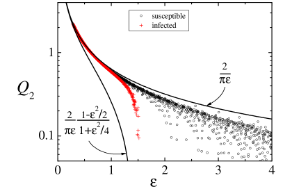
Figure 4: $Q_{A}$ and $Q_{B}$ as functions of $\epsilon$ for the SI model of Fig. 1. The points correspond to the same portion of phase space as in Fig. 2. The lines show the upper and lower bounds of Eq. (15).

- (1) M. Begon, C. R. Townsend and J. L. Harper, Ecology: From Individuals to Ecosystems (Blackwell, 2006).
- (2) E. B. Wilson and O. M. Lombard, Pathology 31, 367 (1945).
- (3) I. Prigogine and R. Lefever, J. Chem. Phys. 48, 1695 (1968).
- (4) E. Renshaw, Modelling Biological Populations in Space and Time, (Cambridge, 1991). See Sections 6.2 and 10.4.
- (5) M. S. Bartlett, J. R. Stat. Soc. A 120, 48 (1957).
- (6) H. W. Hethcote and S. A. Levin, in Applied Mathematical Ecology, L. Gross, T. G. Hallam and S.A. Levin, (eds.), pp. 193-211 (Springer, Berlin, 1989).
- (7) J. P. Aparicio and H. G. Solari, Math. Biosciences 169, 15 (2001).
- (8) A. J. McKane and T. J. Newman, Phys. Rev. Lett. 94, 218102 (2005).
- (9) N. G. van Kampen, Stochastic Processes in Physics and Chemistry (Elsevier Sience B.V., Amsterdam, 2003).
- (10) A. J. McKane and T. J. Newman, Phys. Rev. E 70, 041902 (2004).
- (11) R. A. Fisher, Proc. R. Soc. Lon. A 125, 54 (1929).
- (12) S. Risau-Gusman and G. Abramson, in preparation.