Stochastic dynamics of a finite-size spiking neural network

Abstract

We present a simple Markov model of spiking neural dynamics that can be analytically solved to characterize the stochastic dynamics of a finite-size spiking neural network. We give closed-form estimates for the equilibrium distribution, mean rate, variance and autocorrelation function of the network activity. The model is applicable to any network where the probability of firing of a neuron in the network only depends on the number of neurons that fired in a previous temporal epoch. Networks with statistically homogeneous connectivity and membrane and synaptic time constants that are not excessively long could satisfy these conditions. Our model completely accounts for the size of the network and correlations in the firing activity. It also allows us to examine how the network dynamics can deviate from mean-field theory. We show that the model and solutions are applicable to spiking neural networks in biophysically plausible parameter regimes.

I Introduction

Neurons in the cortex, while exhibiting signs of synchrony in certain states and tasks Singer and Gray (1995); Steinmetz et al. (2000); Fries et al. (2001); Pesaran et al. (2002), mostly fire stochastically or asynchronously Softky and Koch (1993). Previous theoretical and computational work on the stochastic dynamics of neuronal networks have mostly focused on the behavior of networks in the infinite size limit with and without the presence of external noise. The bulk of these studies utilize a mean-field theory approach, which presumes self-consistency between the input to a given neuron from the collective dynamics of the network with the output of that neuron and either ignores fluctuations or assumes that the fluctuations obey a prescribed statistical distribution, e.g. Amit and Brunel (1997a, b); Van Vreeswijk and Sompolinsky (1996, 1998); Gerstner (2000); Cai et al. (2004) and Gerstner and Kistler (2002a) for a review. Within the mean-field framework, the statistical distribution of fluctuations may be directly computed using a Fokker-Planck approach Abbott and Vreeswijk (1993); Treves (1993); Fusi and Mattia (1999); Golomb and Hansel (2000); Brunel (2000a); Nykamp and Tranchina (2000); Hansel and Mato (2003); Del Giudice and Mattia (2003); Brunel and Hansel (2006) or estimated from the response of one individual neuron submitted to noise Plesser and Gerstner (2000); Salinas and Sejnowski (2002); Fourcaud and Brunel (2002); Soula et al. (2006).

Although, correlations in mean-field or near mean-field networks can be nontrivial Ginzburg and Sompolinsky (1994); Van Vreeswijk and Sompolinsky (1996, 1998); Meyer and Van Vreeswijk (2002), in general, mean-field theory is strictly valid only if the size of the network is large enough, the connections are sparse enough or the external noise is large enough to decorrelate neurons or suppress fluctuations. Hence, mean-field theory may not capture correlations in the firing activity of the network that could be important for the transmission and coding of information.

It is well known that finite-size effects can contribute to fluctuations and correlations Brunel (2003b). It could be possible that for some areas of the brain, small regions are statistically homogeneous in that the probability of firing of a given neuron is mostly affected by a common input and the neural activity within a given neighborhood. These neighborhoods may then be influenced by finite-size effects. However, the effect of finite size on neural circuit dynamics is not fully understood. Finite-size effects have been considered previously using expansions around mean-field theory Ginzburg and Sompolinsky (1994); Meyer and Van Vreeswijk (2002); Mattia and del Giudice (2002). It would be useful to develop analytical methods that could account for correlated fluctuations due to the finite size of the network away from the mean-field limit.

In general, finite-size effects are difficult to analyze. We circumvent some of the difficulties by considering a simple Markov model where the firing activity of a neuron at a given temporal epoch only depends on the activity of the network at a previous epoch. This simplification, which presumes statistical homogeneity in the network, allows us to produce analytical expressions for the equilibrium distribution, mean, variance, and autocorrelation function of the network activity (firing rate) for arbitrary network size. We find that mean-field theory can be used to estimate the mean activity but not the variance and autocorrelation function. Our model can describe the stochastic dynamics of spiking neural networks in biophysically reasonable parameter regimes. We apply our formalism to three different spiking neuronal models.

II The model

We consider a simple Markov model of spiking neurons. We assume that the network activity, which we define as the number of neurons firing at a given time, is characterized entirely by the network activity in a previous temporal epoch. In particular, the number of neurons that fire between $t$ and $t+\Delta t$ only depends on the number that fired between $t-\Delta t$ and $t$. This amounts to assuming that the neurons are statistically homogeneous in that the probability that any neuron will fire is uniform for all neurons in the network and have a short memory of earlier network activity. Statistical homogeneity could arise for example, if the network receives common input and the recurrent connectivity is effectively homogeneous. We note that our model does not necessarily require that the network architecture be homogeneous, only that the firing statistics of each neuron be homogeneous. As we will show later, the model can, in some circumstances, tolerate random connection heterogeneity. Short neuron memory can arise if the membrane and synaptic time constants are not excessively long.

The crucial element for our formalism is the gain or response function of a neuron $p(i,t)$, which gives the probability of firing of one neuron within $t$ and $t+\Delta t$ given that $i$ neurons have fired in the previous epoch. The time dependence can reflect the time dependence of an external input or a network process such as adaptation or synaptic depression. Without loss of generality, we can rescale time so that $\Delta t=1$.

Assuming $p(i,t)$ is the same for all neurons, then the probability that exactly $j$ neurons in the network will fire between $t$ and $t+1$ given that $i$ neurons fired between $t-1$ and $t$ is

$$p(X(t+1)=j|X(t)=i)=C_{N}^{j}p(i,t)^{j}(1-p(i,t))^{N-j},$$ (1)

where $X(t)$ is the number of neurons firing between $t-1$ and $t$ and $C_{N}^{k}$ is the binomial coefficient. Equation (1) describes a Markov process on the finite set $\{0,..,N\}$ where $N$ is the maximum number of neurons allowed to fire on a time interval $\Delta t$. The process can be re-expressed in terms of a time dependent probability density function (PDF) of the network activity $P(t)$ and a Markov transition matrix (MTM) defined by

$$M_{ij}(t)\equiv p(X(t+1)=j|X(t)=i)=C_{N}^{k}p(i,t)^{j}(1-p(i,t))^{N-j}.$$ (2)

$P(t)$ is a row vector on the space $[0,1]^{N}$ that obeys

$$P(t+1)=P(t)M(t)$$ (3)

For time invariant transition probabilities, $p(i,t)=p(i)$ and for fixed $N$, we can write

$$P(t)=P(0)M^{t}.$$ (4)

Our formalism is a simplified variation of previous statistical approaches, which use renewal models for neuronal firing Gerstner and Hemmen (1992); Gerstner (1995); Meyer and Van Vreeswijk (2002). In those approaches, the probability for a given neuron to fire depends on the refractory dynamics and inputs received over the time interval since the last time that particular neuron fired. Our model assumes that the neurons are completely indistinguishable so the only relevant measure of the network dynamics is the number of neurons active within a temporal epoch. Thus the probability of a neuron to fire depends only on the network activity in a previous temporal epoch. This simplifying assumption allows us to compute the PDF of the network activity, the first two moments, and the autocorrelation function analytically.

III Time independent Markov model

We consider a network of size $N$ with a time independent response function, $p(i,t)=p(i)$, so that (4) specifies the temporal evolution of the PDF of the network activity. If $0<p(i)<1$ for all $i\in[0,N]$ (i.e. the probability of firing is never zero nor one), then the MTM is a positive matrix (i.e. it has only non-zero entries). The sum over a row of the MTM is unity by construction. Thus the maximum row sum matrix norm of the MTM is unity implying that the spectral radius is also unity. Hence, by the Frobenius-Perron Theorem, the maximum eigenvalue is unity and it is unique. This implies that for all initial states of the PDF, $P(t)$ converges to a unique left eigenvector $\mu$ called the invariant measure, which satisfies the relation

$$\mu=\mu M.$$ (5)

The invariant measure is the attractor of the network dynamics and the equilibrium PDF. Given that the spectral radius of $M$ is unity, convergence to the equilibrium will be exponential at a rate governed by the penultimate eigenvalue. We note that if the MTM is not positive then there may not be an invariant measure. For example if the probability of just one possible transition is zero, then the PDF may never settle to an equilibrium.

The PDF specifies all the information of the system and can be found by solving (5). From (4), we see that the invariant measure is given by the column average over any arbitrary PDF of $\lim_{t\rightarrow\infty}M^{t}$. Hence, the infinite power of the MTM must be a matrix with equal rows, each row being the invariant measure. Thus, a way to approximate the invariant measure to arbitrary precision is to take one row of a large power of the MTM. The higher the power, the more precise the approximation. Since the convergence to equilibrium is exponential, a very accurate approximation can be obtained easily.

III.1 Mean and variance

In general, of most interest are the first two moments of the PDF so we derive expressions for the expectation value and variance of any function of the network activity. Let $X\in[0,...N]$ be a random variable representing the network activity and $f$ be a real valued function of $X$. The expectation value and variance of $f$ at time $t$ is thus

$$\langle f(X)\rangle_{t}=\sum_{k=0}^{N}f(k)P_{k}(t)$$ (6)

and

$$Var_{t}(f(X))=\langle f(X)^{2}\rangle_{t}-\langle f(X)\rangle_{t}^{2}.$$ (7)

where we denote the $k$th element of vector $P(t)$ by $P_{k}(t)$. We note that in numerical simulations, we will implicitly assume ergodicity at equilibrium. That is, we will consider that the expectation value over all the possible outcomes to be equal to the expectation over time.

Inserting (2) into (3) and using the definition of the mean of a binomial distribution, the mean activity $\langle X\rangle_{t}$ has the form

$$\langle X\rangle_{t}=N\langle p(X)\rangle_{t-1}.$$ (8)

The mean firing rate of the network is $\langle X\rangle_{t}/\Delta t$. We can also show that the variance is given by

$$Var_{t}(X)=N\langle p(1-p)\rangle_{t-1}+N^{2}Var_{t-1}(p).$$ (9)

Details of the calculations for the mean and variance are in Appendix A. Thus the mean and variance of the network activity are expressible in terms of the mean and variance of the response function. At equilibrium, (8) and (9) are $\langle X\rangle_{\mu}=N\langle p\rangle_{\mu}$ and $Var_{\mu}(X)=N\langle p(1-p)\rangle_{\mu}+N^{2}Var_{\mu}(p)$, respectively. Given an MTM, we can calculate the invariant measure and then from that obtain all the moments.

If we suppose the response function to be linear, we can compute the mean and variance in closed-form. Consider the linear response function

$$p(X)=p_{0}+\frac{(q-p_{0})}{Nq}X$$ (10)

for $X\in[0,N]$. Here $p_{0}\in[0,1]$ is the probability of firing for no inputs and $(q-p_{0})/Nq$ is the slope of the response function. Inserting (10) into (8), gives

$$\langle X\rangle_{\mu}=Np_{0}+\frac{(q-p_{0})}{q}\langle X\rangle_{\mu}.$$ (11)

Solving for $\langle X\rangle_{\mu}$ gives the mean activity

$$\langle X\rangle_{\mu}=Nq,$$ (12)

Substituting (10) into (9) leads to the variance

$$Var_{\mu}(X)=N\frac{q(1-q)}{1-\lambda^{2}+\lambda^{2}/N}$$ (13)

where $\lambda=(q-p_{0})/q$. The details of these calculations are given in Appendix A.

The expressions for the mean and variance give several insights into the model. From (10), we see that the mean activity (12) satisfies the condition

$$p(Nq)=q.$$ (14)

Hence, on a graph of the response function versus the input, the mean response probability is given by the intersection of the response function and a line of slope $1/N$, which we denote the diagonal. Using (12), (14) can be re-expressed as

$$\langle X\rangle_{\mu}=Np(\langle X\rangle_{\mu})$$ (15)

In equilibrium, the mean response of a neuron to $\langle X\rangle$ neurons firing is $\langle X\rangle/N$. Hence, for a linear response function, the mean network activity obeys the self-consistency condition of mean-field theory. This can be expected because of the assumption of statistical homogeneity.

The variance (13) does not match a mean-field theory that assumes uncorrelated statistically independent firing. In equilibrium, the mean probability to fire of a single neuron in the network is $q$. Thus, each neuron obeys a binomial distribution with variance $q(1-q)$. Mean-field theory would predict that the network variance would then be given by $Nq(1-q)$. Equation (13) shows that the variance exceeds the statistically independent result by a factor that is size dependent, except for $q=p_{0}$, which corresponds to an unconnected network. Hence, the variance of the network activity cannot be discerned from the firing characteristics of a single neuron. The network could possess very large correlations while each constituent neuron would exhibit uncorrelated firing.

When $N>>\lambda^{2}$, the variance scales as $N$ but for small $N$, there is a size-dependent correction. The coefficient of variation approaches zero as $1/\sqrt{N}$ as $N$ approaches infinity. When $\lambda=1$, the slope of the response function is $1/N$ and coincides with the diagonal. This is a critical point where the equilibrium state becomes a line attractor Seung (1996). In the limit of $N\rightarrow\infty$, the variance diverges at the critical point. At criticality, the variance of our model has the form $N^{2}q(1-q)$, which diverges as the square of $N$. Away from the critical point, in the limit as $N$ goes to infinity, the variance has the form $(Nq(1-q))/(1-\lambda^{2})$. Thus, the deviation from mean-field theory is present for all network sizes and becomes more pronounced near criticality.

The mean-field solution of (14) is not a strict fixed point of the dynamics (4) per se. For example, if the response function is near criticality, possesses discontinuities, or crosses the diagonal multiple times then the solution of (14) may not give the correct mean activity. Additionally, if the slope of the crossing has a magnitude greater than $1/N$, then the crossing point would be “locally unstable”. Consider, small perturbations of the mean around the fixed point given by (12)

$$\langle X\rangle_{t}=Nq+v(t)$$ (16)

The response function (10) then takes the form

$$p(X)=q+\frac{\lambda}{N}v$$ (17)

where $\lambda=(q-p_{0})/q$. Substituting (16) and (17) into (8) gives

$$\langle v\rangle_{t}=\lambda\langle v\rangle_{t-1}$$ (18)

Hence, $v$ will approach zero (i.e. fixed point is stable) only if $|\lambda|<1$.

Finally, we note that in the case that there is only one solution to (14) (i.e. response function crosses the diagonal only once), if the function is continuous and monotonic then it can only cross with $\lambda<1$ (slope less than $1/N$) since $0<p<1$. Thus, a continuous monotonic increasing response function that crosses the diagonal only once, has a stable mean activity given by this crossing. This mean activity corresponds to the mode of the invariant measure.

We can estimate the mean and variance of the activity for a smooth nonlinear response function that crosses the diagonal once by linearizing the response function around the crossing point ($q=p(Nq)$). Hence, near the intersection

$$p(X)=q+\lambda\frac{(X-Nq)}{N}.$$ (19)

where $\lambda=N\frac{\partial p}{\partial X}(Nq)$. Using (12) and (13) then gives

$$\langle X\rangle_{\mu} = Nq$$ (20)

$$Var_{\mu}(X) = \frac{Nq(1-q)}{1-\lambda^{2}+\lambda^{2}/N}$$ (21)

Additionally, the crossing point is stable if $|\lambda|<1$. These linearized estimates are likely to break down near criticality (i.e. $\lambda$ near one).

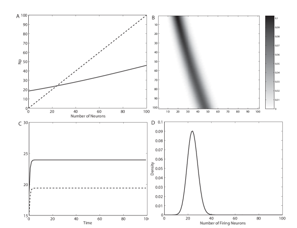
Figure 1: Example for response function $p(n)=\frac{1}{2\pi}\int_{\frac{\theta-I-Jn}{\sigma}}^{\infty}e^{-\frac{x^{2}}{2}}dx$ with $N=100$, $\theta=1$, $I=0.1$, $J=1.5/N$ and $\sigma=1.0$. A) $Np(n)$ (solid line) and the diagonal (dashed line). B) The associated Markov Transition Matrix (in gray levels). C) The evolution of the mean network activity (solid line) and the variance (dashed line). The steady-state is quickly reached and the activity corresponds to the crossing point between $Np(n)$ and the diagonal. D) The invariant measure (i.e the PDF of the network activity).

We show an example of a response function and resulting MTM in Figure 1. Starting with a trivial density function (all neurons are silent), we show the time evolution of the mean and the variance in figure 1C. We show the invariant measure in figure 1D. The equilibrium state is given by the intersection of the response function with the diagonal. We see that the mode of the invariant measure is aligned with the mean activity given by the crossing point.

III.2 Autocovariance and autocorrelation functions

We can also compute the autocovariance function of the network activity:

$$\rm{Cov}(\tau)=\langle(X(t)-\langle X\rangle_{\mu})(X(t+\tau)-\langle X\rangle_{\mu})\rangle=\langle X(t)X(t+\tau)\rangle-\langle X^{2}\rangle_{\mu}.$$ (22)

Noting that

$$\langle X(t)X(t+\tau)\rangle=\sum_{j}\sum_{k}jkp(X(t+\tau)=k|X(t)=j)p(X(t)=j)$$ (23)

where $p(X(t+\tau)=k|X(t)=j)=M_{jk}^{\tau}$, we show in Appendix B, that at equilibrium

$$\rm{Cov}(\tau)=\lambda^{\tau}Var_{\mu}(X)$$ (24)

where $\lambda$ is the slope factor ($N$ times the slope) of the response function evaluated at the crossing point with the diagonal. The autocorrelation function $AC(\tau)$ is simply $\lambda^{\tau}$.

The correlation time is given by $1/\ln\lambda$. At the critical point ($\lambda=1$), the correlation time becomes infinite. For a totally decorrelated network, $\lambda=0$, giving a Kronecker delta function for the autocorrelation as expected. For an inhibitory network ($\lambda<0$), the autocorrelation exhibits decaying oscillations with period equal to the time step of the Markov approximation (i.e. $\rm{Cov}(1)<0$). (Since we have assumed $p>0$, an inhibitory network in this formalism is presumed to be driven by an external current and the probability of firing decreases when other neurons in the local network fire.) We stress that these correlations are only apparent at the network level. Unless the rate is very high, a single neuron will have a very short correlation time.

III.3 Multiple Crossing Points

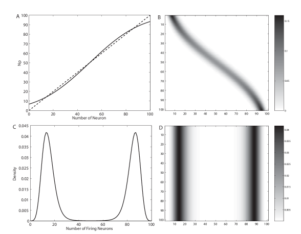
Figure 2: Example where the response function crosses the diagonal three times. A) $Np(n)$ (solid line) and diagonal (dashed line). B) The associated MTM. C) The invariant measure. D) MTM${}^{10^{5}}$. All rows are equal to the invariant measure. Parameters are $N=100$, $I=0.1$, $J=1.8/N$ and $\sigma=0.6$.

For dynamics where $0<p<1$, if the response function is continuous and crosses the diagonal more than once, then the number of crossings must be odd. Consider the case with three crossings with $p(0)<p(N)$. If the slopes of all the crossings are positive (i.e. a sigmoidal response function), then the slope factor $\lambda$ of the middle crossing will be greater than one while the other two crossings will have $\lambda$ less than one implying two stable crossing points and one unstable one in the middle. Figure 2A and B provide an example of such a response function and its associated MTM. The invariant measure is shown in figure 2C. We see that it is bimodal with local peaks at the two crossing points with $\lambda$ less than one. The invariant measure is well approximated by any row of a large power of the MTM (figure 2D). If the stable crossing points are separated enough (beyond a few standard deviations), then we can estimate the network mean and variance by combining the two local mean and variances. Assuming that the stable crossing points are $q_{1}$ and $q_{2}$ ($q_{1}<q_{2}$) with slope factors $\lambda_{1}$ and $\lambda_{2}$. Then the mean and the variance are:

$$\langle X\rangle_{\mu} = N\frac{q_{1}+q_{2}}{2}$$ (25)

$$Var_{\mu}(X) = \frac{N}{2}\left(\frac{q_{1}(1-q_{1})}{1-\lambda_{1}^{2}+\lambda_{1}^{2}/N}+\frac{q_{2}(1-q_{2})}{1-\lambda_{2}^{2}+\lambda_{2}^{2}/N}\right)+N^{2}\left(\frac{q_{1}-q_{2}}{2}\right)^{2}$$ (26)

IV Fast leak spiking model

We now consider a simple neuron model where the firing state obeys

$$V_{i}(t)=\rm{H}(I(t)+\frac{1}{N}\sum_{k=1}^{N}J_{ik}V_{k}(t-1)+S(t)-\theta)$$ (27)

where $\rm{H}(\cdot)$ is the Heaviside step function, $I(t)$ is an input current, $S(t)=N(0,\sigma)$ is uncorrelated Gaussian noise, $\theta$ is a threshold, and $J_{ik}$ is the connection strength between neurons in the network. When the combined input of the neuron is below threshold, $V_{i}=0$ (neuron is silent) and when the input exceeds threshold, $V_{i}=1$ (neuron is active). This is a simple version of a spike response or renewal model Gerstner and Hemmen (1992); Gerstner (1995); Meyer and Van Vreeswijk (2002).

In order to apply our Markov formalism, we need to construct the response function. We assume first that the connection matrix has constant entries $J$. We will also consider disordered connectivity later. The response function is the probability that a neuron will fire given that $n$ neurons fired previously. The response function at $t$ for the neuron is then given by

$$p(n,t)=\frac{1}{\sqrt{2\pi}}\int_{\frac{\theta-I(t)-nJ/N}{\sigma}}^{\infty}e^{-x^{2}/2}dx$$ (28)

If we assume a time independent input then we can construct the MTM using (2). The equilibrium PDF is given by (5), and can be approximated by one row of a large power of the MTM.

IV.1 Mean, variance and autocorrelation

Imposing the self-consistency condition (14) on the mean activity $Nq$, where $q=\langle p\rangle_{\mu}$, and $p$ is given by (28) leads to

$$q=\frac{1}{\sqrt{2\pi}}\int_{\frac{\theta-I-qJ}{\sigma}}^{\infty}e^{-x^{2}/2}dx.$$ (29)

Taking the derivative of $p(n,t)$ in (28) at $n=Nq$ gives

$$\lambda=\frac{J}{\sigma\sqrt{2\pi}}e^{-\frac{{(\theta-I-Jq)}^{2}}{2\sigma^{2}}}.$$ (30)

Using this in (21) gives the variance.

Equation (30) shows the influence of noise and recurrent excitation on the slope factor and hence variance of the network activity. For $\lambda<1$, the variance (21) increases with $\lambda$. An increase in excitation $J$ increases $\lambda$ for large $J$ but decreases $\lambda$ for small $J$. Similarly, a decrease in noise $\sigma$ increases $\lambda$ for large $\sigma$ but decreases it for small $\sigma$. Thus, variability in the system can increase or decrease with synaptic excitation and external noise depending on the regime. The autocovariance function, from (24) is

$$Cov(\tau)=\lambda^{\tau}\frac{Nq(1-q)}{1-\lambda^{2}+\lambda^{2}/N}.$$ (31)

IV.2 Bifurcation diagram

Bifurcations occur when the stability of the mean-field solutions (i.e. crossing points) for the mean activity changes. We can construct the bifurcation diagram on the $I-J$ plane by locating crossing points where $\lambda=1$. We first consider rescaled parameters $\mathcal{I}=(\theta-I)/\sigma$ and $\mathcal{J}=J/\sigma$. Then (29) becomes

$$q=\frac{1}{\sqrt{2\pi}}\int_{\mathcal{I}-q\mathcal{J}}^{\infty}e^{-x^{2}/2}dx$$ (32)

and (30) becomes

$$\lambda=\frac{\mathcal{J}}{\sqrt{2\pi}}e^{-\frac{{(\mathcal{I}-\mathcal{J}q)}^{2}}{2}}$$ (33)

Solving (33) for $q$ and inserting into (32) gives

$$\mathcal{I}=\frac{\mathcal{J}}{\sqrt{2\pi}}\int_{\pm\sqrt{\ln(\frac{\mathcal{J}^{2}}{2\pi\lambda^{2}})}}^{\infty}e^{-x^{2}/2}dx\pm\sqrt{\ln(\frac{\mathcal{J}^{2}}{2\pi\lambda^{2}})}$$ (34)

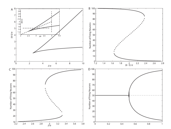
Figure 3: A) The two dimensional bifurcation diagram ($\lambda=1$) as a function of $\frac{\theta-I}{\sigma}$ and $\frac{J}{\sigma}$. Inset: the traversal lines of the various one dimensional bifurcation diagrams shown in B) vertical, C) horizontal and D) oblique.

The bifurcation points are obtained by setting $\lambda=1$ in (34) and evaluating the integral. The solutions have two branches that satisfy the conditions $\mathcal{J}\geq\sqrt{2\pi}$ and $\mathcal{I}\geq\sqrt{\pi/2}$. Figure 3A shows the two dimensional bifurcation diagram on the $\mathcal{I}-\mathcal{J}$ plane. The intersection of the two branches at $\mathcal{J}=\sqrt{2\pi}$ and $\mathcal{I}=\sqrt{\frac{\pi}{2}}$ is a co-dimension two cusp bifurcation point (i.e. satisfies $Np^{\prime}(x)=1$, $Np^{\prime\prime}(x)=0$ with genericity conditions Kuznetsov (1998)). Between the two branches there are three crossing points (two of which are stable), outside there is one stable crossing point. Each traversal of a branch yields a saddle node bifurcation as seen in figures 3B and C for the vertical and horizontal traversals (shown in the inset to figure 3A) respectively. Traversing through the critical point along the diagonal line in the inset of figure 3A shows a pitchfork bifurcation. We have assumed that $J>0$ (i.e excitatory network). By taking $J\rightarrow-J$ we obtain the same bifurcation diagram for the inhibitory case and the above conditions still hold using the absolute value of $J$.

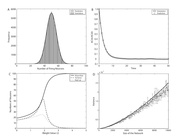
Figure 4: A) Numerical and theoretical PDF of the network activity at equilibrium for $N=100$, $\theta=1$, $I=0.1$, $\sigma=0.8$ and $J=1.8$. The theoretical PDF was obtained by taking one row of $MTM^{100}$. B) Numerical and theoretical autocorrelation function for same parameters as A). Solid line is $\lambda^{t}$ with the predicted $\lambda$ from equation (30). C) Dependence of the mean (solid line) and variance (dashed line) with $J$. The mean-field variance is $Nq(1-q)$ (dotted line). D) Evolution of the variance when $\lambda=1$ versus $N$ for $I=1-\sqrt{2\pi}$, $J=\sqrt{2\pi}$, $\sigma=1$, $\theta=1$. The solid line is $N^{3/2}q(1-q)$.

We compare our analytical estimates from the Markov model with numerical simulations of the fast leak model (27) in figure 4. Figure 4A shows that the equilibrium PDF derived from the MTM matches the PDF generated from the simulation. Figure 4B shows a comparison of $\lambda^{\tau}$ versus the simulation autocorrelation function. Figure 4C shows the mean and variance of the activity versus the connection weight $J$. The theoretical results match the simulation results very well. On the same plot, we show the mean-field theory estimate where the neurons are assumed to be completely uncorrelated. For low recurrent excitation and hence low activity, the correlations can be neglected and the system behaves like an uncorrelated neural network. However, as the excitation and firing activity increase, correlations become more significant and the variance grows quicker than the uncorrelated result. For very strong connections, the firing activity saturates and the variance drops. In that case, mean-field theory is again an adequate approximation. Figure 4D shows the variance versus $N$ for a network at the critical point, $\mathcal{J}=\sqrt{2\pi}$ and $\mathcal{I}=\sqrt{\frac{\pi}{2}}$ where $\lambda=1$ at the crossing point. We see that the variance grows approximately as $N^{3/2}$. This is faster than the mean-field result but slower than the prediction for a linear response function. The breakdown of the linear estimate is expected near criticality.

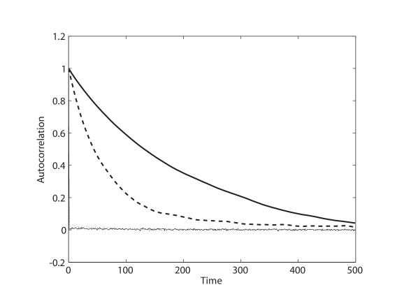
Figure 5: Autocorrelation of the network and one neuron at a critical point ($\lambda=1$). The solid line is for a network of 10,000 neurons and the dashed line is for a network of 1000 neurons. Crosses and dots are the autocorrelation of one neuron for $N=1000$ and $N=10,000$ respectively. The autocorrelation for one neuron decays almost immediately. Parameters are $\sigma=1$, $\theta=1$, $J=\sqrt{2\pi}$ and $I=1-\sqrt{2/\pi}$.

Figure 5 shows the simulation autocorrelation for both the network and one neuron (chosen randomly) for $N=1000$ and $N=10,000$. The parameters were chosen so the network was at a critical point ($\lambda=1$). We see that the correlation time of an individual neuron is near zero and much shorter than that of the network. With increasing $N$, we find that the correlation time increases for the network and decreases for the single neuron. Thus, a single neuron can be completely uncorrelated while the network has very long correlation times.

IV.3 Bistable regime

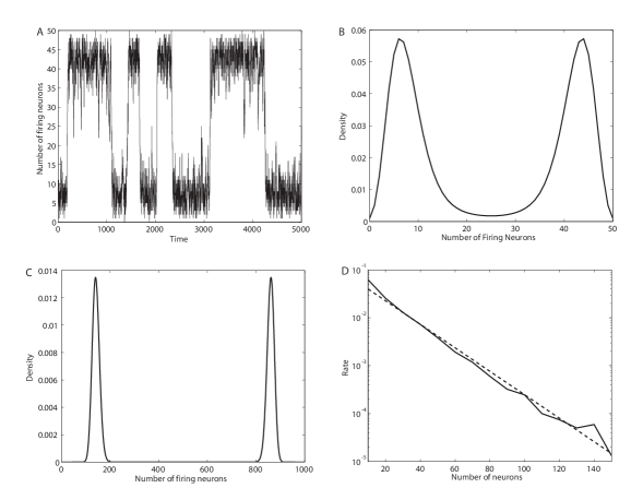
Figure 6: A) The firing activity over time of a bistable network of 50 neurons. The switching between the two states (high and low activity) is spontaneous. B) Theoretical PDF for $N=50$. C) Theoretical PDF for $N=1000$. D) Switching rate depends exponentially on $N$ (solid curve). Dashed line is a linear fit on semi-log scale. Parameters are: $J=1.8$, $\sigma=0.6$, $I=0.1$, $\theta=1$.

In the regime where there are three crossing points, the invariant measure is bimodal. Hence, the network activity is effectively bistable. Bistable network activity has been proposed as a model of working memory Compte et al. (2000); Laing and Chow (2001); Gutkin et al. (2001); Compte (2006). The two local equilibria are locally stable but due to the finite-size fluctuations, there can be spontaneous transitions from one state to the other. Figure 6A shows the activity over time for a bistable network with $N=50$. The associated PDF is shown in figure 6B. No external input has been added to the network. For $N=1000$, the switching rate is sufficiently low to be neglected. The resulting probability density function for this network is displayed on figure 6C.

We can estimate the scaling behavior on $N$ of the state switching rate and hence lifetime of a memory by supposing the finite-size induced fluctuations can be approximated by uncorrelated Gaussian noise. We can then map the switching dynamics to barrier hopping of a stochastically forced particle in a double potential well $V(x)$ with a stationary PDF given by the invariant measure $\mu$. The switching rate is given by the formula Risken (1989)

$$r=(2\pi)^{-1}\sqrt{V^{\prime\prime}(c)|V^{\prime\prime}(a)|}e^{-\frac{(V(a)-V(c))}{\sigma^{2}}}$$ (35)

where $V=-\sigma^{2}\ln(\mu)$, $\mu$ is the invariant measure, $c$ is a stable crossing point, $a$ is the unstable crossing point, and $\sigma^{2}$ is the forcing noise variance around $c$, which we take to be proportional to the variance of the network activity. For the general case, we cannot derive this rate analytically but we can obtain an estimate by assuming that the invariant measure is a sum of two Gaussian PDFs whose means are exactly the two stable crossing points.

$$\mu(x)=\frac{\exp\left(-\frac{(x-Nq_{1})^{2}}{2\sigma^{2}_{1}}\right)}{2\sqrt{2\pi}\sigma_{1}}+\frac{\exp\left(-\frac{(x-Nq_{2})^{2}}{2\sigma^{2}_{2}}\right)}{2\sqrt{2\pi}\sigma_{2}},$$ (36)

where $\sigma^{2}_{i}=\frac{Nq_{i}(1-q_{i})}{1-\lambda^{2}_{i}+\lambda^{2}_{i}/N}$ for $i=1,2$. Using this in (35) then gives

$$r\propto\Omega e^{-kN},$$ (37)

for a constant $k$. The switching rate is an exponentially decreasing function of $N$. We computed the switching rate for $N\in[0;150]$ for the parameters of the bistable network above. The results are displayed on figure 6D. For the parameters in 6D, a fit shows that $k$ is of order 0.05. For these parameters, switching between states will not be important when $N>>1/k\sim 20$.

IV.4 Disordered connectivity

We now consider the dynamics for disordered (random) connection weights $J_{ij}$ drawn from a Gaussian distribution ($N(\bar{J},\sigma^{2}_{J})$). Soula et al. (2006) showed that the input to a given neuron for a disordered network can be approximated by stochastic input. We thus choose random input drawn from the distribution, $N(k\bar{J},k\sigma^{2}_{J})$, for $k$ neurons having fired in the previous epoch. The response function (for time independent input) then obeys

$$p(n)=\frac{1}{\sqrt{2\pi}}\int_{\frac{\theta-I-n\bar{J}/N}{\sqrt{\sigma^{2}+n\sigma^{2}_{J}}/N}}^{\infty}e^{-x^{2}/2}dx.$$ (38)

Applying the self-consistency condition (14) for the mean firing probability $q$ gives

$$q=\frac{1}{\sqrt{2\pi}}\int_{\frac{\theta-I-q\bar{J}}{\sqrt{\sigma^{2}+q\sigma^{2}_{J}}}}^{\infty}e^{-x^{2}/2}dx$$ (39)

The variance is given by (21) with

$$\lambda=\frac{1}{\sqrt{2\pi}}\left(\frac{\bar{J}}{\sqrt{\sigma^{2}+q\sigma^{2}_{J}}}-\sigma^{2}_{J}\frac{\theta-I-q\bar{J}}{2(\sigma^{2}+q\sigma^{2}_{J})^{3/2}}\right)e^{-\frac{{(\theta-I-\bar{J}q)}^{2}}{2(\sigma^{2}+q\sigma^{2}_{J})}}$$ (40)

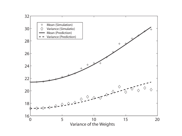
Figure 7: Mean (crosses) and variance (diamonds) from a numerical simulation of the fast leak model for $N=100$ neurons as a function of the variance of the random disordered connection weights. Theoretical mean (solid line) and variance (dashed line) match well with numerical simulation values. Parameters are $J=0.5/N$, $I=0.1$, $\sigma=1.0$, $\theta=1.0$.

Figure 7 shows the activity mean and variance as a function of the connection weight variance. There is a close match between the prediction and the results generated from a direct numerical simulation with 100 neurons. We note that a possible consequence of disorder in a neural network is a spin glass where many competing activity states could co-exist and so the resulting activity is strongly dependent on the initial condition Hopfield (1982). However, we believe that the stochastic forcing inherent in our network is large enough to overcome any spin glass effects. In the language of statistical mechanics, our system is at a high enough temperature to smooth the free energy function.

V Integrate-and-fire model

We now apply our formalism to a more biophysical integrate-and-fire model. We consider two versions. The first treats synaptic input as a current source and the second considers synaptic input in the form of a conductance change. We apply our Markov model with a discrete time step chosen to be the larger of the membrane or synaptic time constants.

V.1 Current-based synapse

We first consider an integrate-and-fire model where the synaptic input is applied as a current. The membrane potential obeys

$$\tau\frac{Dev_{i}}{dt}=I-V+\frac{J}{N}\sum_{t^{f}<t}^{N}\alpha(t-t^{f})+Z(t)$$ (41)

where $\alpha(t)=e^{-\frac{t}{\tau_{s}}}/\tau_{s}$ if $t>0$ and zero otherwise, $I$ is a constant input, $Z$ is an uncorrelated zero-mean white noise with variance $\sigma$, $J$ is the synaptic strength coefficient, $N$ is the network size, and $t^{f}$ are the firing times of all neurons in the network. These firing times are computed whenever the membrane potential crosses a threshold $V_{\theta}$, whereupon the potential is reset to $V_{Rs}$. After firing, neurons are prevented from firing during an absolute refractory period $r$. The parameter values are $\tau=1$ ms, $\tau_{s}=1$ ms,$V_{r}=-65$ mV, $V_{\theta}=-60$ mV, $V_{Rs}=-80$ mV and $r=1$ ms.

The network dynamics of this model had been studied previously in detail with a Fokker-Planck formalism Brunel (2000a); Brunel and Hansel (2006). These analyses showed that if the input current is an uncorrelated white noise $N(\mu_{I},\sigma_{I}^{2})$ and $\tau_{s}<1$ then the response function of the neuron in equilibrium is given by

$$\frac{1}{p(X)}=r+\sqrt{\pi}\int_{\frac{V_{r}-\mu_{I}-JX/N}{\sigma_{I}^{2}}}^{\frac{V_{\theta}-\mu_{I}-JX/N}{\sigma_{I}^{2}}}due^{u^{2}}(1+erf(u))$$ (42)

The mean activity is again given by $Nq$ where $\langle p(X)\rangle_{\mu}=q$, and $q$ is a solution of (14):

$$q=\left[r+\sqrt{\pi}\int_{\frac{V_{r}-\mu_{I}-Jq}{\sigma_{I}^{2}}}^{\frac{V_{\theta}-\mu_{I}-Jq}{\sigma_{I}^{2}}}due^{u^{2}}(1+erf(u))\right]^{-1}$$ (43)

Using (43), we can derive the slope factor $\lambda$,

$$\lambda=m^{2}\frac{J}{\sigma_{I}^{2}}\left(e^{(\frac{V_{\theta}-\mu_{I}-Jm}{\sigma_{I}^{2}})^{2}}(1+erf(\frac{V_{\theta}-\mu_{I}-Jm}{\sigma_{I}^{2}})-e^{(\frac{V_{r}-\mu_{I}-Jm}{\sigma_{I}^{2}})^{2}}(1+erf(\frac{V_{r}-\mu_{I}-Jm}{\sigma_{I}^{2}}))\right)$$ (44)

which can be used to estimate the variance using equation (21).

We also evaluate the response function numerically. We assume that the response function can be approximated by the firing probability of a neuron whose membrane potential obeys

$$\tau\frac{dV}{dt}=I+\frac{JX}{N}-V(t)+Z(t)$$ (45)

where $X\in\{0,...,N\}$. This presumes that the effect of discrete synaptic events can be approximated by a constant input equivalent to the mean input plus noise. We estimated the firing probability in a temporal epoch from the average firing rate of the neuron obeying (45) for each $X$. We used the firing probabilities directly to form the MTM. We then computed the equilibrium PDF, the mean activity (crossing point), the slope factor, and the variance. We choose the bin size of the Markov model to be the membrane time constant. All differential equations were computed using the Euler method with a time step of 0.01 ms.

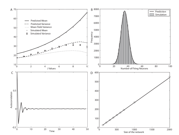
Figure 8: Current Synapse model – A) Mean (crosses) and variance (diamonds) versus $J$ from the numerical simulation compare well with the predictions (solid and dashed lines). The mean-field variance is also plotted (dotted line). Parameters are $N=100$, $I=4$, $\sigma=2.0$. B) The numerical PDF(histogram) and prediction (solid line) for $N=100$, $J=5.0$, $I=4$, and $\sigma=2.0$. C) The autocorrelation (solid line) for a network of $N=1000$. The dashed line is the estimated exponential decay with $\lambda=Cov(1)/Var$ (see text). Parameters are $J=5$, $I=4$, $\sigma=2.0$ and $\lambda=0.40$. D) The variance (circles) versus $N$. The solid line is from equation (21) with $\lambda$ computed using the autocorrelation decay for $N=1000$ ($\lambda=0.4$) displayed in C). Parameters are $J=5$, $I=4$, $\sigma=2.0$.

We compared the numerically simulated mean and variance of the network activity at equilibrium for 100 neurons with our theoretical predictions for differing synaptic strength $J$. The results are displayed in figure 8A. A close match is observed for both quantities. The mean and variance increase with $J$. Figure 8A also shows the mean-field (uncorrelated) variance. We see that the network variance always exceeds the mean-field value especially for midrange values of $J$. The PDFs from the numerical simulation of 100 neurons and using the Markov model are shown in 8B. The simulated PDF was generated by taking a histogram of the network activity over $10^{5}$ ms. For the Markov model, the PDF is the eigenvector with eigenvalue one and approximated by taking a single row of the one hundredth power of the MTM.

The model predicts an exponentially decaying autocorrelation function with time constant $1/\ln(\lambda)$. It is displayed in figure 8C for a network of $N=1000$. We used the same parameters as in figure 8A with a connection weight where the dynamics deviates from mean-field theory ($J=5$). In this parameter range, the recurrent excitation is strong and the single neuron firing rate is very high, approximately 350 Hz (the refractory time of 1 ms imposes a maximum frequency is 1000 Hz). In this regime, the refractory time acts like inhibition, so the probability to fire actually decreases if the activity in the previous epoch increases. Thus, the autocorrelation function exhibits anti-correlations as seen in the figure 8C. We can estimate $\lambda$ by fitting the autocorrelation to $\lambda^{\tau}$. Using the approximation $\lambda=Cov(1)/Var$, which gives $|\lambda|=0.40$. The theoretical value of $|\lambda|$ using (44) gives 0.37 for the same parameters (using the simulated mean number of firing neurons). Figure 8D shows a plot of the variance versus $N$ for the numerical simulation. The simulated variance is well matched by the estimated variance from (21) with $q$ measured from the simulation (estimated by the mean firing rate of a single neuron) and $\lambda=0.4$.

V.2 Conductance-based synapse

We now consider the integrate-and-fire neuron model with conductance-based synaptic connections. The membrane potential $V$ obeys

$$\tau\frac{dV}{dt}=I(t)-(V-V_{r})-s(t)\left(V-V_{s}\right)+Z(t)$$ (46)

where $\tau$ is the membrane time constant, $I(t)$ is an input current, Z(t) is zero-mean white noise with variance $\sigma$, $V_{r}$ is the rest potential, and $V_{s}$ is the reversal potential of an excitatory synapse. The synaptic gating variable $s(t)$ obeys

$$\tau_{s}\frac{ds}{dt}=\frac{J}{N}\sum_{t^{f}}\delta(t-t^{f})-s(t)$$ (47)

where $\tau_{s}$ is the synaptic time constant, $J$ is the maximal synaptic conductance, $N$ is the number of neurons in the network, and $t^{f}$ are the firing times of all neurons in the network. The threshold is $V_{\theta}$ and the reset potential is $V_{R}$. As with the previous model, a refractory period $r$ was introduced. We used $\tau=1$ ms, $\tau_{s}=1$ ms, $V_{r}=-65$ mV, $V_{s}=0$ mV, $V_{\theta}=-60$ mV, $V_{R}=-80$ mV, $\tau_{s}=1$ ms and $r=1$ ms.

We computed the response function by measuring numerically the firing probability of a neuron that obeys

$$\tau\frac{dV}{dt}=I-(V-V_{r})-\frac{JX}{N}\left(V-V_{rvs}\right)+Z(t)$$ (48)

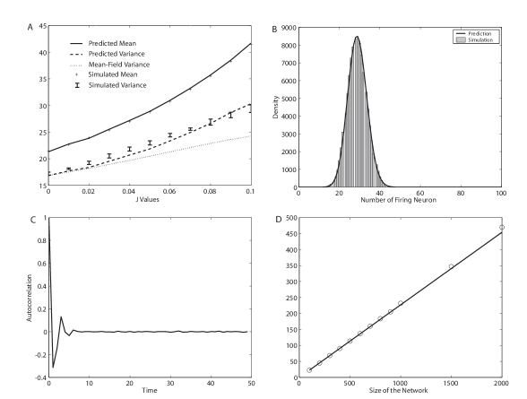
Figure 9: Conductance Synapse model – A) Mean (crosses) and variance (diamonds) versus $J$ from the numerical simulation compare well with the predictions (solid and dashed lines). Parameters are $N=100$, $I=4$, $\sigma=2.0$. B) The numerical PDF(histogram) and prediction (solid line) for $N=100$, $I=4$, $\sigma=2.0$, $J=0.05$. C) The autocorrelation (solid line) for a network of $N=1500$. The dashed line is the estimated exponential decay with $\lambda=Cov(1)/Var$ (see text). Parameters are $J=0.05$, $I=4$, $\sigma=2.0$ and $\lambda=0.31$. D) The variance (circles) versus $N$. The solid line is from equation (21) with $\lambda$ computed using the autocorrelation decay for $N=1500$ ($\lambda=0.31$) displayed in C). Parameters are $J=0.05$, $I=4$, $\sigma=2.0$.

for all $X\in\{0,...,N\}$ using the same method as in the current-based model. From the response function, we obtained the MTM and the invariant measure. Figure 9A compares the mean and variance of a numerical simulation with the Markov prediction for varying $J$. We see that there is a good match. For $J=0.05$, we compare the numerically computed PDF with the invariant measure. As shown in figure 9B, the prediction is extremely accurate. We estimated the slope factor as in the previous section using the autocorrelation function for $N=1500$ and found $\lambda=0.31$ and computed the estimated variance for various $N$. The comparison is shown on figure 9D. There is again a close match.

VI Discussion

Our model relies on the assumption that the neuronal dynamics can be represented by a Markov process. We partition time into discrete epochs and the probability that a neuron will fire in one epoch only depends on the activity of the previous epoch. For this approximation to be valid, at least two conditions must be met. The first is that the epoch time needs to be long enough so that the influence of activity in the distant past is negligible. The second is that the epoch time needs to be short enough so that a neuron fires at most once within an epoch. The influence time of a neuron is given approximately by the larger of the membrane time constant ($\tau_{m}$) and synaptic time constant ($\tau_{s}$). Presumably, the neuron does not have a memory of events much beyond this time scale. This gives a lower bound on the epoch time $\Delta t$. Hence, $\Delta t>\max[\tau_{m},\tau_{s}]$. The second condition is equivalent to $f\Delta t<1$, where $f$ is the max firing rate of a neuron in the network. Thus, the Markov model is applicable for

$$\max[\tau_{m},\tau_{s}]<f^{-1}$$ (49)

This condition is not too difficult to satisfy. For example, a cortical neuron receiving AMPA inputs with a membrane time constant less than 20 ms can satisfy the Markov condition if its maximum firing rate is below 50 Hz. Since typical cortical neurons have a membrane time constant between 1 and 20 ms and many recordings in the cortex find rates below 50 Hz Nicholls et al. (1992), our formalism could be applicable to a broad class of cortical circuits.

The equilibrium state of our Markov model exists and is exactly solvable if the response function is never zero or one. In other words, a neuron in the network always has a nonzero probability to fire but never has full certainty it will fire. Hence, the neuronal dynamics are always fully stochastic. Thus the equilibrium state of a fully stochastic network could be another definition of the asynchronous state. However, even though the network is completely stochastic, the activity is not uncorrelated. These correlations are manifested in the entire network activity but not within the firing statistics of the individual neurons, which obey a simple random binomial or Poisson distribution. The autocorrelation function of the individual neuron also decays much more quickly than that of the network.

Many previous approaches to studying the asynchronous state assumed that neuronal firing was statistically independent so a mean-field description was valid. With our simple model, we can compute the equilibrium PDF directly and explicitly determine the parameter regimes where mean-field theory breaks down. We also show that the “order parameter” that determines nearness to criticality is the slope of the response function around the equilibrium mean activity. As expected, we find that mean-field theory is less applicable for small or strongly recurrent neural circuits. In our model, the mean activity of our network can be obtained using mean-field theory except at the critical point. We compute the variance of the network activity directly and see precisely how the network dynamics deviate from mean-field theory as we approach the critical point. We note that while our closed-form estimates for the mean and variance may break down very near criticality, our model does not. The invariant measure of the MTM still gives the equilibrium PDF and in principle can be computed to arbitrary precision. Hence, our model can serve as a simple example of when mean-field theory is applicable. We note that even in the limit of $N$ going to infinity, the variance of the network deviates from a network of independent neurons by a factor of $(1-\lambda)^{-1}$. The deviations from mean-field theory persist even in an infinite sized network.

Our model requires statistical homogeneity. While purely homogeneous networks are unrealistic for biological networks, statistical homogeneity may be more plausible. For some classes of inputs, the probability of firing for a given set of neurons could be uniform over some limited temporal duration. We found that our analytical estimates can be modified to account for disordered randomness in the connections. A model that fully incorporated all heterogeneous effects would require taking into account different populations. However, with each additional population, the dimension of the MTM increases by a power of $N$. Thus for a network of two populations, say inhibitory and excitatory neurons, the resulting problem will involve a MTM with $N^{2}\times N^{2}$ elements.

Future work could examine the behavior at the critical point more carefully. Our variance estimate predicted that the variance at criticality would diverge as the system size squared but simulations found an exponent of 3/2. We also showed that the correlation time of the network activity diverged at the critical point. We expect correlations to obey a power law at criticality. Perhaps, a renormalization group approach may be adapted to study the scaling behavior near criticality. Recent experiments have found that cortical slices exhibit critical behavior Beggs and Plenz (2004, 2003). Our Markov model may be an ideal system to explore critical behavior.

Finally, we note that even at the critical point, where the network activity is highly correlated, the single neuron dynamics can exhibit uncorrelated Poisson statistics. This shows that collective network dynamics may not be deducible from single neuron dynamics. Using our model as a basis, it may be possible to probe characteristics about local network size, connectivity and nearness to criticality by combining recordings of single neurons with measurements of the local field potential.

VII Acknowledgments

This works was supported by the Intramural Research Program of NIH, NIDDK. We would like to thank Michael Buice for his helpful comments on the manuscript.

Appendix A Mean and variance derivations

The mean activity is given by

$$\langle X\rangle_{t} = \sum_{k=0}^{N}kP_{k}(t)$$

$$= \sum_{k=0}^{N}k\sum_{i=0}^{N}C_{N}^{k}(1-p_{i})^{N-k}p_{i}^{k}P_{i}(t-1)$$

Rearranging yields

$$\langle X\rangle_{t}=\sum_{i=0}^{N}P_{i}(t-1)\sum_{k=0}^{N}kC_{N}^{k}(1-p_{i})^{N-k}p_{i}^{k}$$

Since $\sum_{k=0}^{N}kC_{N}^{k}(1-p_{i})^{N-k}p_{i}^{k}=Np_{i}$ is the mean of a binomial distribution, we obtain

$$\langle X\rangle_{t} = \sum_{i=0}^{N}P_{i}(t-1)Np_{i}$$

$$= N\langle p\rangle_{t-1}$$

which is (8).

The variance is given by

$$Var_{t}(X) = \sum_{k=0}^{N}k^{2}P_{k}(t)-N^{2}\langle p\rangle_{t-1}^{2}$$

$$= \sum_{k=0}^{N}k^{2}\sum_{i=0}^{N}C_{N}^{k}(1-p_{i})^{N-k}p_{i}^{k}P_{i}(t-1)-N^{2}\langle p\rangle_{t-1}^{2}$$

$$= \sum_{i=0}^{N}P_{i}(t-1)\sum_{k=0}^{N}k^{2}C_{N}^{k}(1-p_{i})^{N-k}p_{i}^{k}-N^{2}\langle p\rangle_{t-1}^{2}$$

$$= \sum_{i=0}^{N}P_{i}(t-1)Np_{i}(1-p_{i})+\sum_{i=0}^{N}P_{i}(t-1)N^{2}p_{i}^{2}-N^{2}\langle p\rangle_{t-1}^{2}$$

$$= N\langle p(1-p)\rangle_{t-1}+N^{2}Var_{t-1}(p)$$

where we have used the variance of a binomial distribution $Np(1-p)$. For the linear case, writing $p(X)=a+bX$ we have

$$Var_{\mu}(X) = N\langle p(1-p)\rangle_{\mu}+N^{2}\langle p^{2}\rangle_{\mu}-N^{2}\langle p\rangle_{\mu}^{2}$$

$$= N\langle a+bX-a^{2}-2abX-b^{2}X^{2}\rangle_{\mu}+N^{2}\langle a^{2}+2abX+b^{2}X^{2}\rangle_{\mu}-N^{2}\langle a+bX\rangle_{\mu}^{2}$$

$$= Na+bN\langle X\rangle-Na^{2}-2Nab\langle X\rangle-Nb^{2}\langle X^{2}\rangle+N^{2}a^{2}+2N^{2}ab\langle X\rangle+N^{2}b^{2}\langle X^{2}\rangle$$

$$-N^{2}(a^{2}+2ab\langle X\rangle+b^{2}\langle X\rangle^{2})$$

$$= Na-Na^{2}+N^{2}a^{2}-N^{2}a^{2}+\langle X\rangle(bN-2Nab+2N^{2}ab-2N^{2}ab)$$

$$+\langle X^{2}\rangle(-Nb^{2}+N^{2}b^{2})-b^{2}N^{2}\langle X\rangle^{2}$$

$$= Na-Na^{2}+bN(1-2a)\langle X\rangle+(N^{2}b^{2}-Nb^{2})Var(X)-Nb^{2}\langle X\rangle^{2}$$

$$= \frac{Na-Na^{2}+bN(1-2a)\langle X\rangle-Nb^{2}\langle X\rangle^{2}}{1-N^{2}b^{2}+Nb^{2}}$$

Setting $a=p_{0}$ and $b=\frac{(q-p_{0})}{Nm}$ gives

$$Var_{\mu}(X)=q^{2}N\frac{p_{0}(1-p_{0})+(q-p_{0})(1-p_{0}-q)}{q^{2}-(q-p_{0})^{2}+(q-p_{0})^{2}/N}$$ (50)

If we set $\lambda=(q-p_{0})/q$ we get equation (21).

Appendix B Autocovariance function

We prove the form of the autocovariance function $Cov(\tau)=\lambda^{\tau}Var_{\mu}(X)$ for the linear response function using induction. We first show that $Cov(1)=\lambda Var_{\mu}(X)$ and then $Cov(\tau+1)=\lambda Cov(\tau)$.

The autocovariance function when $\tau=1$ is given by

$$\rm{Cov}(1) = \langle X_{t}X_{t+1}\rangle-\langle X\rangle^{2}_{\mu}$$

$$= \sum_{k=0}^{N}\sum_{i=0}^{N}kiP(X_{t+1}=i|X_{t}=k)P(X_{t}=k)-\langle X\rangle^{2}_{\mu}$$

$$= N\sum_{k=0}^{N}kp_{k}P(X_{t}=k)-\langle X\rangle^{2}_{\mu}$$

$$= N\langle pX\rangle_{\mu}-\langle X\rangle^{2}_{\mu}$$

For a linear response function $p$, we obtain

$$\rm{Cov}(1) = N\langle pX\rangle_{\mu}-\langle X\rangle^{2}_{\mu}$$

$$= N\langle p_{0}X+\frac{q-p_{0}}{Nq}X^{2}\rangle_{\mu}-N^{2}m^{2}$$

$$= N^{2}p_{0}q+\langle\frac{q-p_{0}}{q}X^{2}\rangle_{\mu}-N^{2}q^{2}$$

$$= N^{2}q\left(p_{0}-q\right)+\frac{q-p_{0}}{q}\left(Var_{\mu}(X)+N^{2}q^{2}\right)$$

$$= \frac{q-p_{0}}{q}Var_{\mu}(X)$$

Hence for $\tau=1$, the autocovariance function is equal to the slope factor $\lambda=(q-p_{0})/q$ times the variance. Assume for $\tau$, that $Cov(\tau)=\lambda^{\tau}Var_{\mu}(X)$, then

$$Cov(\tau+1) = \langle X_{t}X_{t+\tau+1}\rangle-\langle X\rangle^{2}_{\mu}$$

$$= \sum_{k=0}^{N}\sum_{j=0}^{N}kjP(X_{t}=k)P(X_{t+\tau+1}=j|X_{t}=k)-\langle X\rangle^{2}_{\mu}$$

$$= \sum_{k=0}^{N}\sum_{j=0}^{N}kjP(X_{t}=k)\sum_{r=0}^{N}P(X_{t+\tau+1}=j|X_{t+\tau}=r)P(X_{t+\tau}=r|X_{t}=k)-\langle X\rangle^{2}_{\mu}$$

$$= \sum_{k=0}^{N}\sum_{j=0}^{N}\sum_{r=0}^{N}kjP(X_{t}=k)C_{N}^{j}(1-p(r))^{N-j}p(r)^{j}P(X_{t+\tau}=r|X_{t}=k)-\langle X\rangle^{2}_{\mu}$$

$$= \sum_{k=0}^{N}\sum_{r=0}^{N}Nkp(r)P(X_{t}=k)P(X_{t+\tau}=r|X_{t}=k)-\langle X\rangle^{2}_{\mu}$$

using the mean of the binomial distribution. We can now insert the linear response function to obtain

$$Cov(\tau+1) = \sum_{k=0}^{N}\sum_{r=0}^{N}Nk(p_{0}+\frac{q-p_{0}}{Nq}r)P(X_{t}=k)P(X_{t+\tau}=r|X_{t}=k)-\langle X\rangle^{2}_{\mu}$$

$$= \sum_{k=0}^{N}\sum_{r=0}^{N}Nkp_{0}P(X_{t}=k)P(X_{t+\tau}=r|X_{t}=k)+\frac{q-p_{0}}{q}\left(Cov(\tau)+\langle X\rangle^{2}_{\mu}\right)-\langle X\rangle^{2}_{\mu}$$

because

$$\sum_{k=0}^{N}\sum_{r=0}^{N}krP(X_{t}=k)P(X_{t+\tau}=r|X_{t}=k)=Cov(t+\tau)+\langle X\rangle^{2}_{\mu}$$

Then since

$$\sum_{k=0}^{N}\sum_{r=0}^{N}Nkp_{0}P(X_{t}=k)P(X_{t+\tau}=r|X_{t}=k)=\sum_{k=0}^{N}Nkp_{0}P(X_{t}=k)$$

because

$$\sum_{r=0}^{N}P(X_{t+\tau}=r|X_{t}=k)=1$$

for all $k$ and

$$\sum_{k=0}^{N}Nkp_{0}P(X_{t}=k)=\langle Np_{0}X\rangle_{\mu}=N^{2}p_{0}q$$

we finally obtain

$$Cov(\tau+1) = N^{2}p_{0}q+\frac{q-p_{0}}{q}\langle X\rangle^{2}_{\mu}-\langle X\rangle^{2}_{\mu}+\lambda Cov(\tau)$$

$$= N^{2}p_{0}q+\frac{q-p_{0}}{q}N^{2}q^{2}-N^{2}q^{2}+\lambda Cov(\tau)$$

$$= N^{2}(p_{0}q+(q-p_{0})q-q^{2})+\lambda Cov(\tau)$$

$$= \lambda Cov(\tau)$$

proving equation (24) by induction.

Figures

References

- Singer and Gray (1995) W. Singer and C. M. Gray, Annu Rev Neurosci 18, 555 (1995).
- Fries et al. (2001) P. Fries, J. H. Reynolds, A. E. Rorie, and R. Desimone, Science 291, 1560 (2001).
- Pesaran et al. (2002) B. Pesaran, J. S. Pezaris, M. Sahani, P. P. Mitra, and R. A. Andersen, Nat Neurosci 5, 805 (2002).
- Steinmetz et al. (2000) P. N. Steinmetz, A. Roy, P. J. Fitzgerald, S. S. Hsiao, K. O. Johnson, and E. Niebur, Nature 404, 187 (2000).
- Softky and Koch (1993) W. R. Softky and C. Koch, J Neurosci 13, 334 (1993).
- Amit and Brunel (1997a) D. J. Amit and N. Brunel, Network: Comput. Neural. Syst. 8, 373 (1997a).
- Amit and Brunel (1997b) D. J. Amit and N. Brunel, Cereb Cortex 7, 237 (1997b).
- Van Vreeswijk and Sompolinsky (1996) C. Van Vreeswijk and H. Sompolinsky, Science 274, 1724 (1996).
- Van Vreeswijk and Sompolinsky (1998) C. Van Vreeswijk and H. Sompolinsky, Neural Comput 10, 1321 (1998).
- Gerstner (2000) W. Gerstner, Neural Computation 12, 43 (2000).
- Cai et al. (2004) D. Cai, L. Tao, M. Shelley, and D. W. McLaughlin, Proc Natl Acad Sci U S A 101, 7757 (2004).
- Gerstner and Kistler (2002a) W. Gerstner and W. Kistler, Spiking Neuron Models - Single Neurons, Populations, Plasticity (Cambrige University Press, Cambridge, UK, 2002a).
- Abbott and Vreeswijk (1993) L. Abbott and C. Vreeswijk, Phys. Rev. E 48, 1483 (1993).
- Treves (1993) A. Treves, Network 4, 259 (1993).
- Fusi and Mattia (1999) S. Fusi and M. Mattia, Neural Computation 11, 633 (1999).
- Golomb and Hansel (2000) D. Golomb and D. Hansel, Neural Comput 12, 1095 (2000).
- Brunel (2000a) N. Brunel, J Comput Neurosci 8, 183 (2000a).
- Nykamp and Tranchina (2000) D. Nykamp and D. Tranchina, Journal of Computational Neuroscience 8, 19 (2000).
- Hansel and Mato (2003) D. Hansel and G. Mato, Neural Comput 15, 1 (2003).
- Del Giudice and Mattia (2003) P. Del Giudice and M. Mattia, in Advances in Condensed Matter and Statistical Physics (Nova Science, Hauppauge, NY, 2003), pp. 125–153.
- Brunel and Hansel (2006) N. Brunel and D. Hansel, Neural Comput 18, 1066 (2006).
- Plesser and Gerstner (2000) H. E. Plesser and W. Gerstner, Neural Computation 12, 367 (2000).
- Salinas and Sejnowski (2002) E. Salinas and T. J. Sejnowski, Neural Comput 14, 2111 (2002).
- Fourcaud and Brunel (2002) N. Fourcaud and N. Brunel, Neural Comput 14, 2057 (2002).
- Soula et al. (2006) H. Soula, G. Beslon, and O. Mazet, Neural Computation 18, 60 (2006).
- Ginzburg and Sompolinsky (1994) I. Ginzburg and H. Sompolinsky, Phys Rev E Stat Nonlin Soft Matter Phys 50, 3171 (1994).
- Meyer and Van Vreeswijk (2002) C. Meyer and C. Van Vreeswijk, Neural Computation 14, 369 (2002).
- Brunel (2003b) N. Brunel, Cereb Cortex 13, 1151 (2003b).
- Mattia and del Giudice (2002) M. Mattia and P. del Giudice, Physical Review E 66 (2002).
- Gerstner and Hemmen (1992) W. Gerstner and J. v. Hemmen, Network 3, 139 (1992).
- Gerstner (1995) W. Gerstner, Physical Review. E. Statistical Physics, Plasmas, Fluids, and Related Interdisciplinary Topics 51, 738 (1995).
- Seung (1996) H. S. Seung, Proc Natl Acad Sci U S A 93, 13339 (1996).
- Kuznetsov (1998) Y. Kuznetsov, Elements of Bifurcation Theory 2nd ed. (Springer, 1998).
- Compte et al. (2000) A. Compte, N. Brunel, P. S. Goldman-Rakic, and X. J. Wang, Cereb Cortex 10, 910 (2000).
- Laing and Chow (2001) C. R. Laing and C. C. Chow, Neural Comput 13, 1473 (2001).
- Gutkin et al. (2001) B. S. Gutkin, C. R. Laing, C. L. Colby, C. C. Chow, and G. B. Ermentrout, J Comput Neurosci 11, 121 (2001).
- Compte (2006) A. Compte, Neuroscience 139, 135 (2006).
- Risken (1989) H. Risken, The Fokker-Planck Equation: Methods of Solution and Application 2nd ed (Springer, 1989).
- Hopfield (1982) J. Hopfield, Proc. Natl. Acad. Sci. USA 79, 2554 (1982).
- Nicholls et al. (1992) J. Nicholls, A. Martin, and B. Wallace, From Neuron To Brain Third Ed. (Sinauer Associates, Inc, Sunderland, MA, 1992).
- Beggs and Plenz (2004) J. M. Beggs and D. Plenz, J Neurosci 24, 5216 (2004).
- Beggs and Plenz (2003) J. M. Beggs and D. Plenz, J Neurosci 23, 11167 (2003).