Oscillations in I/O Monotone Systems
under Negative Feedback

Abstract

Oscillatory behavior is a key property of many biological systems. The Small-Gain Theorem (SGT) for input/output monotone systems provides a sufficient condition for global asymptotic stability of an equilibrium and hence its violation is a necessary condition for the existence of periodic solutions. One advantage of the use of the monotone SGT technique is its robustness with respect to all perturbations that preserve monotonicity and stability properties of a very low-dimensional (in many interesting examples, just one-dimensional) model reduction. This robustness makes the technique useful in the analysis of molecular biological models in which there is large uncertainty regarding the values of kinetic and other parameters. However, verifying the conditions needed in order to apply the SGT is not always easy. This paper provides an approach to the verification of the needed properties, and illustrates the approach through an application to a classical model of circadian oscillations, as a nontrivial “case study,” and also provides a theorem in the converse direction of predicting oscillations when the SGT conditions fail.

Keywords:.  Circadian rhythms, monotone systems, negative feedback, periodic behaviors

1 Introduction

Motivated by applications to cell signaling, our previous paper [1] introduced the class of monotone input/output systems, and provided a technique for the analysis of negative feedback loops around such systems. The main theorem gave a simple graphical test which may be interpreted as a monotone small gain theorem (“SGT” from now on) for establishing the global asymptotic stability of a unique equilibrium, a stability that persists even under arbitrary transmission delays in the feedback loop. Since that paper, various papers have followed-up on these ideas, see for example [26, 17, 16, 5, 11, 7, 10, 12, 4, 13, 34]. The present paper, which was presented in preliminary form at the 2004 IEEE Conference on Decision and Control, has two purposes.

The first purpose is to develop explicit conditions so as to make it easier to apply the SGT theorem, for a class of systems of biological significance, a subset of the class of tridiagonal systems with inputs and outputs. Tridiagonal systems (with no inputs and outputs) were introduced largely for the study of gene networks and population models, and many results are known for them, see for instance [31, 33]. Deep achievements of the theory include the generalization of the Poincaré-Bendixson Theorem, from planar systems to tridiagonal systems of arbitrary dimension, due to Mallet-Paret and Smith [28] as well as a later generalization to include delays due to Mallet-Paret and Sell [27]. For our class of systems, we provide in Theorem 1 sufficient conditions that guarantee the existence of characteristics (“nonlinear DC gain”), which is one of the ingredients needed in the SGT Theorem from [1].

Negative feedback is often associated with oscillations, and in that context one may alternatively view the failure of the SGT condition as providing a necessary condition for a system to exhibit periodic behaviors, and this is the way in which the SGT theorem has been often applied.

The conditions given in Theorem 1 arose from our analysis of a classical model of circadian oscillations. The molecular biology underlying the circadian rhythm in Drosophila is currently the focus of a large amount of both experimental and theoretical work. The most classical model is that of Goldbeter, who proposed a simple model for circadian oscillations in Drosophila, see [14] and the book [15]. The key to the Goldbeter model is the auto-inhibition of the transcription of the gene per. This inhibition is through a loop that involves translational and post-transcriptional modifications as well as nuclear translocation. Although, by now, several more realistic models are available, in particular incorporating other genes, see e.g. [24, 25], this simpler model exhibits many realistic features, such as a close to 24-hour period, and has been one of the main paradigms in the study of oscillations in gene networks. Thus, we use Goldbeter’s original model as our “case study” to illustrate the mathematical techniques.

The second purpose of this paper is to further explore the idea that, conversely, failure of the SGT conditions may lead to oscillations if there is a delay in the feedback loop. (As with the Classical Small Gain Theorem, of course the SGT is far from necessary for stability, unless phase is also considered.) As argued in [3], Section 3, and reviewed below, failure of the conditions often means that a “pseudo-oscillation” exists in the system (provided that delays in the feedback loop are large enough), in the rough sense that there are trajectories that “look” oscillatory if observed under very noisy conditions and for finite time-intervals. This begs the more interesting question of whether true periodic solutions exist. It turns out that some analogs of this converse result are known, for certain low-dimensional systems, see [29, 22]. In the context of failure of the SGT, Enciso recently provided a converse theorem for a class of cyclic systems, see [9]. The Goldbeter model is far from being cyclic, however. Theorem 2 in this paper proves the existence of oscillations for a class of monotone tridiagonal systems under delayed negative feedback, and the theorem is then illustrated with the Goldbeter circadian model.

We first review the basic setup from [1].

2 I/O Monotone Systems, Characteristics, and Negative Feedback

We consider an input/output system

$$\frac{dx}{dt}=f(x,u),\;\;y=h(x)\,,$$ (1)

in which states $x(t)$ evolve on some subset $X\subseteq{\mathbb{R}}^{n}$, and input and output values $u(t)$ and $y(t)$ belong to subsets $U\subseteq{\mathbb{R}}^{m}$ and $Y\subseteq{\mathbb{R}}^{p}$ respectively. The maps $f:X\times U\rightarrow{\mathbb{R}}^{n}$ and $h:X\rightarrow Y$ are taken to be continuously differentiable. An input is a signal $u:[0,\infty)\rightarrow U$ which is locally essentially compact (meaning that images of restrictions to finite intervals are compact), and we write $\varphi(t,x_{0},u)$ for the solution of the initial value problem $dx/dt(t)=f(x(t),u(t))$ with $x(0)=x_{0}$, or just $x(t)$ if $x_{0}$ and $u$ are clear from the context, and $y(t)=h(x(t))$. Given three partial orders on $X,U,Y$ (we use the same symbol $\prec$ for all three orders), a monotone input/output system (“MIOS”), with respect to these partial orders, is a system (1) which is forward-complete (for each input, solutions do not blow-up on finite time, so $x(t)$ and $y(t)$ are defined for all $t\geq 0$), $h$ is a monotone map (it preserves order) and: for all initial states $x_{1},x_{2}$ for all inputs $u_{1},u_{2}$, the following property holds: if $x_{1}$$\preceq$$x_{2}$ and $u_{1}$$\preceq$$u_{2}$ (meaning that $u_{1}(t)$$\preceq$$u_{2}(t)$ for all $t$$\geq$$0$), then $\varphi(t,x_{1},u)$$\preceq$$\varphi(t,x_{2},u_{2})$ for all $t>0$. Here we consider partial orders induced by closed proper cones $K\subseteq{\mathbb{R}}^{\ell}$, in the sense that $x\preceq y$ iff $y-x\in K$. The cones $K$ are assumed to have a nonempty interior and are pointed, i.e. $K\bigcap-K=\{0\}$. When there are no inputs nor outputs, the definition of monotone systems reduces to the classical one of monotone dynamical systems studied by Hirsch, Smith, and others [32], which have especially nice dynamics. Not only is chaotic or other irregular behavior ruled out, but, in fact, under additional technical conditions (strong monotonicity) almost all bounded trajectories converge to the set of steady states (Hirsch’s generic convergence theorem [19, 20]).

The most interesting particular case is that in which $K$ is an orthant cone in ${\mathbb{R}}^{n}$, i.e. a set $S_{\varepsilon}$ of the form $\{x\in{\mathbb{R}}^{n}\,|\,\varepsilon_{i}x_{i}\geq 0\}$, where $\varepsilon_{i}=\pm 1$ for each $i$. A useful test for monotonicity with respect to arbitrary orthant cones (“Kamke’s condition” in the case of systems with no inputs and outputs) is as follows. Let us assume that all the partial derivatives $\frac{\partial f_{i}}{\partial x_{j}}(x,u)$ for $i\not=j$, $\frac{\partial f_{i}}{\partial u_{j}}(x,u)$ for all $i,j$, and $\frac{\partial h_{i}}{\partial x_{j}}(x)$ for all $i,j$ (subscripts indicate components) do not change sign, i.e., they are either always $\geq 0$ or always $\leq 0$. We also assume that $X$ is convex (much less is needed.) We then associate a directed graph $G$ to the given MIOS, with $n+m+p$ nodes, and edges labeled “$+$” or “$-$” (or $\pm 1$), whose labels are determined by the signs of the appropriate partial derivatives (ignoring diagonal elements of $\partial f/\partial x$). One may define in an obvious manner undirected loops in $G$, and the parity of a loop is defined by multiplication of signs along the loop. (See e.g. [2] for more details.) A system is monotone with respect to some orthant cones in $X,U,Y$ if and only if there are no negative loops in $G$. In particular, if the cone is the main orthant ($\varepsilon=(1,\ldots,1)$), the requirement is that all partial derivatives must be nonnegative, with the possible exception of the diagonal terms of the Jacobian of $f$ with respect to $x$. A monotone system with respect to the main orthant is also called a cooperative system. This condition can be extended to non-orthant cones, see [30, 35, 36, 37].

In order to define negative feedback (“inhibitory feedback” in biology) interconnections we will say that a system is anti-monotone (with respect to given orders on input and output value spaces) if the conditions for monotonicity are satisfied, except that the output map reverses order: $x_{1}\preceq x_{2}\Rightarrow h(x_{2})\preceq h(x_{1})$.

2.1 Characteristics

A useful technical condition that simplifies statements (one may weaken the condition, see [26]) is that of existence of single-valued characteristics, which one may also think of as step-input steady-state responses or (nonlinear) DC gains. To define characteristics, we consider the effect of a constant input $u(t)\equiv u_{0}$, $t\geq 0$ and study the dynamical system $dx/dt=f(x,u_{0})$. We say that a single-valued characteristic exists if for each $u_{0}$ there is a state $K(u_{0})$ so that the system is globally attracted to $K(u_{0})$, and in that case we define the characteristic $k:U\rightarrow Y$ as the composition $h\circ K$. It is remarkable fact for monotone systems that (under weak assumptions on $X$, and boundedness of solutions) just knowing that a unique steady state $K(u_{0})$ exists, for a given input value $u_{0}$, already implies that $K(u_{0})$ is in fact a globally asymptotically stable state for $dx/dt=f(x,u_{0})$, see [23, 6].

2.2 Negative feedback

Monotone systems with well-defined characteristics constitute useful building blocks for arbitrary systems, and they behave in many senses like one-dimensional systems. Cascades of such systems inherit the same properties (monotone, monostable response). Under negative feedback, one obtains non-monotone systems, but such feedback loops sometimes may be profitably analyzed using MIOS tools.

We consider a feedback interconnection of a monotone and an anti-monotone input/output system:

$$\frac{dx_{1}}{dt} = f_{1}(x_{1},u_{1}),\;\;y_{1}=h_{1}(x_{1})$$ (2)

$$\frac{dx_{2}}{dt} = f_{2}(x_{2},u_{2}),\;\;y_{2}=h_{2}(x_{2})$$ (3)

with characteristics denoted by “$k$” and “$g$” respectively. (We can also include the case when the second system is a static function $y_{2}(t)=g(u_{2}(t))$.) As in [2], we will require here that the inputs and outputs of both systems are scalar: $m_{1}$$=$$m_{2}$$=$$p_{1}$$=$$p_{2}$$=1$; the general case [8] is similar but requires more notation and is harder to interpret graphically. The feedback interconnection of the systems (2) and (3) is obtained by letting $u_{2}$$=$$y_{1}$$=$“$y$” and $u_{1}$$=$$y_{2}$$=$“$u$”, as depicted (assuming the usual real-number orders on inputs and outputs) in Figure 1.

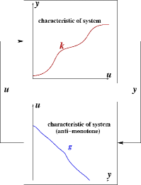
Figure 1: Negative feedback configuration

The main result from [1], which we’ll refer to as the monotone SGT theorem, is as follows. We plot together $k$ and $g^{-1}$, as shown in Figure 2,

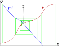
Figure 2: characteristics

and consider the following discrete dynamical system:

$$u^{+}=(g\circ k)(u)$$

on $U$. Then, provided that solutions of the closed-loop system are bounded, the result is that, if this iteration has a globally attractive fixed point ${\bar{u}}$, as shown in Figure 2 through a “spiderweb” diagram, then the feedback system has a globally attracting steady state. (An equivalent condition, see Lemma 2.3 in [7], and [11], is that the discrete system should have no nontrivial period-two orbits, i.e. the equation $(g\circ k)(u)=u$ has a unique solution.)

It is not hard to prove, furthermore, that arbitrary delays may be allowed in the feedback loop. In other words, the feedback could be of the form $u(t)=y(t-h)$, and such delays (even with $h=h(t)$ time varying or even state-dependent, as long as $t-h(t)\rightarrow\infty$ as $t\rightarrow\infty$) do not destroy global stability of the closed loop. Moreover, it is also known [10] that diffusion does not destroy global stability: a reaction-diffusion system, with Neumann boundary conditions, whose reaction can be modeled in the shown feedback configuration, has the property that all solutions converge to a (unique) uniform in space solution.

2.3 Robustness

It is important to point out that characteristics (called dose response curves, activity plots, steady-state expression of a gene in response to an external ligand, etc.) are frequently readily available from experimental data, especially in molecular biology and pharmacology, in contrast to the rare availability and high uncertainty regarding the precise form of the differential equations defining the dynamics and values for all parameters (kinetic constants, for example) appearing in the equations. MIOS analysis allows one to combine the numerical information provided by characteristics with the qualitative information given by “signed network topology” (Kamke condition) in order to predict global behavior. (See [34] for a longer discussion of this “qualitative-quantitative approach” to systems biology.) The conclusions from applying the monotone SGT are robust with respect to all perturbations that preserve monotonicity and stability properties of the 1-d iteration.

Moreover, even if one would have a complete system specification, the 1-d iteration plays a role vaguely analogous to that of Nyquist plots in classical control design, where the use of a simple plot allows quick conclusions that would harder to obtain, and be far less intuitive, when looking at the entire high-dimensional system.

3 Existence of Characteristics

The following result is useful when showing that characteristics exist for some systems of biological interest, including the protein part of the circadian model described later. The constant $c$ represents the value of a constant control $u(t)\equiv c$.

Theorem 1

Consider a system of the following form:

$$\dot{x}_{0} = c-\alpha_{0}(x_{0})+\beta_{0}(x_{1})$$

$$\vdots$$

$$\dot{x}_{i} = \alpha_{i-1}(x_{i-1})-\beta_{i-1}(x_{i})-\alpha_{i}(x_{i})+\beta_{i}(x_{i+1})$$

$$\quad\quad\quad\quad i=1,\ldots,n-2$$

$$\vdots$$

$$\dot{x}_{n-1} = \alpha_{n-2}(x_{n-2})-\beta_{n-2}(x_{n-1})-\alpha_{n-1}(x_{n-1})$$

$$\quad\quad\quad\quad+\beta_{n-1}(x_{n})-\theta(x_{n-1})$$

$$\dot{x}_{n} = \alpha_{n-1}(x_{n-1})-\beta_{n-1}(x_{n})$$

evolving on ${\mathbb{R}}_{\geq 0}^{n+1}$, where $c\geq 0$ is a constant. Assume that $\theta$ and all the $\alpha_{i},\beta_{i}$ are differentiable functions $[0,\infty)\rightarrow[0,\infty)$ with everywhere positive derivatives and vanishing at $0$,

$$\theta\;\;\mbox{and}\;\;\alpha_{i},\beta_{i},\,i=0,\ldots,n-2\;\;\mbox{are bounded,}$$

and

$$\alpha_{n-1},\beta_{n-1}\;\;\mbox{are unbounded}.$$

We use the notation $\theta(\infty)$ to indicate $\lim_{r\rightarrow\infty}\theta(r)$, and similarly for the other bounded functions. Furthermore, suppose that the following conditions hold:

$$\alpha_{i-1}(\infty)+\beta_{i}(\infty)<\alpha_{i}(\infty)+\beta_{i-1}(\infty)\,\;\;i=1,\ldots,n-2$$ (4)

$$\theta(\infty)+\beta_{i}(\infty)<\alpha_{i}(\infty),\;\;i=0,\ldots,n-2$$ (5)

$$c<\theta(\infty).$$ (6)

Then, there is a (unique) globally asymptotically stable equilibrium for the system.

Observe that (5) (applied with $i=0$) together with (6) imply that also:

$$c+\beta_{0}(\infty)<\alpha_{0}(\infty)\,.$$ (7)

Proof. We start by noticing that solutions are defined for all $t\geq 0$. Indeed, consider any maximal solution $x(t)=(x_{0}(t),x_{1}(t),\ldots,x_{n}(t))$. From

$$\frac{d}{dt}\left(x_{0}+x_{1}+\ldots+x_{n}\right)\;=\;c-\theta(x_{n-1})\;\leq\;c\,,$$ (8)

we conclude that there is an estimate $x_{i}(t)\leq\sum_{i}x_{i}(t)\leq\sum_{i}x_{i}(0)+tc$ for each coordinate of $x$, and hence that there are no finite escape times.

Moreover, we claim that $x(\cdot)$ is bounded. We first show that $x_{0},\ldots,x_{n-2}$ are bounded. For $x_{0}$, it is enough to notice that $\dot{x}_{0}\leq c-\alpha_{0}(x_{0})+\beta_{0}(\infty)$, so that

$$x_{0}(t)>\alpha_{0}^{-1}(c+\beta_{0}(\infty))\;\;\Rightarrow\;\;\dot{x}_{0}(t)<0$$

so (7) shows that $x_{0}$ is bounded. Similarly, for $x_{i}$, $i=1,\ldots,n-2$ we have that

$$\dot{x}_{i}\leq\alpha_{i-1}(\infty)-\beta_{i-1}(x_{i})-\alpha_{i}(x_{i})+\beta_{i}(\infty)$$

so (4) provides boundedness of these coordinates as well.

Next we show boundedness of $x_{n-1}$ and $x_{n}$.

Since the system is a strongly monotone tridiagonal system, we know (see [31], Corollary 1), that $x_{n}(t)$ is eventually monotone. That is, for some $T>0$, either

$$\dot{x}_{n}(t)\geq 0\;\;\;\forall\,t\geq T$$ (9)

or

$$\dot{x}_{n}(t)\leq 0\;\;\;\forall\,t\geq T\,.$$ (10)

Hence, $x_{n}(t)$ admits a limit, either finite or infinite.

Assume first that $x_{n}$ is unbounded, which means that $x_{n}(t)\rightarrow\infty$ because of eventual monotonicity. Then, case (10) cannot hold, so (9) holds. Therefore,

$$\alpha_{n-1}(x_{n-1}(t))-\beta_{n-1}(x_{n}(t))\;=\;\dot{x}_{n}\;\geq\;0$$

for all $t\geq T$, which implies that

$$x_{n-1}(t)\;\geq\;\alpha_{n-1}^{-1}(\beta_{n-1}(x_{n}(t)))\rightarrow\infty$$

as well. Looking again at (8), and using that $c-\theta(\infty)<0$ (property (6)), we conclude that

$$\frac{d}{dt}\left(x_{0}+x_{1}+\ldots+x_{n-1}+x_{n}\right)(t)\;<\;0$$

for all $t$ sufficiently large. Thus $x_{0}+x_{1}+\ldots+x_{n-1}+x_{n}$ is bounded (and nonnegative), and this implies that $x_{n-1}$ is bounded, a contradiction since we showed that $x_{n-1}\rightarrow\infty$. So $x_{n}$ is bounded.

Next, notice that $\dot{x}_{n-1}\leq\alpha_{n-2}(x_{n-2})+\beta_{n-1}(x_{n})-\alpha_{n-1}(x_{n-1})$. The two positive terms are bounded, because both $x_{n-2}$ and $x_{n}$ are bounded. Thus,

$$\dot{x}_{n-1}\leq v(t)-\alpha_{n-1}(x_{n-1})\,,$$

where $0\leq v(t)\leq k$ for some constant $k$. Thus $\dot{x}_{n-1}(t)<0$ whenever $x_{n-1}(t)>\alpha_{n-1}^{-1}(k)$, and this proves that $x_{n-1}$ is bounded, as claimed.

Once that boundedness has been established, if we also show that there is a unique equilibrium, then the theory of strongly monotone tridiagonal systems ([31, 32]) (or [23, 6] for more general monotone systems results) will ensure global asymptotic stability of the equilibrium. So we show that equilibria exist and are unique.

Let us write $f_{i}(x)$ for the right-hand sides of the equations, so that $\dot{x}_{i}=f_{i}(x)$ for each $i$. We need to show that there is a unique nonnegative solution $x=(x_{0},\ldots,x_{n})$ of

$$f_{0}(x)=\ldots=f_{n}(x)=0.$$

Equivalently, we can write the equations like this:

$$f_{n}(x) = 0$$

$$\vdots$$

$$f_{i}(x)+\ldots+f_{n}(x) = 0$$

$$\vdots$$

$$f_{0}(x)+f_{1}(x)\ldots+f_{n}(x) = 0$$ (13)

Since $f_{0}(x)+f_{1}(x)\ldots+f_{n}(x)=c-\theta(x_{n-1})$, (13) has the unique solution $x_{n-1}=\bar{x}_{n-1}=\theta^{-1}(c)$ which is well-defined because property (6) says that $c<\theta(\infty)$.

Next, we consider equation (3). This equation has the unique solution:

$$x_{n}\;=\;\bar{x}_{n}\;=\;\beta_{n-1}^{-1}(\alpha_{n-1}(\bar{x}_{n-1}))$$

which is well-defined because $\beta_{n-1}$ is a bijection.

Pick $i\in\{1,\ldots,n-1\}$ and suppose that we have uniquely determined $x_{j}=\bar{x}_{j}$ for each $j\geq i$. We will show that $x_{i-1}$ is also uniquely defined. Equation (3) is:

$$\alpha_{i-1}(x_{i-1})-\beta_{i-1}(\bar{x}_{i})-\theta(\bar{x}_{n-1})\;=\;0$$

and has the unique solution

$$x_{i-1}\;=\;\bar{x}_{i-1}\;=\;\alpha_{i-1}^{-1}(\beta_{i-1}(\bar{x}_{i})+\theta(\bar{x}_{n-1}))$$

which is well-defined because property (5) says that $\theta(\infty)+\beta_{i-1}(\infty)<\alpha_{i-1}(\infty)$ for each $i=1,\ldots,n-1$. By induction on $i=n-1,\ldots,1$, we have completed the uniqueness proof.  

4 The Goldbeter Circadian Model

The original Goldbeter model of Drosophila circadian rhythms is schematically shown in Figure 3.

Figure 3: Goldbeter’s Model

The assumption is that PER protein is synthesized at a rate proportional to its mRNA concentration. Two phosphorylation sites are available, and constitutive phosphorylation and dephosphorylation occur with saturation dynamics, at maximum rates $v_{i}$ and with Michaelis constants $K_{i}$. Doubly phosphorylated PER is degraded, also described by saturation dynamics (with parameters $v_{d},k_{d}$), and it is translocated to the nucleus, with rate constant $k_{1}$. Nuclear PER inhibits transcription of the per gene, with a Hill-type reaction of cooperativity degree $n$ and threshold constant $K_{I}$. The resulting mRNA is produced. and translocated to the cytoplasm, at a rate determined by a constant $v_{s}$. Additionally, there is saturated degradation of mRNA (constants $v_{m}$ and $k_{m}$).

Corresponding to these assumptions, and assuming a well-mixed system, one obtains an ODE system for concentrations are as follows:

$$\dot{M} = \frac{v_{s}K_{I}^{n}}{K_{I}^{n}+P_{N}^{n}}-\frac{v_{m}M}{k_{m}+M}$$

$$\dot{P}_{0} = k_{s}M-\frac{V_{1}P_{0}}{K_{1}+P_{0}}+\frac{V_{2}P_{1}}{K_{2}+P_{1}}$$

$$\dot{P}_{1} = \frac{V_{1}P_{0}}{K_{1}+P_{0}}-\frac{V_{2}P_{1}}{K_{2}+P_{1}}-\frac{V_{3}P_{1}}{K_{3}+P_{1}}+\frac{V_{4}P_{2}}{K_{4}+P_{2}}$$ (14)

$$\dot{P}_{2} = \frac{V_{3}P_{1}}{K_{3}+P_{1}}-\frac{V_{4}P_{2}}{K_{4}+P_{2}}-k_{1}P_{2}+k_{2}P_{N}-\frac{v_{d}P_{2}}{k_{d}+P_{2}}$$

$$\dot{P}_{N} = k_{1}P_{2}-k_{2}P_{N}$$

where the subscript $i=0,1,2$ in the concentration $P_{i}$ indicates the degree of phosphorylation of PER protein, $P_{N}$ is used to indicate the concentration of PER in the nucleus, and $M$ indicates the concentration of per mRNA.

The parameters (in suitable units $\mu M$ or $h^{-1}$) used by Goldbeter are given in Table 1.

Parameter	Value	Parameter	Value
$k_{2}$	1.3	$k_{1}$	1.9
$V_{1}$	3.2	$V_{2}$	1.58
$V_{3}$	5	$V_{4}$	2.5
$v_{s}$	0.76	$k_{m}$	0.5
$k_{s}$	0.38	$v_{d}$	0.95
$k_{d}$	0.2	$n$	4
$K_{1}$	2	$K_{2}$	2
$K_{3}$	2	$K_{4}$	2
$K_{I}$	1	$v_{m}$	0.65

Table 1: Parameter Values

With these parameters, there are limit cycle oscillations. If we take $v_{s}$ as a bifurcation parameter, a Hopf bifurcation occurs at $v_{s}\approx 0.638$.

As an illustration of the SGT, we will show now that the theorem applies when $v_{s}=0.4$. This means that not only will stability of an equilibrium hold globally in that case, but this stability will persist even if one introduces delays to model the transcription or translation processes. (Without loss of generality, we may lump these delays into one delay, say in the term $P_{N}$ appearing in the equation for $M$.) On the other hand, we’ll see later that the SGT discrete iteration does not converge, and in fact has a period-two oscillation, when $v_{s}=0.5$. This suggests that periodic orbits exist in that case, at least if sufficiently large delays are present, and we analyze the existence of such oscillations.

For the theoretical developments, we assume from now on that

$$v_{s}\leq 0.54$$ (15)

and the remaining parameters will be constrained below, in such a manner that those in the previously given table will satisfy all the constraints.

4.1 Breaking-up the Circadian System and Applying the SGT

We choose to view the system as the feedback interconnection of two subsystems, one for $M$ and the other one for $P$, see Figure 4.

Figure 4: Systems in feedback

mRNA Subsystem

The mRNA ($M$) subsystem is described by the scalar differential equation

$$\dot{M}\;=\;\frac{v_{s}K_{I}^{n}}{K_{I}^{n}+u_{1}^{n}}-\frac{v_{m}M}{k_{m}+M}$$

with input $u_{1}$ and output $y_{1}=k_{s}M$.

As state-space, we will pick a compact interval $X_{1}=[0,\bar{M}]$, where

$$\frac{v_{s}k_{m}}{v_{m}-v_{s}}\leq\bar{M}<\frac{v_{d}}{k_{s}}$$ (16)

and we assume that $v_{s}<v_{m}$. The order on $X_{1}$ is taken to be the usual order from ${\mathbb{R}}$.

Note that the first inequality implies that

$$v_{s}<\frac{v_{m}{\bar{M}}}{k_{m}+{\bar{M}}}$$ (17)

and therefore

$$\frac{v_{s}K_{I}^{n}}{K_{I}^{n}+u_{1}^{n}}-\frac{v_{m}{\bar{M}}}{k_{m}+{\bar{M}}}<0$$

for all $u_{1}\geq 0$, so that indeed $X_{1}$ is forward-invariant for the dynamics.

With the parameters shown in the table given earlier (except for $v_{s}$, which is picked as in (15)),

$${\bar{M}}=2.45$$

satisfies all the constraints.

As input space for the mRNA system, we pick $U_{1}={\mathbb{R}}_{\geq 0}$, and as output space $Y_{1}=[0,v_{d})$. Note that $y_{1}=k_{s}M\leq k_{s}{\bar{M}}<v_{d}$, by (16), so the output belongs to $Y_{1}$. We view $U_{1}$ as having the reverse of the usual order, and $Y_{1}$ are is given the usual order from ${\mathbb{R}}$.

The mRNA system is monotone, because it is internally monotone ($\partial f/\partial u<0$, as required by the reverse order on $U_{1}$) and the output map is monotone as well.

Existence of characteristics is immediate from the fact that $\dot{M}>0$ for $M<k(u_{1})$ and $\dot{M}<0$ for $M>k(u_{1})$, where, for each constant input $u_{1}$,

$$k(u_{1})=\frac{v_{s}\,K_{I}^{n}\,k_{m}}{v_{m}\,K_{I}^{n}+v_{m}\,{u_{1}}^{n}-v_{s}\,K_{I}^{n}}$$

(which is an element of $X_{1}$).

Note that all solutions of the differential equations which describe the $M$-system, even those that do not start in $X_{1}$, enter $X_{1}$ in finite time (because $\dot{M}(t)<0$ whenever $M(t)\geq{\bar{M}}$, for any input $u_{1}(\cdot)$). The restriction to the state space $X_{1}$ (instead of using all of ${\mathbb{R}}_{\geq 0}$) is done for convenience, so that one can view the output of the $M$ system as in input to the $P$-subsystem. (Desirable properties of the $P$-subsystem depend on the restriction imposed on $U_{2}$.) Given any trajectory, its asymptotic behavior is independent of the behavior in an initial finite time interval, so this does not change the conclusions to be drawn. (Note that solutions are defined for all times –no finite explosion times– because the right-hand sides of the equations have linear growth.)

Protein Subsystem

The second ($P$) subsystem is four-dimensional:

$$\dot{P}_{0} = u_{2}-\frac{V_{1}P_{0}}{K_{1}+P_{0}}+\frac{V_{2}P_{1}}{K_{2}+P_{1}}$$

$$\dot{P}_{1} = \frac{V_{1}P_{0}}{K_{1}+P_{0}}-\frac{V_{2}P_{1}}{K_{2}+P_{1}}-\frac{V_{3}P_{1}}{K_{3}+P_{1}}+\frac{V_{4}P_{2}}{K_{4}+P_{2}}$$

$$\dot{P}_{2} = \frac{V_{3}P_{1}}{K_{3}+P_{1}}-\frac{V_{4}P_{2}}{K_{4}+P_{2}}-k_{1}P_{2}+k_{2}P_{N}-\frac{v_{d}P_{2}}{k_{d}+P_{2}}$$

$$\dot{P}_{N} = k_{1}P_{2}-k_{2}P_{N}$$

with input $u_{2}$ and output $y_{2}=P_{N}$.

For the $P$ subsystem, the state space is ${\mathbb{R}}_{\geq 0}^{4}$ with the main orthant order, and the input space is $U_{2}=Y_{1}$ and the output space is $Y_{2}=U_{1}$ (with the orders specified earlier). Internal monotonicity of the $P$ subsystem is clear from the fact that $\frac{\partial\dot{P}_{i}}{\partial P_{j}}>0$ for all $i\not=j$ (cooperativity). In fact, because these inequalities are strict and the Jacobian matrix is tridiagonal and irreducible at every point, this is an example of a strongly monotone tridiagonal system ([31, 32]). The system is anti-monotone because the identity mapping reverses order (recall that $Y_{2}=U_{1}$ has the reverse order, by definition).

We obtain the following result as a corollary of Theorem 1, applied with $n=3$, $\theta(r)=\frac{v_{d}r}{k_{d}+r}$, $\alpha_{0}(r)=\frac{V_{1}r}{K_{1}+r}$, etc. It says that, for the parameters in Table 1, as well as for a larger set of parameters, the system has a well-defined characteristic, which we will denote by $g$. (It is possible to give an explicit formula for $g^{-1}$, in this example.)

Proposition 4.1

Suppose that the following conditions hold:

• $v_{d}+V_{2}<V_{1}$

• $V_{1}+V_{4}<V_{2}+V_{3}$

• $0\leq c<v_{d}$

• $V_{4}+v_{d}<V3$

and that all constants are positive and the input $u_{2}(t)\equiv c$. Then the $P$-system has a unique globally asymptotically stable equilibrium.

5 Closing the Loop

Solutions of the closed-loop system, i.e., of the original system (14), are bounded under the above assumptions. To see this, we argue as follows. Take any solution of the closed loop system. As we pointed out earlier, there are no finite time explosions, and also the $M$ coordinate will converge to the set $X_{1}=[0,\bar{M}]$.

This means that the subsystem corresponding to the $P$-coordinates will be forced by an input $u_{2}$ such that $u(t)\in[0,k_{s}\bar{M}]$ for all $t\geq t_{0}$, for some $t_{0}$. Now, for constant inputs in $[0,v_{d})$, which contains $[0,k_{s}\bar{M}]$, we have proved that a characteristic $k$ exists for the open-loop system corresponding to these coordinates. Therefore, by monotonicity, the trajectory components $y(t)=(P_{0}(t),P_{1}(t),P_{2}(t),P_{N}(t))$ will lie in the main orthant order rectangle $[y_{0}(t),y_{1}(t)]$, for each $t\geq 0$, where $y_{0}$ is the solution with constant input $u_{2}=0$ and $y_{0}(t_{0})=y(t_{0})$ and where $y_{N}$ is the solution with constant input $u_{2}=k_{s}\bar{M}$, and $y_{1}(t_{0})=y(t_{0})$. Since $y_{0}$ and $y_{1}$ converge to $[k(0),k(k_{s}\bar{M})]$, the omega-limit set of $y$ is included in $[k(0),k(k_{s}\bar{M})]$, and therefore the $P$ components are bounded as well.

Now we are ready to apply the main theorem in [1]. In order to do this, we first need to plot the characteristics. See Figure 5 for the plots of $g$ and $k^{-1}$ (dashed and dotted curves) and the a typical “spiderweb diagram” (solid lines), when we pick the parameter $v_{s}=0.4$.

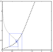
Figure 5: Stability of spiderweb ($v_{s}=0.4$)

It is evident that there is global convergence of the discrete iteration. Hence no oscillations can arise, even under arbitrary delays in the feedback from $P_{N}$ to $M$, and in fact that all solutions converge to a unique equilibrium.

On the other hand, for a larger value of $v_{s}$, such as $v_{s}=0.5$, the discrete iteration conditions are violated; see Figure 6 for the “spiderweb diagram” that shows divergence of the discrete iteration.

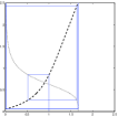
Figure 6: Instability of spiderweb ($v_{s}=0.5$)

Thus, one may expect periodic orbits in this case. We next prove a result that shows that indeed that happens.

6 Periodic Behavior when SGT Conditions Fail

One may conjecture that there is a connection between periodic behaviors of the original system, at least under delayed feedback, and of the associated discrete iteration. We first present an informal discussion and then give a precise result.

For simplicity, let us suppose that $k$ already denotes the composition of the characteristics $g$ and $k$. The input values $u$ with $k(k(u))=u$ which do not arise from the unique fixed point of $k(u)=u$ are period-two orbits of the iteration $u^{+}=k(u)$. Now suppose that we consider the delay differential system $\dot{x}(t)=f(x(t),h(x(t-r)))$, where the delay $r>0$ is very large. We take the initial condition $x(t)=x_{0}$, $t\in[-r,0]$, where $x_{0}$ is picked in such a manner that $h(x_{0})=u_{0}$, and $u_{0}\not=u_{1}$ are two elements of $U$ such that $k(u_{0})=u_{1}$ and $k(u_{1})=u_{0}$. If the input to the open-loop system $\dot{x}=f(x,u)$ is $u(t)\equiv u_{0}$, then the definition of characteristic says that the solution $x(t)$ approaches $x_{1}$, where $h(x_{1})=u_{1}$, Thus, if the delay length $r$ is large enough, the solution of the closed-loop system will be close to the constant value $x_{1}$ for $t\approx r$. Repeating this procedure, one can show the existence of a lightly damped “oscillation” between the values $x_{0}$ and $x_{1}$, in the sense of a trajectory that comes close to these values as many times as desired (a larger $r$ being in principle required in order to come closer and more often). In applications in which measurements have poor resolution and time duration, it may well be impossible to practically determine the difference between such pseudo-oscillations and true oscillations.

It is an open question to prove the existence of true periodic orbits, for large enough delays, when the small-gain condition fails. The problem is closely related to questions of singular perturbations for delay systems, by time-re-parametrization. We illustrate this relation by considering the scalar case, and with $y=x$. The system $\dot{x}=f(x,x(t-r))$, has periodic orbits for large enough $r$ if and only if the system $\varepsilon\dot{x}(t)=f(x(t),x(t-1))$ has periodic orbits for small enough $\varepsilon>0$. For $\varepsilon=0$, we have the algebraic equation $f(x,u)=0$ that defines the characteristic $x=k(u)$. Thus one would want to know that periodic orbits of the iteration $u^{+}=k(u)$, seen as the degenerate case $\varepsilon=0$, survive for small $\varepsilon>0$. A variant of this statement is known in dimension one from work of Nussbaum and Mallet-Paret ([29]), which shows the existence of a continuum of periodic orbits which arise in a Hopf bifurcation and persist for $0<\varepsilon\ll 1$; see also the more recent work [22]. (We thank Hal Smith for this observation.)

We now show that, at least, for a class of systems which is of some general interest in biology, and which contains the circadian model, oscillations can be proved to exist if delays are large enough and the SGT fails locally (exponential instability of the discrete iteration).

6.1 Predicting Periodic Orbits when the Condition Fails

In this section we prove the following theorem, which applies immediately to the complete circadian model (14).

Theorem 2

Consider a tridiagonal system $\dot{x}=f(x,u)$ with scalar input $u$:

$$\begin{array}[]{rcl}\dot{x}_{1}&=&f_{1}(x_{1},x_{2},u)\\ \dot{x}_{2}&=&f_{2}(x_{1},x_{2},x_{3})\\ &\vdots&\\ \dot{x}_{n-1}&=&f_{n-1}(x_{n-2},x_{n-1},x_{n})\\ \dot{x}_{n}&=&f_{n}(x_{n-1},x_{n})\end{array}$$ (18)

and scalar output $y=x_{n}$. The functions $f_{i}$ are twice continuously differentiable, and (cooperativity) all the off-diagonal Jacobian entries are positive. Suppose that there is a unique pair $(x_{0},u_{0})\in{\mathbb{R}}^{n}\times{\mathbb{R}}$ such that $f(x_{0},u_{0})=0$, and consider the linearized system $(A,b,c)$, where $b=(1,0,\ldots,0,0)^{\prime}$, $c=(0,0,\ldots,0,1)$, and $A=D_{x}f$, the Jacobian of the vector field $f(x,u_{0})$ evaluated at $x_{0}$. Assume that $A$ is nonsingular, and let $g=c(-A)^{-1}b$ be the DC gain of the linearized system. Pick any positive number $k$ such that $kg>1$, and consider a delayed feedback $u(t)=-ky(t-h)$ with $h>0$. Then, for some $h>0$, the system (18) under the feedback $u(t)=-ky(t-h_{0})$ admits a periodic solution, and, moreover, the omega-limit set of every bounded solution is either a periodic orbit, the origin, or a nontrivial homoclinic orbit with $\lim_{t\rightarrow\pm\infty}=x_{0}$.

Note that the uniqueness result for closed-loop equilibria will always hold in our case, and the DC gain property $kg>1$ corresponds to a locally unstable discrete iteration. The matrix $A$ is Hurwitz when we have hyperbolicity and parameters as considered earlier (existence of characteristics). The conclusion is that, for a suitable delay length $h_{0}$, there is at least one periodic orbit, and, moreover, bounded solutions not converging to zero exhibit oscillatory behavior (with periods possibly increasing to infinity, if the omega-limit set is a homoclinic orbit). (We conjecture that moreover, for the circadian example, in fact almost all solutions converge to a periodic orbit. Proving this would require establishing that no homoclinic orbits exist for our systems, just as shown, when no delays present, in [28].)

Before proving Theorem 2, we show the following simple lemma about linear systems.

Lemma 6.1

Consider a linear $n$-dimensional single-input single-output system $(A,b,c)$, with $b=(1,0,\ldots,0,0)^{\prime}$ and $c=(0,0,\ldots,0,1)$, and suppose that $A$ is a linear tridiagonal matrix

$$A\;=\;\pmatrix{d_{1}&b_{2}&0&0&\ldots&0&0\cr a_{2}&d_{2}&b_{3}&0&\ldots&0&0\cr 0&a_{3}&d_{3}&b_{4}&\ldots&0&0\cr\cdot&\cdot&\cdot&\cdot&\ldots&\cdot&\cdot\cr\cdot&\cdot&\cdot&\cdot&\ldots&\cdot&\cdot\cr 0&0&0&0&\ldots&a_{n}&d_{n}}$$

with $a_{i}b_{i}>0$ for all $i$ (in particular, this holds if all off-diagonal elements are positive). Then, the transfer function $W(s)=c(sI-A)^{-1}b$ has no zeroes and has distinct real poles; more specifically, $W(s)=\frac{p_{0}}{q(s)}$, where $p_{0}=a_{2}\ldots a_{n}$ and $q(s)=(s-\alpha_{1})\ldots(s-\alpha_{n})$ for distinct real numbers $\alpha_{1},\ldots,\alpha_{n}$. Moreover, there are two real-valued functions $\mu:{\mathbb{C}}\rightarrow{\mathbb{R}}$ and $\nu:{\mathbb{C}}\rightarrow{\mathbb{R}}_{>0}$ so that the logarithmic derivative $Q(s)=q^{\prime}(s)/q(s)$ satisfies $Q(s)=\mu(s)-i\nu(s){\mbox{Im}s}$ for every $s$ that is not a root of $q$.

Proof. The fact that $A$ has $n$ distinct real eigenvalues is a classical one in linear algebra; we include a short proof to make the paper more self-contained. Pick any positive number $\sigma_{1}$ and define, inductively,

$$\sigma_{i}\,:=\;\sigma_{i-1}\sqrt{\frac{a_{i}}{b_{i}}}$$

for $i=2,\ldots,n$. Let $S=\mbox{diag}\,\left(\sigma_{1},\ldots,\sigma_{n}\right)$. Then $B=S^{-1}AS$ is a tridiagonal symmetric matrix:

$$B\;=\;\pmatrix{d_{1}&c_{2}&0&0&\ldots&0&0\cr c_{2}&d_{2}&c_{3}&0&\ldots&0&0\cr 0&c_{3}&d_{3}&c_{4}&\ldots&0&0\cr\cdot&\cdot&\cdot&\cdot&\ldots&\cdot&\cdot\cr\cdot&\cdot&\cdot&\cdot&\ldots&\cdot&\cdot\cr 0&0&0&0&\ldots&c_{n}&d_{n}}$$

where $c_{i}=\varepsilon_{i}\sqrt{a_{i}b_{i}}$ and $\varepsilon_{i}=\mbox{sign}\,a_{i}=\mbox{sign}\,b_{i}\in\{-1,+1\}$. Therefore $B$, and hence also $A$, has all its eigenvalues real. Moreover, there is a basis $\{v_{1},\ldots,v_{n}\}$ consisting of orthogonal eigenvectors of $B$, and so $A$ admits the linearly independent eigenvectors $Sv_{i}$. Moreover, all eigenvalues of $B$ (and so of $A$) are distinct. (Pick any $\lambda$ and consider $C:=B-\lambda I$. The first $n-1$ rows of $C$ look just like those of $B$, with $d_{i}:=d_{i}-\lambda$. The $n-1\times n$ matrix consisting of these rows has rank $n-1$ (just consider its last $n-1$ columns, a nonsingular matrix), so it follows that $C$ has rank$\geq n-1$. Therefore, the kernel of $C$ has dimension at most one.) We conclude that $A$ has $n$ distinct real eigenvalues and hence its characteristic polynomial has the form $q(s)=(s-\alpha_{1})\ldots(s-\alpha_{n})$.

By Cramer’s rule, $(sI-A)^{-1}=(1/q(s))\mbox{cof}(sI-A)$, where “cof” indicates matrix of cofactors. Thus $W(s)=p_{0}/q(s)$, where $p_{0}$ is the $(n,1)$ entry of $\mbox{cof}(sI-A)$, i.e. $(-1)^{n+1}$ times the determinant of the matrix $\widetilde{(sI-A)}_{1,n}$ obtained by deleting from $sI-A$ the first row and last column. The matrix $\widetilde{(sI-A)}_{1,n}$ is upper triangular, and its determinant is $(-a_{2})\ldots(-a_{n})=(-1)^{n-1}a_{2}\ldots a_{n}$. Therefore $p_{0}=a_{2}\ldots a_{n}$, as claimed.

Finally, consider $Q(s)=\sum_{k=1}^{n}\frac{1}{s+\alpha_{k}}$. Write $s=a+ib$, so that

$$\frac{1}{s+\alpha_{k}}=\frac{1}{(a+\alpha_{k})+ib}=\frac{(a+\alpha_{k})-ib}{\rho_{k}}$$

where $\rho_{k}=(a+\alpha_{k})^{2}+b^{2}$, and therefore

$$Q(s)\;=\;\sum_{k=1}^{n}\frac{a+\alpha_{k}}{\rho_{k}}\,-\,i\left(\sum_{k=1}^{n}\frac{1}{\rho_{k}}\right)b\;=\;\mu(s)-i\nu(s)b$$

as desired.  

We now continue the proof of Theorem 2, by first studying the closed-loop linearized system $\dot{x}(t)=Ax(t)+bkcx(t-h)$. The closed-loop transfer function

$$W_{h}=\frac{W}{1+ke^{-hs}W(s)}$$

corresponding to a negative feedback loop with delay $h$ and gain $k$, simplifies to:

$$W_{h}=\frac{p_{0}}{F}\,,\quad\quad F(s,h)=q(s)+pe^{-hs},$$

where $p=p_{0}k$.

In order to prove that there are oscillatory solutions for some $h=h_{0}$, we proceed as follows. We will use the weak form of the Hopf bifurcation theorem (“weak” in that no assertions are made regarding super or subcriticality of the bifurcation) as given in Theorem 11.1.1 in [18]. The theorem guarantees that oscillatory solutions will exist, for the nonlinear system, and for some value of the delay $h$ arbitrarily close to a given $h_{0}>0$, provided that the following two properties hold for $h_{0}$:

(H1) There is some $\omega_{0}\not=0$ such that $F(i\omega_{0},h_{0})=0$, $\omega=i\omega_{0}$ is a simple root of $F(\omega,h_{0})=0$, and (nonresonance) $F(mi\omega,h_{0})\not=0$ for all integers $m>1$;

and letting $\lambda(h)$ be a ${\cal C}^{1}$ function such that $F(\lambda(h),h)=0$ for all $h$ near $h_{0}$ and $\lambda(h_{0})=\omega_{0}$ (such a function always exists):

(H2) $\mbox{Re}\,\lambda^{\prime}(h_{0})\not=0$.

In order to prove these properties, we proceed analogously to what is done for cyclic systems in [9]. (Cyclic systems are the special case in which $\partial f_{i}/\partial x_{i+1}\equiv 0$ for each $i=1,\ldots,n-1$, which is not the case in our circadian system.)

We first show that $F(i\omega_{0},h_{0})=0$ for some $h_{0}>0$ and $\omega_{0}>0$. Since $q(s)F(s,h)=1+(p/q(s))e^{-hs}$ and $q(i\omega)\not=0$ for all real numbers $\omega$ (because $q$ has only real roots, and $A$ is nonsingular, so also $q(0)\not=0$), it is enough to find an $h_{0}>0$ and $\omega_{0}>0$ such that $f(\omega_{0})=-e^{ih_{0}\omega_{0}}=e^{i(h_{0}\omega_{0}-\pi)}$, where $f(\omega)=p/q(i\omega)$. Since $f$ is a continuous function on $[0,\infty)$, $f(0)=p_{0}k/q(0)=W(0)k=gk>1$ by assumption, and $\lim_{\omega\rightarrow\infty}f(\omega)=0$, there is some $\omega_{0}>0$ such that $|f(\omega)|=1$, so that $f(\omega)=e^{i\varphi}$ for some $\varphi$ which we may take in the interval $(0,2\pi]$. It thus suffices to pick $h_{0}=\varphi+\pi/\omega_{0}$, so that $h_{0}\omega_{0}-\pi=\varphi$.

Fix any such $h_{0}$. Since for retarded delay equations there are at most a finite number of roots on any vertical line, we can pick $\omega_{0}$ with largest possible magnitude, so that $F(mi\omega_{0},h_{0})\not=0$ for all integers $m>1$. To prove that (H1) and (H2) hold for these $h_{0}$ and $\omega_{0}$, we first prove that $(dF/ds)(i\omega,h)$ is nonzero at each point $i\omega$ in the imaginary axis, and all $h>0$ (so, in particular, at $(i\omega_{0},h_{0})$). By the implicit function theorem, this will imply that $\omega_{0}$ is a simple root, as needed for (H1). Since $F(\lambda(h),h))\equiv 0$ in a neighborhood of $h_{0}$, we also have that

$$\lambda^{\prime}(h) = -\frac{\partial F}{\partial h}(\lambda(s),h)\,/\,\frac{\partial F}{\partial s}(\lambda(s),h)$$

$$= \frac{spe^{-hs}}{q^{\prime}(s)-hpe^{-hs}}\;=\;\frac{s}{\frac{q^{\prime}(s)}{pe^{-hs}}-h}\,.$$

At $\omega=\omega_{0}$ and $h=h_{0}$, we have that $F(\omega,h)=0$, so $q(s)=-pe^{-hs}$, and therefore, denoting $Q(s):=q^{\prime}(s)/q(s)$:

$$\lambda^{\prime}(h_{0})\;=\;-\frac{i\omega_{0}}{Q(i\omega_{0})+h_{0}}\,.$$

It follows that, for $\omega_{0}>0$:

$$\mbox{Re}\,\lambda^{\prime}(h_{0}) = \mbox{Im}\,\frac{1}{Q(i\omega)+h_{0}}$$

$$= -\mbox{Im}\,\left[Q(i\omega_{0})+h_{0}\right]\;=\;-\mbox{Im}\,Q(i\omega_{0})\,.$$

The proof that periodic orbits exist, for each $h$ near enough $h_{0}$, will then be completed if we show that $\mbox{Im}\,Q(i\omega)\not=0$ for all nonzero real numbers $\omega$. But, indeed, Lemma 6.1 says that $Q(i\omega)=\mu(i\omega)-i\nu(i\omega)\omega$, where $\nu(i\omega)>0$, so $\mbox{Im}\,Q(i\omega)=-\nu(i\omega)\omega\not=0$.

To conclude the proof, we note that the conclusion about global behavior follows from the Poincaré-Bendixson for delay-differential tridiagonal systems due to Mallet-Paret and Sell [27].  

Note that, since $\mbox{Re}\,\lambda^{\prime}(h_{0})\not=0$, if $h_{0}^{\prime}$ is near enough $h_{0}$, then the system (18) under negative feedback $u=-ky(t-h_{0}^{\prime})$ admits a pair of complex conjugate eigenvalues $a+i\omega$ for its linearization, with $a>0$. Thus, its equilibrium is exponentially unstable, and therefore every bounded solution not starting from the center-stable manifold will in fact converge to either a homoclinic orbit involving the origin or a periodic orbit.

6.2 Examples

As a first example, we take the system with the parameters that we have considered, and $v_{s}=0.5$. We have seen that the spider-web diagram suggests oscillatory behavior when delays are present in the feedback loop. We first compute the equilibrium of the closed-loop system (with no delay), which is approximately:

$$M\approx 1.47,P_{1}=0.42,P_{2}=0.29,P_{0}=0.71,P_{N}=0.42.$$

We now consider the system with variables $M,P_{1},P_{2},P_{3},P_{N}$ in which the feedback term $v_{s}K_{I}^{n}/(K_{I}^{n}+P_{3}^{n})$ is replaced by an input $u$. Let $A$ be the Jacobian of this open-loop dynamics evaluated at the positive equilibrium given above. Then $sI-A\approx$

$$\left[\begin{array}[]{ccccc}0.08+s&0&0&0&0\\ \vskip 6.0pt plus 2.0pt minus 2.0pt\cr-0.38&0.87+s&-0.54&0&0\\ \vskip 6.0pt plus 2.0pt minus 2.0pt\cr 0&-0.87&2.24+s&-0.96&0\\ \vskip 6.0pt plus 2.0pt minus 2.0pt\cr 0&0&-1.70&3.66+s&-1.3\\ \vskip 6.0pt plus 2.0pt minus 2.0pt\cr 0&0&0&-1.9&1.3+s\end{array}\right]$$

and hence the transfer function $W(s)=c(sI-A)^{-1}b$, where $b=(1,0,0,0,0)^{\prime}$ and $c=(0,0,0,0,1)$, is:

$$W(s)=\frac{p_{0}}{q(s)},$$

where $p_{0}\approx 1.075$ and $q(s)\approx$

$$\left(0.084+s\right)\left({s}^{4}+8.08\,{s}^{3}+17.61\,{s}^{2}+10.98\,s+1.56\right).$$

The DC gain of the system is $g=W(0)\approx 8.26$ (which is positive, as it should be since the open loop system is monotone and has a well-defined steady-state characteristic). and $k=-\partial(v_{s}K_{I}^{n}/(K_{I}^{n}+P_{3}^{n})/\partial P_{3}\approx 0.14$ when evaluated at the computed equilibrium. Thus $f(0)=gk\approx 1.138>1$, as required. Indeed, $\mbox{Im}\,Q(i\omega)\approx$

$$\frac{-\left(2.88+133.26\,\omega^{2}+408.07\,\omega^{4}+120.12\,\omega^{6}+5.0\,\omega^{8}\right)\omega}{\left(0.007+\omega^{2}\right)\left(2.42+65.68\omega^{2}+135.81\omega^{4}+30.02\omega^{6}+\omega^{8}\right)}$$

and hence $\mbox{Im}\,Q(i\omega)\not=0$ for all $\omega\not=0$.

We show in Figure 7 one simulation, with $h=100$, showing a periodic limit cycle.

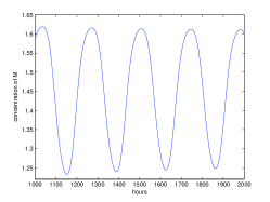
Figure 7: Oscillations seen in simulations ($v_{s}=0.5$, delay $=100$hr, initial conditions all at $0.2$), using MATLAB’s dde23 package

The delay length needed for oscillations when $v_{s}=0.5$ is biologically unrealistic, so we also show simulations for $v_{2}=0.6$, a value for which no oscillations occur without delays, but for which oscillations (with a period of about 27 hours) occur when the delay length is about 1 hour, see Figure 8.

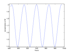
Figure 8: Oscillations seen in simulations ($v_{s}=0.6$, delay $=1$hr, initial conditions all at $0.2$), using MATLAB’s dde23 package

7 A Counterexample

We now provide a (non-monotone) system as well as a feedback law $u=g(y)$ so that:

• the system has a well-defined and increasing characteristic $k$,

• the discrete iteration $u^{+}=g(k(u))$ converges globally, and solutions of the closed-loop system are bounded,

yet a stable limit-cycle oscillation exists in the closed-loop system. This establishes, by means of a simple counterexample, that monotonicity of the open-loop system is an essential assumption in our theorem. Thus, robustness is only guaranteed with respect to uncertainty that preserves monotonicity of the system.

The idea underlying the construction is very simple. The open-loop system is linear, and has the following transfer function:

$$W(s)=\frac{-s+1}{s^{2}+(0.25)s+1}\,.$$

Since the DC gain of this system is $W(0)=1$, and the system is stable, there is a well-defined and increasing characteristic $k(u)=u$. However a negative feedback gain of $1/2$ destabilizes the system, even though the discrete iteration $u^{+}=(-1/2)u$ is globally convergent. (The $H_{\infty}$ gain of the system is, of course, larger than $1$, and therefore the standard small-gain theorem does not apply.) In state-space terms, we use this system:

$$\dot{x}_{1} = (-1/4)x_{1}-x_{2}+2u$$

$$\dot{x}_{2} = x_{1}$$

$$y = (1/2)(x_{2}-x_{1})\,.$$

Note that, for each constant input $u\equiv u_{0}$, the solution of the system converges to $(0,u_{0}/2)$, and therefore the output converges to $u_{0}$, so indeed the characteristic $k$ is the identity.

We only need to modify the feedback law in order to make solutions of the closed-loop globally bounded. For the feedback law we pick $g(x)=-0.5\mbox{sat}(y)$, where $\mbox{sat}(\cdot):=\mbox{sign}(\cdot)\min\{1,|\cdot|\}$ is a saturation function. The only equilibrium of the closed-loop system is at $(0,0)$.

The discrete iteration is

$$u^{+}=-(1/2)\mbox{sat}(u)\,.$$

With an arbitrary initial condition $u_{0}$, we have that $u_{1}=-(1/2)\mbox{sat}(u_{0})$, so that $|u_{1}|\leq 1/2$. Thus $u_{k}=(-1/2)u_{k-1}$ for all $k\geq 2$, and indeed $u_{k}\rightarrow 0$ so global convergence of the iteration holds.

However, global convergence to equilibrium fails for the closed-loop system, and in fact there is a periodic solution. Indeed, note that trajectories of the closed loop system are bounded, because they can be viewed as solutions of a stable linear system forced by a bounded input. Moreover, since the equilibrium is a repelling point, it follows by the Poincaré-Bendixson Theorem that a periodic orbit exists. Figure 9 is a simulation showing a limit cycle.

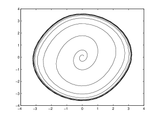
Figure 9: Limit cycle in counterexample

References

- [1] D. Angeli and E.D. Sontag, “Monotone control systems,” IEEE Trans. Autom. Control 48(2003): 1684–1698.
- [2] D. Angeli and E.D. Sontag, “Multi-stability in monotone Input/Output systems,” Systems and Control Letters, 51(2004): pp. 185–202. (Summarized version: ”A note on multistability and monotone I/O systems,” in Proc. IEEE Conf. Decision Control, Maui, 2003.)
- [3] D. Angeli and E.D. Sontag, “Interconnections of monotone systems with steady-state characteristics,” In Optimal control, stabilization and nonsmooth analysis, volume 301 of Lecture Notes in Control and Inform. Sci., pages 135–154. Springer, Berlin, 2004.
- [4] D. Angeli, P. de Leenheer, and E.D. Sontag, “A small-gain theorem for almost global convergence of monotone systems,” Systems Control Lett., 52(5):407–414, 2004.
- [5] Chisci, L. and Falugi, P., “Asymptotic tracking for constrained monotone systems,” IEEE Trans. Autom. Control, 51 (2006): 873-879.
- [6] E.N. Dancer, “Some remarks on a boundedness assumption for monotone dynamical systems,” Proc. of the AMS, 126:801–807, 1998.
- [7] P. de Leenheer, D. Angeli, and E.D. Sontag, “On predator-prey systems and small-gain theorems,” Math. Biosci. Eng., 2(1):25–42, 2005.
- [8] G. Enciso and E.D. Sontag, “Monotone systems under positive feedback: multistability and a reduction theorem,” Systems Control Lett., 54(2):159–168, 2005.
- [9] G. Enciso, “A dichotomy for a class of cyclic delay systems,” Mathematical Biosciences, to appear, 2007. (Also Arxiv, q-bio.MN/0601015),
- [10] G. Enciso, H.L. Smith, and E.D. Sontag, “Non-monotone systems decomposable into monotone systems with negative feedback,” J. Differential Equations 2005, in press.
- [11] G. Enciso and E.D. Sontag, “Global attractivity, I/O monotone small-gain theorems, and biological delay systems,” Discrete and Continuous Dynamical Systems, in press.
- [12] G. Enciso and E.D. Sontag, “On the stability of a model of testosterone dynamics,” J. Mathematical Biology 49(2004), pp. 627–634.
- [13] T. Gedeon and E.D. Sontag, “Oscillations in multi-stable monotone systems with slowly varying feedback,” J. of Differential Equations, page to appear, 2007.
- [14] A. Goldbeter, “A model for circadian oscillations in the Drosophila period protein (PER),” Proc. Royal Soc. Lond. B. 261(1995): 319–324.
- [15] A. Goldbeter, Biochemical Oscillations and Cellular Rhythms, Cambridge Univ. Press, Cambridge, 1996.
- [16] F. Grognard, Y. Chitour, G. Bastin, “Equilibria and stability analysis of a branched metabolic network with feedback inhibition,” AIMS Journal on Network and Heterogeneous Media (NHM) 1(2006): 219-239.
- [17] D. Gromov and J. Raisch, “Detecting and enforcing monotonicity for hybrid control systems synthesis,” in Proc. 2nd IFAC Conf. on Analysis and Design of Hybrid Systems (Alghero, Italy), 7-9 June 2006.
- [18] J.K. Hale and S.M. Verduyn Lunel, Introduction to Functional Differential Equations, Springer, NY, 1993.
- [19] M. Hirsch, “Differential equations and convergence almost everywhere in strongly monotone flows,” Contemporary Mathematics, 17:267–285, 1983.
- [20] M. Hirsch, “Systems of differential equations that are competitive or cooperative ii: Convergence almost everywhere,” SIAM J. Mathematical Analysis, 16:423–439, 1985.
- [21] M. Hirsch and H.L. Smith, “Monotone dynamical systems,” In Handbook of Differential Equations, Ordinary Differential Equations (second volume). Elsevier, Amsterdam, 2005.
- [22] A.F. Ivanov, and B. Lani-Wayda, “Periodic solutions for three-dimensional non-monotone cyclic systems with time delays”, Discrete and Continuous Dynamical Systems, A 11 (2004): 667–692.
- [23] J.F. Jiang, “On the global stability of cooperative systems,” Bulletin of the London Math Soc, 6:455–458, 1994.
- [24] J.-C. Leloup, and A. Goldbeter, “A model for circadian rhythms in Drosophila incorporating the formation of a complex between the PER and TIM proteins”, J. Biol. Rhythms , Vol. 13, pp. 70-87, 1998.
- [25] J.-C. Leloup, and A. Goldbeter, “Chaos and birhythmicity in a model for circadian oscillations of the PER and TIM proteins in Drosophila”, J. Theor. Biol. , Vol. 198, pp. 445-459, 1999.
- [26] M. Malisoff and P. De Leenheer, “A small-gain theorem for monotone systems with multivalued input-state characteristics,” IEEE Trans. Automat. Control 51(2006): 287–292.
- [27] Mallet-Paret, J. and Sell, G. R., “The Poincaré-Bendixson Theorem for Monotone Cyclic Feedback Systems with Delay”, Journal of differential equations, Vol. 125, pp. 441-489, 1996.
- [28] J. Mallet-Paret and H. Smith, “The Poincare-Bendixon theorem for monotone cyclic feedback systems,” J. Dynamics and Diff. Eqns , 2(1990): 367-421.
- [29] J. Mallet-Paret and R. Nussbaum, “Global continuation and asymptotic behaviour for periodic solutions of a differential-delay equation,” Ann. Mat. Pura Appl., 145 (1986): 33–128.
- [30] H. Schneider and M. Vidyasagar, “Cross-positive matrices,” SIAM J. Numer. Anal., 7:508–519, 1970.
- [31] J. Smillie, “Competitive and cooperative tridiagonal systems of differential equations,” SIAM J. Math. Anal. 15(1984): pp. 530–534.
- [32] H.L. Smith, Monotone Dynamical Systems: an Introduction to the Theory of Competitive and Cooperative systems, Mathematical Surveys and Monographs, Vol. 41, American Mathematical Society, Ann Arbor, 1995.
- [33] H.L. Smith, “Periodic tridiagonal competitive and cooperative systems of differential equations,” SIAM J. Math. Anal.22(1991): 1102-1109.
- [34] E.D. Sontag, “Molecular systems biology and control,” Eur. J. Control, 11(4-5):396–435, 2005.
- [35] P. Volkmann, “Gewohnliche differentialungleichungen mit quasimonoton wachsenden funktionen in topologischen vektorraumen,” Math. Z., 127:157–164, 1972.
- [36] S. Walcher, “On cooperative systems with respect to arbitrary orderings,” Journal of Mathematical Analysis and Appl., 263:543–554, 2001.
- [37] W. Walter, “Differential and Integral Inequalities,” Springer-Verlag, Berlin, 1970.