Spatiotemporal complexity of a ratio-dependent predator-prey system

Abstract

In this paper, we investigate the emergence of a ratio-dependent predator-prey system with Michaelis-Menten-type functional response and reaction-diffusion. We derive the conditions for Hopf, Turing and Wave bifurcation on a spatial domain. Furthermore, we present a theoretical analysis of evolutionary processes that involves organisms distribution and their interaction of spatially distributed population with local diffusion. The results of numerical simulations reveal that the typical dynamics of population density variation is the formation of isolated groups, i.e., stripelike or spotted or coexistence of both. Our study shows that the spatially extended model has not only more complex dynamic patterns in the space, but also chaos and spiral waves. It may help us better understand the dynamics of an aquatic community in a real marine environment.

I Introduction

Ecological systems are characterized by the interaction between species and their natural environment Baurmann et al. (2006). Such interaction may occur over a wide range of spatial and temporal scales Neuhauser (2001); Levin et al. (1997). The study of complex population dynamics is nearly as old as population ecology. In the 1920s, Lotka and Volterra independently developed a simple model of interacting species that still bears their joint names. This was a nearly linear model, but the predator-prey version displayed neutrally stable cycles May (1976); Kendall (2001). From then on, the dynamic relationship between predators and their prey has long been and will continue to be one of dominant themes in both ecology and mathematical ecology due to its universal existence and importance Berryman (1992); Kuang and Beretta (1998); Murray (3 edition, 2003).

Predator-prey models follow two general principles: one is that population dynamics can be decomposed into birth and death processes; the other is the conservation of mass principle, stating that predators can grow only as a function of what they have eaten Jost (1998). With these two principles we can write the canonical form of a predator-prey system as

$$\left\{\begin{array}[]{l}\dot{x}(t)=xg(x)-f(x,y)y-\mu_{x}(x)x,\\[8.0pt] \dot{y}(t)=\gamma f(x,y)y-\mu_{y}(y)y.\\ \end{array}\right.$$ (3)

where $g(x)$ is the per capita prey growth rate in the absence of the predator, $\mu_{x}$ and $\mu_{y}$ are natural mortalities of prey and predator respectively, $f(x,y)$ is the functional response. And $\gamma f(x,y)$ is the per capita production of predator due to predation, which is often called the numerical response. The functional response plays a main role in system (3): the knowledge of this function determines the dynamics of the whole system and the transfer of the biomass in the predation because it is proportional to the numerical response. Usually one considers consumption to be the major death cause for the prey. In this case $\mu_{x}(x)$ can be neglected and set to 0 (as long as the predator exists) Jost (1998).

In population dynamics, a functional response of the predator to the prey density refers to the change in the density of prey attached per unit time per predator as the prey density changes Ruan and Xiao (2001). In general, functional response can be classified as: (i) prey dependent, when prey density alone determines the response, i.e., $f(x,y)=p(x)$; (ii) predator dependent, when both predator and prey populations affect the response. Particularly, when $f(x,y)=p(\frac{x}{y})$, we call model (3) strictly ratio-dependent; and (iii) multi-species dependent, when species other than the focal predator and its prey species influence the functional response Abrams and Ginzburg (2000). Differing from the prey-dependent predator-prey models, the ratio-dependent predator-prey systems have two principal predictions: (a) equilibrium abundances are positively correlated along a gradient of enrichment and (b) the “paradox of enrichment” either completely disappears or enrichment is linked to stability in a more complex way Arditi and Ginzburg (1989); Rosenzweig (1971). The ratio-dependent predator-prey model has been studied by several researchers recently and very rich dynamics have been observed Arditi and Ginzburg (1989); Kuang and Beretta (1998); Jost et al. (1999); Murray (3 edition, 2003); Xiao and Jennings (2005).

On the other hand, pattern formation in nonlinear complex systems is one of the central problems of the natural, social, and technological sciences Medvinsky et al. (2002). In particular, starting with the pioneering work of Segel and Jackson Segel and Jackson (1972), spatial patterns and aggregated population distributions are common in nature and in a variety of spatio-temporal models with local ecological interactions Baurmann et al. (2006); Pascual (1993). Promulgated by the theoretical paper of Turing Turing (1952), the field of research on pattern formation modeled by reaction-diffusion systems, which provides a general theoretical framework for describing pattern formation in systems from many diverse disciplines including (but not limited to) biology Klausmeier (1999); Medvinsky et al. (2002); Liu et al. (2006); von Hardenberg et al. (2001); Lejeune et al. (2002); Sharon et al. (2004); Pascual et al. (2002), chemistry Ouyang and Swinney (1991); Vanag et al. (2000); Yang et al. (2002a, b); Yang and Epstein (2003, 2004), physics Just et al. (2001); Cross and Hohenberg (1993); Yochelis et al. (2002); Leppänen et al. (2004), and so on, seems to be a new increasingly interesting area, particularly during the last decade.

In Ref. Neuhauser (2001), Neuhauser surveys some current work on spatial mathematical models in ecology. Much of this work consists of building spatial dimensions into existing classical models, such as the Lotka-Volterra model that describes competition between species. But the research on the spatial pattern of ratio-dependent predator-prey models seems to be rare.

II Stability and Bifurcation analysis

In this paper, we mainly focus on the ratio-dependent predator-prey system with Michaelis-Menten-type(or Michaelis-Menten-Holling) functional response:

$$\left\{\begin{array}[]{l}\frac{\partial N}{\partial t}=r(1-\frac{N}{K})N-\frac{\alpha N/P}{1+\alpha hN/P}P+D_{1}\nabla^{2}N\\[8.0pt] \quad\,\,\,\,=r(1-\frac{N}{K})N-\frac{\alpha N}{P+\alpha hN}P+D_{1}\nabla^{2}N,\\[8.0pt] \frac{\partial P}{\partial t}=\gamma\frac{\alpha N}{P+\alpha hN}P-\mu P+D_{2}\nabla^{2}P.\\[8.0pt] \forall(N,P)\in[0,\infty]^{2}\backslash(0,0).\end{array}\right.$$ (8)

where $N,P$ stand for prey and predator density, respectively. $D_{1},D_{2}$ are their respective diffusion coefficients, $\nabla^{2}=\frac{\partial}{\partial x^{2}}+\frac{\partial}{\partial y^{2}}$. All parameters are positive constants, $r$ stands for maximal growth rate of the prey, $\gamma$ conversion efficiency, $\mu$ predator death rate, $K$ carrying capacity, $\alpha$ capture rate and $h$ handling time.

Note that $\frac{\alpha N/P}{1+\alpha hN/P}$ is strictly correct only for $P>0$. In the case of $P=0$ and $N>0$ we can define $f(N,0):=\frac{1}{h}$ (the limit of $f(x)$ for $x\rightarrow\infty$).

Let

$$\begin{array}[]{l}\hat{N}=\frac{\alpha hN}{\gamma K},\quad\hat{P}=\frac{\alpha hN}{\gamma^{2}K},\quad R=\frac{rh}{\gamma},\\[8.0pt] Q=\frac{h\mu}{\gamma},\quad S=\frac{\alpha h}{\gamma},\quad\hat{t}=\frac{\gamma t}{h}.\end{array}$$ (9)

For simplicity we will not write the hat $(\,\hat{}\,)$ in the rest of this paper. And in these new variables, from (8)-(9), we arrive at the following equations containing dimensionless quantities:

$$\left\{\begin{array}[]{l}\frac{\partial N}{\partial t}=R(1-\frac{N}{S})N-\frac{SN}{P+SN}P+D_{1}\nabla^{2}N,\\[8.0pt] \frac{\partial P}{\partial t}=\frac{SN}{P+SN}P-QP+D_{2}\nabla^{2}P.\\ \end{array}\right.$$ (12)

More details about the choice of dimensionless variables in the system (8) as well as possible implications can be found in  Jost et al. (1999).

The dimensionless model (Eq. 12) has only three parameters: $R$, which controls the growth rate of prey; $Q$, which controls the death rate of the predator; and $S$, which measures capturing rate.

The first step in analyzing the model is to determine the behavior of the non-spatial model obtained by setting space derivatives equal to zero. The non-spatial model has at most three equilibria (stationary states), which correspond to spatially homogeneous equilibria of the full model (Eq. 12), in the positive quadrant: $(0,0)$ (total extinct), $(S,0)$ (extinct of the predator) and a nontrivial stationary state $(n^{*},p^{*})$ (coexistence to prey and predator), where

$$\begin{array}[]{l}n^{*}=\frac{S(R+(Q-1)S)}{R},\\[8.0pt] p^{*}=\frac{S(1-Q)}{Q}n^{*}=\frac{{S}^{2}(R-S+QS)(1-Q)}{RQ}\end{array}$$ (13)

Easy to know that $n^{*}$ is positive for all $S<\frac{R}{1-Q}$, which implies $Q<1$ and therefore ensures the positivity of $p^{*}$ Jost et al. (1999).

To perform a linear stability analysis, we linearize the dynamic system (12) around the spatially homogenous fixed point (13) for small space- and time-dependent fluctuations and expand them in Fourier space

$$\begin{array}[]{l}N(\vec{x},t)\sim n^{*}e^{\lambda t}e^{i\vec{k}\cdot\vec{x}},\\[8.0pt] P(\vec{x},t)\sim p^{*}e^{\lambda t}e^{i\vec{k}\cdot\vec{x}}.\end{array}$$ (14)

and obtain the characteristic equation

$$|A-k^{2}D-\lambda I|=0,$$ (15)

where

$$D=\left(\begin{array}[]{cc}D_{1}&0\\ \vskip 6.0pt plus 2.0pt minus 2.0pt\cr 0&D_{2}\end{array}\right),$$ (16)

and $A$ is given by

$$A=\left(\begin{array}[]{cc}\partial_{N}f&\partial_{P}f\\ \vskip 6.0pt plus 2.0pt minus 2.0pt\cr\partial_{N}g&\partial_{P}g\end{array}\right)_{(n^{*},p^{*})}=\left(\begin{array}[]{cc}f_{N}&f_{P}\\ \vskip 6.0pt plus 2.0pt minus 2.0pt\cr g_{N}&g_{P}\end{array}\right),$$ (17)

where the elements are the partial derivatives of the reaction kinetics evaluated at the stationary state $(n^{*},p^{*})$. Now Eq. (15) can be solved, yielding the so called characteristic polynomial of the original problem (Eq. 12)

$$\lambda^{2}-tr_{k}\lambda+\Delta_{k}=0,$$ (18)

where

$$tr_{k}=f_{N}+g_{P}-k^{2}(D_{1}+D_{2})=tr_{0}-k^{2}(D_{1}+D_{2}),$$ (19)

$$\begin{array}[]{l}\Delta_{k}=f_{N}g_{P}-f_{P}g_{N}-k^{2}(f_{N}D_{2}+g_{P}D_{1})+k^{4}D_{1}D_{2}\\[8.0pt] \quad\,\,\,\,=\Delta_{0}-k^{2}(f_{N}D_{2}+g_{P}D_{1})+k^{4}D_{1}D_{2},\end{array}$$ (20)

The roots of Eq.10 yield the dispersion relation

$$\lambda_{1,2}(k)=\frac{1}{2}\Bigl{(}tr_{k}\pm\sqrt{tr_{k}^{2}-4\Delta_{k}}\,\,\Bigr{)}.$$ (21)

It’s well known that reaction-diffusion systems have led to the characterization of three basic types of symmetry-breaking bifurcations responsible for the emergence of spatiotemporal patterns. The space-independent Hopf bifurcation breaks the temporal symmetry of a system and gives rise to oscillations that are uniform in space and periodic in time. The (stationary) Turing bifurcation breaks spatial symmetry, leading to the formation of patterns that are stationary in time and oscillatory in space. The wave (oscillatory Turing or finite-wavelength Hopf) bifurcation breaks both spatial and temporal symmetry, generating patterns that are oscillatory in space and time Yang et al. (2002a).

The Hopf bifurcation occurs when

$$Im(\lambda(k))\neq 0,\quad Re(\lambda(k))=0\,\,\,at\,\,\,k=0.$$ (22)

then we can get the critical value of Hopf bifurcation parameter $S$ equals

$$S_{H}=\frac{R+Q-Q^{2}}{1-Q^{2}}.$$ (23)

At the Hopf bifurcation threshold, the temporal symmetry of the system is broken and gives rise to uniform oscillations in space and periodic oscillations in time with the frequency

$$\omega_{H}=Im(\lambda(k))=\sqrt{\Delta_{0}}=\sqrt{Q(Q-1)(R-S+QS)},$$

the corresponding wavelength is

$$\lambda_{H}=\frac{2\pi}{\omega_{H}}=\frac{2\pi}{\sqrt{Q(Q-1)(R-S+QS)}}.$$ (24)

The Turing bifurcation occurs when

$$Im(\lambda(k))=0,\quad Re(\lambda(k))=0\,\,\,at\,\,\,k=k_{T}\neq 0.$$ (25)

the critical value of bifurcation parameter $S$ equals

$$S_{T}=\frac{D_{1}D_{2}k_{T}^{4}+(D_{2}R+D_{1}Q(1-Q))k_{T}^{2}+RQ(1-Q)}{Q^{3}-(k_{T}^{2}D_{2}+2)Q^{2}+Q+k_{T}^{2}D_{2}},$$ (26)

where

$$k_{T}^{2}=\sqrt{\frac{\Delta_{0}}{D_{1}D_{2}}},$$

and at the Turing threshold, the spatial symmetry of the system is broken and the patterns are stationary in time and oscillatory in space with the wavelength

$$\lambda_{T}=\frac{2\pi}{k_{T}}.$$ (27)

And the Wave bifurcation occurs when

$$Im(\lambda(k))\neq 0,\quad Re(\lambda(k))=0\,\,\,at\,\,\,k=k_{w}\neq 0.$$ (28)

the critical value of Wave bifurcation parameter $S$ equals

$$S_{W}=\frac{k_{w}^{2}(D_{1}+D_{2})+R+Q-Q^{2}}{1-Q^{2}},$$ (29)

where

$$\begin{array}[]{l}k_{w}^{2}=\frac{Q}{2D_{2}^{2}(Q+1)}\Bigl{(}(D_{1}-D_{2})^{2}Q^{4}-2(D_{1}^{2}+D_{2}^{2})Q^{3}\Bigr{.}\\[8.0pt] +(D_{1}^{2}+D_{2}^{2}\Bigl{.}+6D_{1}D_{2}-4D_{2}^{2}R)Q^{2}-4D_{1}D_{2}Q+4D_{2}^{2}R\Bigr{)}^{1/2}.\end{array}$$

Easy to know that, at the Wave threshold, both spatial and temporal symmetries are broken and the patterns are oscillatory in space and time with the wavelength

$$\lambda_{W}=\frac{2\pi}{k_{w}}.$$ (30)

Linear stability analysis yields the bifurcation diagram with $R=0.5,\,Q=0.6,\,D_{2}=0.2$ shown in Fig. 1.

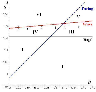
Figure 1: (Color online) Bifurcation diagram for the system (2) with $R=0.5,\,Q=0.6,\,D_{2}=0.2$. Hopf bifurcation line: $S_{H}=\frac{37}{32}$; Turing bifurcation line: $S_{T}=\frac{55}{56}+\frac{55}{28}D_{1}$ with $k_{T}^{2}=5.48571$; Wave bifurcation line: $S_{W}=(\frac{25}{16}D_{1}+\frac{5}{16})k_{W}^{2}+\frac{37}{32}$ with $k_{W}=0.334$. Turing-Hopf bifurcation point: (0.08864, 1.15625) and Turing-Wave bifurcation point: (0.11655, 1.21110).

The Hopf bifurcation line, the Wave bifurcation line and the Turing bifurcation line intersect at two codimension-2 bifurcation points, the Turing-Hopf bifurcation point and the Turing-Wave bifurcation point. The bifurcation lines separate the parametric space into six distinct domains. In domain I, located below all three bifurcation lines, the steady state is the only stable solution of the system. Domain II is region of pure Turing instabilities, and domain III is pure Hopf instabilities. In domain IV, both Hopf and Turing instabilities occur, and in domain V, the Wave and Hopf modes arise. When the parameters correspond to domain VI, which is located above all three bifurcation lines, all three instabilities occur. Fig. 2 shows the dispersion relations of unstable Hopf mode, transition of Turing and Wave modes from stable to unstable. It’s easy to know that all three bifurcations are supercritical.

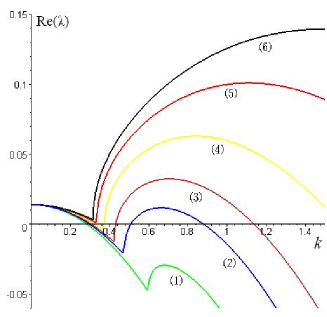
Figure 2: (Color online) Dispersion relations showing unstable Hopf mode, transition of Turing and Wave modes from stable to unstable, e.g., as $D_{1}$ decreased. Parameters: $S=1.2,\,R=0.5,\,Q=0.6,\,D_{2}=0.2$ and (1) $D_{1}$=0.15; (2) $D_{1}$=0.12; (3) $D_{1}$=0.10; (4) $D_{1}$=0.07; (5) $D_{1}$=0.04; (6) $D_{1}$=0.02.

III Spatiotemporal pattern analysis

We have performed extensive numerical simulations of the spatially extended model (12) in two-dimensional space, and the qualitative results are shown here. All our numerical simulations employ the periodic Neumann (zero-flux) boundary conditions with a system size of $200\times 200$ space units and $R=0.5$, $Q=0.6$, $D_{1}=0.02$, $D_{2}=0.2$. The spatiotemporal dynamics of a diffusion-reaction system depends on the choice of initial conditions, which some authors have considered in connection with the problem of biological invasion in a few papers Sherratt et al. (1995); Shigesada and Kawasaki (1997); Petrovskii and Malchow (2001); Medvinsky et al. (2002), where the initial conditions are naturally described by finite functions and the dynamics of the community mainly consists of a variety of diffusive populational fronts. In general, there are two initial conditions used for analysis of the spatial extended systems. One is random spatial distribution of the species, which seems to be more general from the biological point of view (cf. Fig. 3(A) and  4(A),  7(A)); The other is a special choice, i.e., taking the species community in a horizontal layer as decreasing gradually and the vertical distribution of species homogeneous(cf. Fig. 9(A)). In this section we choose the former, and the latter in the next section (IV. Discussion). The equations (12) are solved numerically in two-dimensional space using a finite difference approximation for the spatial derivatives and an explicit Euler method for the time integration with a time stepsize of $\Delta t=0.01$ and space stepsize $\Delta h=0.25$.

From the analysis of section II and phase-transition bifurcation diagram (cf. Fig. 1), the results of computer simulations show that the type of the system dynamics is determined by the values of $S$ and $D_{1}$. We run the simulations until they reach a stationary state or until they show a behavior that does not seem to change its characteristics anymore. For different sets of parameters, the features of the spatial patterns become essentially different if $S$ exceeds a critical value $S_{T}$, $S_{T}$ and $S_{W}$ respectively, they depend on $D_{1}$.

Fig. 3 shows the evolution of the spatial pattern of prey at 0, 5000 and 45000 iterations, with random small perturbation of the stationary solution $n^{*}$ and $p^{*}$ of the spatially homogeneous systems when $S$ is less than the Turing bifurcation threshold $S_{T}$. In this case, one can see that for the system (12), the random initial distribution lead to the formation of a strongly irregular transient pattern in the domain. After the irregular pattern form (cf. Fig. 3(B)) it grows slightly and “jumps” alternately for a certain time, and finally the chaos spiral patterns prevail over the whole domain, and the dynamics of the system does not undergo any further changes (cf. Fig. 3(C) and the addition movie for Fig. 3).

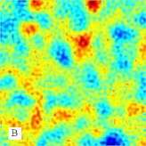
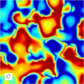
Figure 3: (Color online) Snapshots of contour pictures of the time evolution of the prey at different instants with $S=0.6<S_{T}$. (A) 0 iteration; (B) 5000 iterations; (C) 45000 iterations. [Additional movie format available from the author]

Figures  4 and 5 show spontaneous formation of short stripelike and spotted spatial patterns emerge and coexist stably when the bifurcation parameter $S<S_{T}$ (Fig. 4) and $S_{T}<S<S_{H}$ (Fig. 5). From the snapshots or movies, one can see that the stripelike spatial patterns arise from the random initial conditions. After the stripelike patterns form (cf. Fig. 4(B)) they grow steadily with time until they reach certain width—armlength, and the spatial patterns become distinct. Finally, the stripelike spatial patterns prevail the whole domain (cf. Fig. 4(C) and Fig.5). Comparing the Fig. 4(C) with Fig. 5, we find that the parameter $S$ is closer to $S_{T}$, and the stripelike spatial patterns are more distinct. Here we omit the pre-image of Fig. 5 as they are similar to the Fig. 4(A) and (B). It is easy to see that the stationary patterns are essentially different from the previous case(cf. Fig.3).

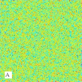
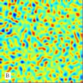
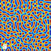
Figure 4: (Color online) Snapshots of contour pictures of the time evolution of the prey at different instants with $S=0.9<S_{T}$. (A) 0 iteration; (B) 5000 iterations; (C) 45000 iterations. [Additional movie format available from the author]

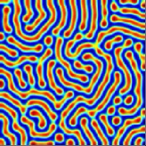
Figure 5: (Color online) Snapshots of contour pictures of the time evolution of the prey at different instants with $S_{T}<S=1.1<S_{H}$ (45000 iterations). [Additional movie format available from the author]

When $S_{H}<S=1.16<S_{W}$, we find that the spotted patterns and the stripelike patterns coexist in the spatially extended model (cf. Fig. 6).

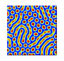
Figure 6: (Color online) Coexistence of stationary spotted patterns and stripelike patterns of the prey for long time run with $S_{H}<S=1.16<S_{W}$. [Additional movie format available from the author]

Fig. 7 shows snapshots of prey spatial pattern at 0, 5000 and 45000 iterations for the parameter $S=1.2>S_{W}$. Although the dynamics of the system starts from the same initial condition as previous cases, there is an essential difference for the spatially extended model (Eq. 12). Form Fig. 7, one can see that the regular spotted patterns prevails over the whole domain at last, and the dynamics of the system does not undergo any further changes (cf. the additional movie for Fig. 7).

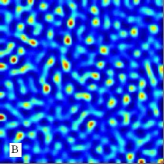
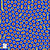
Figure 7: (Color online) Snapshots of contour pictures of the time evolution of the prey at different instants with $S=1.2>S_{W}$. (A) 0 iteration; (B) 5000 iterations; (C) 45000 iterations. [Additional movie format available from the author]

On the other hand, discrete Fourier transform is a basic mathematical tool used to decompose a signal or image into different periodic components. It has been widely used for the spatial patterns Prum and Torres (2003a); Prum et al. (1999); Prum and Torres (2003b). We have also performed numerical investigations into two-dimensional space by Fourier spectra. The numerical computation of the Fourier transform is done by the well-established two-dimensional Fast Fourier Transform (FFT2) algorithm Briggs and Henson (1995). Spatial Fourier transform of the stripelike and spotted patterns in Figures 4(c), 5 and 7(c) are shown as Fig. 8. And digital or digitized transmission electron micrographs (TEMs) are analyzed by using Matlab (Ver.7.0).

From Fig. 8, we find that Fig. 4(C) and Fig. 5 have the same spatial frequency in the length of the space unit and presence of one mode with different wave numbers. On the contrary, Fig. 7(C) has two modes with different wave numbers. The spatial frequency and direction of any component in the power spectrum are given in the length and direction, respectively, of a vector from the origin to the point on the circle. The magnitude is depicted by a gray scale or color scale, but the units are dimensionless values related to the total darkness of the original images. In Fig. 8(mid-hand column), short wavelength, represented by a large circle, corresponds to Turing structures; longer wavelength, represented by a small white circle, corresponds to traveling and/or standing waves. This technique can be particularly appropriate for characterizing quasi-ordered arrays for Fig. 7(C).

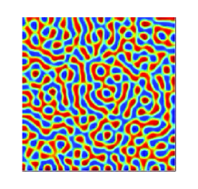
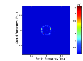
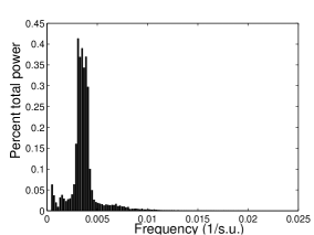
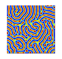
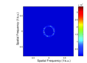
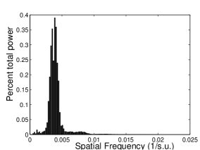
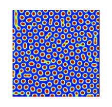
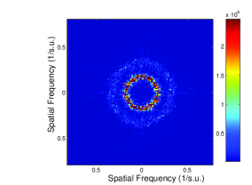
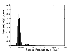
Figure 8: (Color online) Patterns (left-hand column), it spatial Fourier transformation (mid-hand column), and radial average of the power spectrum (right-hand column). Up-row $S=0.9$; Mid-row $S=1.1$; Low-row $S=1.2$.

IV Discussion and conclusion

The numerical results correspond perfectly to our theoretical findings that there are a range of parameters in $S-D_{1}$ plane where the different spatial patterns emerge (cf. Fig. 1). Fig. 1 and the results of simulations present that the chaos patterns will persist in the spatially extended model (Eq. 12) when the parameters are in the domain I. The boundary of this domain can be computed numerically and is shown as the blue line “Turing” in Fig. 1. The stationary state of stripelike patterns exists when the parameters are in the domain II, where its boundary can also be computed numerically and is shown as the black line “Hopf” in Fig. 1. The periodic spotted patterns appear in the domain VI, where the boundary can be computed numerically by the wave bifurcation and is shown as the red line “Wave” in Fig. 1. Moreover, there is transverse domain IV (cf. Fig. 1) in the system between the stripelike patterns and spotted patterns, where the spotted patterns and the stripelike patterns coexist(cf. Fig. 6).

Do the stationary patterns arise dependent on the initial conditions? We test the different initial conditions for the spatially extended system, but the final spatial patterns are the same in qualitative. In those figures we find that the spatial chaos patterns come from the destruction of the spirals, when we choose the special initial condition (cf. Fig. 9) in the domain I. This phenomenon coheres with the results of the study in Refs. Medvinsky et al. (2002); Gurney et al. (1998).

We have presented a theoretical analysis of evolutionary processes that involves organisms distribution and their interaction of spatially distributed population with local diffusion. Our analysis and numerical simulations reveal that the typical dynamics of population density variation is the formation of isolated groups (stripelike or spotted or coexistence of both). This process depends on several parameters, including $S$, $D_{1}$ and $D_{2}$. The field meaning of our results may be found in the dynamics of an aquatic community which is affected by the existence of relatively stable mesoscale inhomogeneity in the field of ecologically significant factors such as water temperature, salinity and biogen concentration.

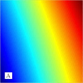
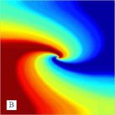
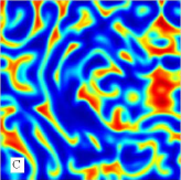
Figure 9: (Color online) Snapshots of contour pictures of the time evolution of the prey at different instants with the special initial condition and $S=0.6<S_{T}$. (A) 0 iteration; (B) 1000 iterations; (C) 400000 iterations. [Additional movie format available from the author]

In Ref. Medvinsky et al. (2002), the authors explained the field meaning by using aquatic community in the ocean (cf. Fig. 9). Our study shows that the spatially extended model (Eq. 12) has not only more complex dynamic patterns in the space, but also chaos patterns and spiral waves, so it may help us better understand the dynamics of an aquatic community in a real marine environment. It is also important to distinguish between “intrinsic” patterns, i.e., patterns arising due to trophic interactions like those considered above, and “forced” patterns induced by the inhomogeneity of the environment. The physical nature of the environmental heterogeneity, and thus the value of the dispersion of varying quantities and typical times and lengths, can be essentially different in different cases. Neuhauser and Pacala Neuhauser and Pacala (1999) formulated the Lotka-Volterra model as a spatial model. They found the striking result that the coexistence of patterns is actually harder to get in the spatial model than in the non-spatial one. One reason can be traced to how local interactions between individual members of the species are represented in the model. In this thesis, our results show that the ratio-dependent predator-prey model (Eq. 12) also represents rich spatial dynamics, such as chaos spiral patterns, stripelike patterns, spotted patterns, coexistence of both stripelike and spotted patterns, etc. It will be useful for studying the dynamic complexity of ecosystems.