Genotype-based Case-Control Analysis, Violation of Hardy-Weinberg Equilibrium, and Phase Diagrams

Abstract

We study in detail a particular statistical method in genetic case-control analysis, labeled “genotype-based association”, in which the two test results from assuming dominant and recessive model are combined in one optimal output. This method differs both from the allele-based association which artificially doubles the sample size, and the direct $\chi^{2}$ test on 3-by-2 contingency table which may overestimate the degree of freedom. We conclude that the comparative advantage (or disadvantage) of the genotype-based test over the allele-based test mainly depends on two parameters, the allele frequency difference $\delta$ and the Hardy-Weinberg disequilibrium coefficient difference $\delta_{\epsilon}$. Six different situations, called “phases”, characterized by the two $X^{2}$ test statistics in allele-based and genotype-based test, are well separated in the phase diagram parameterized by $\delta$ and $\delta_{\epsilon}$. For two major groups of phases, a single parameter $\theta=tan^{-1}(\delta/\delta_{\epsilon})$ is able to achieves an almost perfect phase separation. We also applied the analytic result to several types of disease models. It is shown that for dominant and additive models, genotype-based tests are favored over allele-based tests.

1 Introduction

Genetic association analysis is a major tool in mapping human disease genes[16, 7, 11]. A simple association study is the case-control analysis, in which individuals with and without disease are collected (roughly the equal number of sample per group for an optimal design), DNA samples extracted and genetic markers typed. The prototype of a genetic marker is the two-allele single-nucleotide-polymorphism (SNP)[4]. If the two alleles are $A$ and $a$, there three possible genotypes: $AA$, $Aa$, $aa$, consisting of the maternally-derived and paternally-derived copy of an allele. The three genotype frequencies are calculated in case (disease) and control (normal) group, and a strong contrast of the two sets of genotype frequencies can be used to indicate an association between that marker and the disease.

The statistical analysis in an association study seems to be simple – mostly the standard Pearson’s $\chi^{2}$ test in categorical analysis[1], there are nevertheless subtle differences among various approaches. Some people use the $2\times 3$ genotype count table to carry about test with $\chi^{2}$ distribution of $df=2$ degrees of freedom[6]. This method may overestimate the degree of freedom if the Hardy-Weinberg equilibrium holds true. Other people use the allele-based test, where each person contributes two allele counts, and the allele frequency is compared in a $2\times 2$ allele count table. This approach artificially doubles the sample sizes without a theoretical justification[17]. A third approach, what we called “genotype-based” case-control association analysis, remains faithful to the sample size, while does not overestimate the degrees of freedom.

A genotype-based analysis can be simply summarized here. Two Pearson’s $\chi^{2}$ tests are carried out on two $2\times 2$ count tables: the first is constructed by combining the $AA$ and $Aa$ genotype counts and keeping the $aa$ genotype column, and the second by combining the $Aa$ and $aa$ genotype counts. If the marker happens to be the disease gene and $A$ is the mutant allele ($a$ is the wild type allele), then the first table is consistent with a dominant disease model, whereas second a recessive disease model. The two $\chi^{2}$ tests lead to two $p$-values, and the smallest one (the more significant one) is chosen as the final test result.

Genotype-based analysis has been used in practice many times[20, 18, 9], without a particular name, and without a theoretical study. In this article, we will take a deeper look of the genotype-based analysis. We will show that the justification of using genotype-based tests is intrinsically related to the Hardy-Weinberg disequilibrium, but there are more than just a non-zero Hardy-Weinberg disequilibrium coefficient that is important.

The article is organized as follows: we first show that there is no advantage in using genotype-based test if there is no Hardy-Weinberg disequilibrium; we then examine the situation with Hardy-Weinberg disequilibrium, and use the two parameters, the allele frequency difference and the difference of two Hardy-Weinberg disequilibrium coefficients, to construct a phase diagram; the phase diagram is further simplified by using just one parameter; our analytic result is illustrated by a real example from the study of rheumatoid arthritis; we apply the formula to different models; and finally future works are discussed.

2 No advantage for genotype-based analysis if Hardy-Weinberg equilibrium holds true exactly

In an ideal situation, we assume $N$ case samples and $N$ control samples, and the $A$ allele frequency in case and control groups is $p_{1}$ and $p_{2}$ ($q_{1}=1-p_{1},q_{2}=1-p_{2}$). On average (or in the asymptotic limit), the allele and genotype counts are listed in Table 2 where the Hardy-Weinberg equilibrium (HWE) is assumed.

For a $\{N_{ij}\}$ ($i,j=1,2$) 2-by-2 contingency table, the Pearson’s (O-E)²/E (O for observed count, and E for expected count) test statistic is:

$$X^{2}=\frac{(N_{11}N_{22}-N_{12}N_{21})^{2}(N_{11}+N_{12}+N_{21}+N_{22})}{(N_{11}+N_{12})(N_{21}+N_{22})(N_{11}+N_{21})(N_{12}+N_{22})}$$ (1)

Using the table elements in Table 2, we can derive

$$X^{2}_{\rm allele} = \frac{(2N)^{4}(p_{1}q_{2}-p_{2}q_{1})^{2}4N}{(2N)^{4}(p_{1}+p_{2})(q_{1}+q_{2})}=\frac{4N(p_{1}-p_{2})^{2}}{(p_{1}+p_{2})(q_{1}+q_{2})}$$

$$X^{2}_{\rm dom} = \frac{N^{4}[(p_{1}^{2}+2p_{1}q_{1})q_{2}^{2}-(p_{2}^{2}+2p_{2}q_{2})q_{1}^{2}]^{2}2N}{N^{4}(p_{1}^{2}+2p_{1}q_{1}+p_{2}^{2}+2p_{2}q_{2})(q_{1}^{2}+q_{2}^{2})}=\frac{2N(p_{1}-p_{2})^{2}(q_{1}+q_{2})^{2}}{(2-q_{1}^{2}-q_{2}^{2})(q_{1}^{2}+q_{2}^{2})}$$

$$X^{2}_{\rm rec} = \frac{N^{4}[(q_{1}^{2}+2p_{1}q_{1})p_{2}^{2}-(q_{2}^{2}+2p_{2}q_{2})p_{1}^{2}]^{2}2N}{N^{4}(q_{1}^{2}+2p_{1}q_{1}+q_{2}^{2}+2p_{2}q_{2})(p_{1}^{2}+p_{2}^{2})}=\frac{2N(q_{1}-q_{2})^{2}(p_{1}+p_{2})^{2}}{(2-p_{1}^{2}-p_{2}^{2})(p_{1}^{2}+p_{2}^{2})}$$ (2)

To further simplify the notation, let’s denote $\delta\equiv p_{1}-p_{2}$ as the allele frequency difference, $\overline{p}\equiv(p_{1}+p_{2})/2$ as the averaged $A$ allele frequency across groups, and the averages of the squared terms $\overline{p^{2}}\equiv(p_{1}^{2}+p_{2}^{2})/2$ ($\overline{q}$ and $\overline{q^{2}}$ are defined similarly). Then Eq.(2) becomes:

$$X^{2}_{\rm allele} = \frac{N\delta^{2}}{\overline{p}\cdot\overline{q}},$$

$$X^{2}_{\rm dom} = \frac{2N\delta^{2}\overline{q}^{2}}{\overline{q^{2}}(1-\overline{q^{2}})},$$

$$X^{2}_{\rm rec} = \frac{2N\delta^{2}\overline{p}^{2}}{\overline{p^{2}}(1-\overline{p^{2}})}.$$ (3)

Since the genotype-based test is determined by the maximum value among $X^{2}_{\rm dom}$ and $X^{2}_{\rm rec}$, we would like to prove an inequality between $X^{2}_{\rm allele}$ and max($X^{2}_{\rm dom}$,$X^{2}_{\rm rec}$).

Count tables for genotype-based analysis under HWE $A$ $a$ $AA+Aa$ $aa$ $AA$ $AA+Aa$ allele count dominant model recessive model case 2 $Np_{1}$ 2 $Nq_{1}$ $N(p_{1}^{2}+2p_{1}q_{1})$ $Nq_{1}^{2}$ N$p_{1}^{2}$ N($2p_{1}q_{1}+q_{1}^{2}$) control 2 $Np_{2}$ 2 $Nq_{2}$ $N(p_{2}^{2}+2p_{2}q_{2})$ $Nq_{2}^{2}$ $Np_{2}^{2}$ $N(2p_{2}q_{2}+q_{2}^{2})$

Towards this aim, we first compare $X^{2}_{\rm allele}$ and $X^{2}_{\rm dom}$. Due to the following two inequalities:

$$\overline{q^{2}} = \frac{2q_{1}^{2}+2q_{2}^{2}}{4}\geq\frac{2q_{1}^{2}+2q_{2}^{2}-(q_{1}-q_{2})^{2}}{4}=\frac{(q_{1}+q_{2})^{2}}{4}=\overline{q}^{2}$$

$$2\overline{p}\cdot\overline{q} = 2\overline{q}-2\overline{q}^{2}=q_{1}+q_{2}-(q_{1}q_{2}+\overline{q^{2}})=1-\overline{q^{2}}-(1-q_{1})(1-q_{2})\leq 1-\overline{q^{2}},$$

we have

$$\frac{\overline{q^{2}}}{2\overline{p}\cdot\overline{q}}\geq\frac{\overline{q}^{2}}{1-\overline{q^{2}}},$$ (4)

which leads to $X^{2}_{\rm allele}\geq X^{2}_{\rm dom}$. The similar approach shows that $\overline{p^{2}}\geq\overline{p}^{2}$ and $2\overline{p}\cdot\overline{q}\leq 1-\overline{p^{2}}$, which leads to $X^{2}_{\rm allele}\geq X^{2}_{\rm rec}$.

With the proof that $X^{2}_{\rm allele}\geq\max(X^{2}_{\rm dom},X^{2}_{\rm rec})$, we have shown that allele-based $X^{2}$ ($p$-value) is always larger (smaller) than the genotype-based $X^{2}$ ($p$-value). In other words, if HWE holds exactly true, there is no need to carry out a genotype-based association analysis. To certain extend, this result is not surprising since allele-based test utlizes twice the number of samples as the genotype-based test, even though the latter has one advantage of testing multiple (two) disease models. Clearly, the increase in sample size more than compensates the advantage of testing multiple models, when HWE is true.

Count tables for genotype-based analysis under HWD $A$ $a$ $AA+Aa$ $aa$ $AA$ $AA+Aa$ allele count dominant model recessive model case 2 $Np_{1}$ 2 $Nq_{1}$ $N(p_{1}^{2}+2p_{1}q_{1}-\epsilon_{1})$ $N(q_{1}^{2}+\epsilon_{1})$ N($p_{1}^{2}+\epsilon_{1}$) N($2p_{1}q_{1}+q_{1}^{2}-\epsilon_{1}$) control 2 $Np_{2}$ 2 $Nq_{2}$ $N(p_{2}^{2}+2p_{2}q_{2}-\epsilon_{2})$ $N(q_{2}^{2}+\epsilon_{2})$ $N(p_{2}^{2}+\epsilon_{2})$ $N(2p_{2}q_{2}+q_{2}^{2}-\epsilon_{2})$

3 Adding violation of Hardy-Weinberg equilibrium

The result in the previous section actually does not disapprove the genotype-based association, since HWE in real data is often violated, even if it is not significantly violated. To characterize a realistic genotype count table, one more parameter besides the allele frequency is needed: the Hardy-Weinberg disequilibrium coefficient (HWDc)[19]. The HWDc $\epsilon$ is defined as[19] $\epsilon=p_{AA}-p_{A}^{2}=p_{aa}-p_{a}^{2}=-(p_{Aa}-2p_{a}p_{A})/2=p_{aa}p_{AA}-p_{Aa}^{2}/4$. For case and control groups, two HWDc’s are used $\epsilon_{1}$ and $\epsilon_{2}$. The three count tables under HWD are now parameterized in Table 2.

Applying the definition of $X^{2}$ in Eq.(1) to the count tables in Table 2 (note that the allele counts are not affected by HWD), we have

$$X^{2}_{\rm allele} = \frac{4N(p_{1}-p_{2})^{2}}{(p_{1}+p_{2})(q_{1}+q_{2})}$$

$$X^{2}_{\rm dom,HWD} = \frac{N^{4}[(p_{1}^{2}+2p_{1}q_{1}-\epsilon_{1})(q_{2}^{2}+\epsilon_{2})-(p_{2}^{2}+2p_{2}q_{2}-\epsilon_{2})(q_{1}^{2}+\epsilon_{1})]^{2}2N}{N^{4}(p_{1}^{2}+2p_{1}q_{1}+p_{2}^{2}+2p_{2}q_{2}-\epsilon_{1}-\epsilon_{2})(q_{1}^{2}+q_{2}^{2}+\epsilon_{1}+\epsilon_{2})}$$

$$= \frac{2N[(p_{1}-p_{2})(q_{1}+q_{2})-(\epsilon_{1}-\epsilon_{2})]^{2}}{(2-q_{1}^{2}-q_{2}^{2}-\epsilon_{1}-\epsilon_{2})(q_{1}^{2}+q_{2}^{2}+\epsilon_{1}+\epsilon_{2})}$$

$$X^{2}_{\rm rec,HWD} = \frac{N^{4}[(q_{1}^{2}+2p_{1}q_{1}-\epsilon_{1})(p_{2}^{2}+\epsilon_{2})-(q_{2}^{2}+2p_{2}q_{2}-\epsilon_{2})(p_{1}^{2}+\epsilon_{1})]^{2}2N}{N^{4}(q_{1}^{2}+2p_{1}q_{1}+q_{2}^{2}+2p_{2}q_{2}-\epsilon_{1}-\epsilon_{2})(p_{1}^{2}+p_{2}^{2}+\epsilon_{1}+\epsilon_{2})}$$ (5)

$$= \frac{2N[(q_{1}-q_{2})(p_{1}+p_{2})-(\epsilon_{1}-\epsilon_{2})]^{2}}{(2-p_{1}^{2}-p_{2}^{2}-\epsilon_{1}-\epsilon_{2})(p_{1}^{2}+p_{2}^{2}+\epsilon_{1}+\epsilon_{2})}$$

Again shorthand notations are introduced: $\delta_{\epsilon}\equiv\epsilon_{1}-\epsilon_{2}$, and $\overline{\epsilon}\equiv(\epsilon_{1}+\epsilon_{2})/2$. Eq.(3) is rewritten as

$$X^{2}_{\rm allele} = \frac{N\delta^{2}}{\overline{p}\cdot\overline{q}},$$

$$X^{2}_{\rm dom,HWD} = \frac{2N(\delta\overline{q}-\frac{\delta_{\epsilon}}{2})^{2}}{(\overline{q^{2}}+\overline{\epsilon})(1-\overline{q^{2}}-\overline{\epsilon})}$$

$$X^{2}_{\rm rec,HWD} = \frac{2N(\delta\overline{p}-\frac{\delta_{\epsilon}}{2})^{2}}{(\overline{p^{2}}+\overline{\epsilon})(1-\overline{p^{2}}-\overline{\epsilon})}$$ (6)

From Eq.(3), it is not clear whether $X^{2}_{\rm allele}$ is still larger than $X^{2}_{\rm dom,HWD}$ and $X^{2}_{\rm rec,HWD}$. Systematic scanning of the 4-parameter space ($p_{1},p_{2},\epsilon_{1},\epsilon_{2}$) would offer a solution, but the result cannot be displayed on a 2-dimensional space. In the following, we simplify the display of the “phase diagram” by using only two (or one) parameters.

4 Phase diagram with one and two parameters

The term “phase diagram” is borrowed from the field of statistical physics[12]. In a typical diagram used in statistical or chemical physics, phases (e.g. solid, liquid and gas) as well as phase boundaries (e.g. melting line) are displayed as a function of physical quantities such as temperature and pressure. Phase transition occurs at phase boundaries. For our topic, a phase indicates, for example, whether allele-based or genotype-based test leads to a higher $X^{2}$ value; or it can indicate whether or not the $X^{2}$ value leads to a statistically significant result (e.g. $p$-value $<$ 0.05). The quantities chosen to mimic temperature or pressure for our topic should highlight the phase separation and phase transitions.

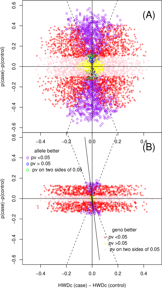
Figure 1: The phase diagram parameterized by $\delta_{\epsilon}=\epsilon_{1}-\epsilon_{2}$ (x-axis) and $\delta=p_{1}-p_{2}$ (y-axis), where $p$ is the allele frequency for $A$ and $\epsilon$ is the Hardy-Weinberg disequilibrium coefficient, determined by a numerical simulation. (A) 100 samples per group with 5000 replicates (5000 points in the plot); (B) 1000 samples per group with 5000 replicates. Six phases are marked: I. $p$-value for genotype-based test is smaller than that for allele-based test (and both $p$-values are smaller than 0.05) (red cross); II. similar to I, but both $p$-values are larger than 0.05 (yellow cross); III. similar to I, but one $p$-value is smaller than 0.05 and another larger than 0.05 (pink cross); IV. $p$-value for allele-based test is smaller than that for genotype-based test (and both $p$-values are smaller than 0.05) (purple circle); V. similar to IV, but both $p$-values are larger than 0.05 (blue circle); VI. similar to V, but one $p$-value is smaller than 0.05 and another larger than 0.05 (green circle). The two dashed lines have angle of 73.125^∘ and $-$73.125^∘, and the solid line has angle of 95.37${}^{c}irc$.

Eq.(3) provides us a hint that the allele frequency difference in two groups, $\delta$, and the HWDc difference, $\delta_{\epsilon}$, could be good quantities for phase separation. First of all, $\delta$ directly controls the magnitude of $X^{2}$, so it should separate “significant phases” from “insignificant phases”. Secondly, the relative magnitude and sign of $\delta$ and $\delta_{\epsilon}$ seems to control the difference between $X^{2}_{\rm allele}$ and $X^{2}_{\rm dom,HWD}$ or $X^{2}_{\rm rec,HWD}$, so it should be a good quantity to separate “favoring-allele-based-test phase” (when $X^{2}_{\rm allele}>\max(X^{2}_{\rm dom,HWD},X^{2}_{\rm rec,HWD})$) and “favoring-genotype-based-test phase” (when $X^{2}_{\rm allele}<\max(X^{2}_{\rm dom,HWD},X^{2}_{\rm rec,HWD})$).

We carried out the following simulation to construct the phase diagram: 5000 replicates of case-control datasets with 100 cases and 100 controls (in another simulation, the sample size is 1000 per group); For each replicate, the three genotypes are randomly chosen, then the allele frequency and Hardy-Weinberg disequilibrium coefficient were determined. Fig.1 shows the simulation result parameterized by $\delta_{\epsilon}$ (x-axis) and $\delta$ (y-axis). Six phases (labeled I-VI) are illustrated using 6 different colors, within the two larger categories:

• Favoring genotype-based tests (crosses in Fig.1)

  • I. $p$-values for both genotype- and allele-based tests are $<$ 0.05 (red)

  • II. $p$-values for both genotype- and allele-based tests are $>$ 0.05 (yellow)

  • III. $p$-value for genotype-based test is $<$ 0.05, that for allele-based test is $>$ 0.05 (pink)

• Favoring allele-based tests (circles in Fig.1)

  • IV. $p$-values for both genotype- and allele-based tests are $<$ 0.05 (purple)

  • V. $p$-values for both genotype- and allele-based tests are $>$ 0.05 (blue)

  • VI. $p$-value for allele-based test is $<$ 0.05, that for genotype-based test is $>$ 0.05 (green)

As can be seen from Fig.1, the two parameters, $\delta$ and $\delta_{\epsilon}$ does a pretty good job in separating six different phases, although minor overlap between phases occurs. The overall performance of $\delta$ and $\delta_{\epsilon}$ as phase parameters is satisfactory.

As expected, the magnitude of $p$-values is mainly controlled by the y-axis. Smaller allele frequency differences (smaller $\delta$’s) result in non-significant $p$-values, and significant results are located far away from the $\delta=0$ line. On the other hand, the $\delta_{\epsilon}$ mainly controls whether allele-based or genotype-based test is more significant. However, $\delta_{\epsilon}$ itself is not enough: it acts jointly with $\delta$ to achieve the phase separation: for genotype-based test to have a smaller $p$-value than the allele-based test and both are smaller than 0.05 (red points in Fig.1), $\delta_{\epsilon}$ tends to have the different sign as that of $\delta$.

The effect of sample size on the phase diagram can be examined by comparing Fig.1(A) and Fig.1(B). Phases II, III, V, VI all shrink in area simply because a larger sample size is more likely to lead to a $p$-value $<$ 0.05 replicate. The relative location of different phases in Fig.1 remains the same.

If we focus on the two major categories (phases I,II,III versus phases IV,V,VI), we notice that the phase boundaries are radiuses. The observation led to the following phase diagram by using a single parameter $\theta=tan^{-1}(y/x)=tan^{-1}(\delta/\delta_{\epsilon})$, i.e., the angle between a radius and the x-axis. To measure the relative advantage (disadvantage) of allele-based test over genotype-based test, we use the ratio of two $X^{2}$’s: $\lambda=X^{2}_{\rm allele}/\max(X^{2}_{\rm rec},X^{2}_{\rm dom})$. Fig.2 shows $\lambda$ as a function of $\theta$, using the simulation result in Fig.1 (100 samples per group and 1000 samples per group) and the same color code for six phases.

-90

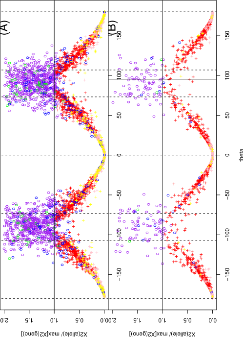
Figure 2: The $X^{2}$ ratio $\lambda=X^{2}_{\rm allele}/\max(X^{2}_{\rm rec},X^{2}_{\rm dom})$ as a function of the parameter $\theta=tan^{-1}(\delta/\delta_{\epsilon})$. The same color code for the six phases as used in Fig.1 is also used here. For phases that favor the genotype-based test, $\lambda<1$; for those favoring allele-based test, $\lambda>1$. (A) 100 samples per group with 5000 replicates; (B) 1000 samples per group with 5000 replicates. The vertical dashed lines correspond to angles of $\pm$ 73.125^∘ and $\pm$ 106.875^∘, and the solid vertical line corresponds to angle of 95.37${}^{c}irc$.

Fig.2 shows that within the range of $-13\pi/16<\theta<13\pi/16$ ($-73.125^{\circ}<\theta<73.125^{\circ}$, or $-3.2966<\delta/\delta_{\epsilon}<3.2966$), the genotype-based test is favored over the allele-based test. Overlap of phases still occurs in Fig.2, indicating the phase separation is not perfect. The allele-based test is much better than the genotype-based test when $\theta=\pi/2$ (90^∘). and the genotype-based test is much better than the allele-based test when $\theta=0$ (or $\delta=0$).

The sample size per group does not affect the phase boundary between the two major categories, though it does affect phases within a major category. This observation can be understood theoretically by the formula of $X^{2}$’s in Eq.(3): the relative magnitude between $X^{2}_{\rm allele}$ and $X^{2}_{\rm dom,HWD}$ or $X^{2}_{\rm rec,HWD}$ is independent of $N$ as it is canceled out.

Count tables of marker genotype for a SNP within the gene PTPN22 $TT$ $TC$ $CC$ total $p_{T}$ $\epsilon$ case 16 245 677 938 .147655 -0.004744 control 12 221 1168 1401 .087438 +0.000920 difference .060217 -.005664

5 Illustration by a real dataset

The genotype counts of a missense SNP in gene PTPN22 in Rheumatoid Arthritis samples and in control samples are listed in Table 4 (combining the “discovery” dataset and the “single sib” option in the “replication” dataset in Ref. begovich). Our formula predicts that $\theta=tan^{-1}(0.147655-0.087438)/(-0.004744-0.000920)=tan^{-1}(-0.060217/0.005664)=95.37^{\circ}$. This $\theta$ line is marked both in Fig.1 and Fig.2 in solid lines, and is within the phase where the allele-based test is preferred. Our calculation predicts that the allele-based test and genotype-based test should lead to similar result. Indeed, $X^{2}_{\rm allele}$=41.10, $X^{2}_{\rm dom,HWD}$=42.26, $X^{2}_{\rm rec,HWD}$=3.43, and allele-based and genotype-based test statistics are essentially the same.

6 Hardy-Weinberg disequilibrium in the patient population given a disease model

In the population of patients (case group), a SNP marker within the disease gene or in linkage disequilibrium with the disease usually violates the Hardy-Weinberg equilibrium. This fact has been used in the proposal of using HWD in case samples to map the disease gene[8]. The HWD coefficient in the case group can be calculated if the disease model is given[10], which is reproduced here. Assuming the penetrance for $AA,Aa,aa$ genotypes to be $f_{\rm AA},f_{\rm Aa},f_{\rm aa}$, the disease prevalence is $K=f_{\rm AA}p_{1}^{2}+f_{\rm Aa}2p_{1}q_{1}+f_{\rm aa}q_{1}^{2}$, and the genotype frequencies for the case group are (using the Bayes’ theorem):

$$p_{\rm AA,aff}=\frac{f_{\rm AA}p_{1}^{2}}{K},\hskip 14.45377ptp_{\rm Aa,aff}=\frac{f_{\rm Aa}2p_{1}q_{1}}{K},\hskip 14.45377ptp_{\rm aa,aff}=\frac{f_{\rm aa}q_{1}^{2}}{K}.$$ (7)

The HWD coefficient for the case group is then[10]:

$$\epsilon_{1}=p_{\rm AA,aff}\cdot p_{\rm aa,aff}-\frac{p_{\rm Aa,aff}^{2}}{4}=\left(\frac{p_{1}q_{1}}{K}\right)^{2}(f_{\rm AA}f_{\rm aa}-f_{\rm Aa}^{2}),$$ (8)

and the HWD coefficient for the control group is assumed to be zero ($\epsilon_{2}=0$).

If the disease model is multiplicative, i.e., $f_{\rm AA}/f_{\rm Aa}=f_{\rm Aa}/f_{\rm aa}$, there is no HWD in the case group, so HWD can not be used to map the disease gene. With $\delta_{\epsilon}=0-0=0$, from the result in Sec. 2, the allele-based test is favored over the genotype-based test. For dominant models, $f_{\rm AA}\approx f_{\rm Aa}=F$, and $\epsilon_{1}\propto F(f_{\rm aa}-F)$. Since we usually assume low phenocopy rate, i.e., $f_{\rm aa}\approx 0$, the HWDc $\epsilon_{1}\propto-F^{2}$ is negative. If the mutant allele $A$ is enriched in case samples ($\delta=p_{1}-p_{2}>0$), with the $\delta_{\epsilon}<0$ in dominant models, we conclude that genotype-based test is favored over allele-based tests. For recessive models, $f_{\rm Aa}\approx f_{\rm aa}\approx 0$, $\epsilon_{1}\propto 0$, so the allele-based test is better. For additive models, $f_{\rm Aa}=f_{\rm aa}+\Delta$, $f_{\rm AA}=f_{\rm aa}+2\Delta$, where $\Delta$ is the contribution to the penetrance by adding one copy of the mutant allele. The $\delta_{\epsilon}$ is equal to $\epsilon_{1}\propto(f_{\rm aa}+2\Delta)f_{\rm aa}-(f_{\rm aa}+\Delta)^{2}=-\Delta^{2}<0$. Thus genotype-based test is favored for additive disease models.

7 Discussion and future works

The main point of this article is that genotype-based test may take advantage of certain Hardy-Weinberg disequilibrium in case samples to overcome the advantage of larger sample sizes in allele-based tests. Another advantage of the genotype-based test is that it tests two models and picks the best one. This multiple testing might be corrected by multiplying the $p$-value by a factor of 2 (Bonferroni corrections), which was not done in this article. Whether correcting multiple testing or not is always under debate[14, 2, 15], but its effect on our problem is probably to shift the phase boundary slightly.

The $X^{2}$ test statistic calculation in this article was all carried out assuming equal number of samples in case and control group. Changing this assumption to unequal number of samples per group is not difficult, but its effect on the conclusion has not been examined.

Here we are addressing the type-I error of the test, the $p$-value, which is determined by the $X^{2}$ test statistic. For type-II error under alternative hypothesis, usually a non-central $\chi^{2}$ distribution could be used[13]. However, other alternatives to non-central $\chi^{2}$ distribution to calculate type-II error and the power have been proposed[5].

References

- [1] A. Agresti. Categorical Data Analysis (Wiley-Interscience, 2002).
- [2] M. Aickin. Other method for adjustment of multiple testing exists. BMJ, 318:127, 1999.
- [3] A.B. Begovich, et al., A missense single-nucleotide polymorphism in a gene encoding a protein tyrosine phosphatase (PTPN22) is associated with rheumatoid arthritis. Am. J. Human Genet., 75:330-337, 2004.
- [4] A.J. Brookes. The essence of SNPs. Gene, 234:177-186, 1999.
- [5] J. Bukszar, E.J. van den Oord. Accurate and efficient power calculations for tables in unmatched case-control designs. Stat. in Med., 25:2623-2646, 2006.
- [6] P.R. Burton, M.D. Tobin, J.K. Happer. Key concepts in genetic epidemiology. Lancet, 366:941-951, 2005.
- [7] H.J. Cordell, D.G. Clayton. Genetic association studies. Lancet, 366:1121-1131, 2005.
- [8] J.N. Feder, et al., A novel MHC class I-like gene is mutated in patients with hereditary haemochromatosis. Nature Genet., 13:399-408, 1996.
- [9] A.T. Lee, W. Li, A. Liew, C. Bombardier, M. Weisman, E.M. Massarotti, J. Kent, F. Wolfe, A.B. Begovich, P.K. Gregersen. The PTPN22 R620W polymorphism associates with RF positive rheumatoid arthritis in a dose-dependent manner but not with HLA-SE status. Genes and Immunity, 6:129-133, 2005.
- [10] W.C. Lee. Searching for disease-susceptibility loci by testing for Hardy-Weinberg disequilibrium in a gene bank of affected individuals. Am. J. Epidemiology, 158:397-400, 2003.
- [11] W. Li, edited, Bibliography: linkage disequilibrium analysis URL: http://www.nslij-genetics.org/ld/
- [12] E.M. Lifshitz, L.D. Landau. Statistical Physics: Course of Theoretical Physics, Volume 5, 3rd edition (Butterworth-Heinemann, 1980).
- [13] P.B. Patnaik. The non-central - and -Distribution and their applications. Biometrika, 36:202-232, 1949.
- [14] T.V. Perneger. What’s wrong with Bonferroni adjustments. BMJ, 316:1236-1238, 1998.
- [15] T.V. Perneger. Adjusting for multiple testing in studies is less important than other concerns. BMJ, 318:1288, 1999.
- [16] N. Risch, K. Merikangas. The future of genetic studies of complex human diseases. Science, 273:1516-1517, 1996.
- [17] P.D. Sasieni. From genotypes to genes: doubling the sample size. Biometrics, 53:1253-1261, 1997.
- [18] S. Tokuhiro, et al. An intronic SNP in a RUNX1 binding site of SLC22A4, encoding an organic cation transporter, is associated with rheumatoid arthritis. Nature Genet., 35:341-348, 2003.
- [19] B.S. Weir. Genetic Data Analysis II (Sinauer Associates, 1996).
- [20] R. Yamada, et al., Association between a single-nucleotide polymorphism in the promoter of the human interleukin-3 gene and rheumatoid arthritis in Japanese patients, and maximum-likelihood estimation of combinatorial effect that two genetic loci have on susceptibility to the disease. Am. J. Hum. Genet., 68:674-685, 2001.