Population models with singular equilibrium

Abstract

A class of models of biological population and communities with a singular equilibrium at the origin is analyzed; it is shown that these models can possess a dynamical regime of deterministic extinction, which is crucially important from the biological standpoint. This regime corresponds to the presence of a family of homoclinics to the origin, so-called elliptic sector. The complete analysis of possible topological structures in a neighborhood of the origin, as well as asymptotics to orbits tending to this point, is given. An algorithmic approach to analyze system behavior with parameter changes is presented. The developed methods and algorithm are applied to existing mathematical models of biological systems. In particular, we analyze a model of anticancer treatment with oncolytic viruses, a parasite-host interaction model, and a model of Chagas’ disease.

Keywords:

Non-analytic equilibrium; ratio-dependent response; pathogen transmission; elliptic sector; population extinction

1 Introduction

Mathematical models of predator-prey or parasite-host interaction and epidemiological models formulated as a system of ordinary differential equations (ODEs) share the same framework of modeling. The principles of these models, balance relations and decomposition of the rates of change into birth and death processes, which were applied since publications of Lotka-Volterra equations [1, 2] and ODE $SIR$-model of Kermack and McKendrick [3], have remained valid until today. Modifications were limited to replacing growth, death, and transmission rates by more complex functions, other types of functional responses, density-dependent mortality rates, or modes of pathogen transmission other than mass action kinetics.

In a number of cases different population models possess a distinct similar feature that complicates the analysis of the models; namely, a number of models are not defined at a singular point. Without loss of generality we can assume that this point is the origin $O(0,0)$. The models we consider in the present paper are formulated in such a way that this singularity is removable, for example, we can get rid of it by a time change. After the time change a topologically equivalent dynamical system in $\mathbb{R}_{+}^{2}$ is obtained, where $\mathbb{R}_{2}^{+}=\{(x,y)\colon x\geqslant 0,\,y\geqslant 0\}$, which is a natural state space for biologically motivated models. The origin $O(0,0)$ becomes a well defined equilibrium for this dynamical system. Sometimes, however, the usual approach by linearization fails to infer the structure of a neighborhood of $O(0,0)$ because the origin is a non-hyperbolic equilibrium for any parameter values (i.e., this point has both eigenvalues equal zero).

The main goal of the present paper is to describe completely the possible structures of a small neighborhood $\Omega$ of non-hyperbolic equilibrium point $O(0,0)$ in case of a particular class of differential equations that includes many biological models. We also present an algorithm to analyze such equations in $\Omega$ and apply this algorithm to a number of mathematical models. In particular, we show that the models under consideration can possess a dynamical regime of deterministic extinction, which is crucially important from the biological standpoint. This regime corresponds to the presence of a family of homoclinics to the origin, so-called elliptic sector. We note that the fine structure of the phase plane containing the elliptic sector was sometimes overlooked in the analysis of these models.

More specifically, we analyze non-hyperbolic equilibrium $O(0,0)$ of the following system of ODEs:

$$\begin{split}\frac{dx}{dt}&=P_{2}(x,y)+P^{*}(x,y),\\ \frac{dy}{dt}&=Q_{2}(x,y)+Q^{*}(x,y),\end{split}$$ (1)

where $P_{2}(x,y),\,Q_{2}(x,y)$ are homogeneous polynomials of the second order:

$$\begin{split}P_{2}(x,y)&=p_{2,1}x^{2}+p_{1,2}xy+p_{0,3}y^{2},\\ Q_{2}(x,y)&=q_{3,0}x^{2}+q_{2,1}xy+q_{1,2}y^{2},\end{split}$$

and $P^{*}(x,y)=O(|(x,y)|^{3}),\,Q^{*}(x,y)=O(|(x,y)|^{3})$, i.e., their Taylor series start with terms of order three or higher.

It is important to stress that many of the global properties of the models with the discussed peculiarity are determined by the properties of equilibrium $O(0,0)$, and, therefore, it is essential to know the exact structure of a neighborhood of this point and dependence of this structure on the model parameters.

We organize the paper as follows: Section 2 is devoted to examples of biologically motivated models, which, after a suitable time change, fall into the class of differential equations (1); in Section 3 we introduce the basic definitions and notations and state the main theorems that describe possible topological structures of the origin of system (1); here we also present an algorithm to study the structure of $\Omega$ of $O(0,0)$; in Section 4, using the algorithm from Section 3, we analyze some mathematical models, mainly those introduced in Section 2; Section 5 contains discussion and conclusions; finally, proofs of some mathematical statements are given in Appendix.

2 Motivation and background

Ratio-dependent models.

Deterministic predator-prey models can be written in the following ‘canonical’ general form:

$$\begin{split}\frac{dN}{dt}&=F(N)-g(N,P)P,\\ \frac{dP}{dt}&=eg(N,P)P-qP,\end{split}$$ (2)

where $N$ and $P$ are the densities (or biomasses) of prey and of predators, respectively. The production of prey in the absence of predators is described by the function $F(N)$, whereas $g(N,P)$ is the functional response (number of prey eaten per predator per unit time [4]). The constant $e$ is the trophic efficiency, and predators are assumed to die with a constant death rate $q$.

Many questions in predator-prey theory revolve around the expression that is used for the functional response $g(N,P)$. Much early work was only concerned with the way in which this function varies with prey density (e.g., the so-called Holling types $I,II,III$), ignoring the effect of predator density. For example, in the Lotka-Volterra models, where $g(N,P)=\alpha N$, or in models with the Holling type $II$ response [5], where $g(N,P)=\alpha N/(1+\alpha hN)$, the functional response is of the form $g=g(N)$ (termed ‘prey-dependent’ by Arditi and Ginzburg [6]), see also [7].

It was also recognized that the predator density could have a direct effect on the functional response. A number of such ‘predator-dependent’ models have been proposed, the most widely known are those of Hassel and Varley [8], DeAngelis et al. [9], or Beddington [10].

Arditi and Ginzburg suggested that the essential properties of predator dependence could be rendered by a simple form which was called ‘ratio-dependence’. The functional response is assumed to depend on the single variable $N/P$ rather than on the two separate variables $N$ and $P$. Under this supposition system (2) becomes

$$\begin{split}\frac{dN}{dt}&=F(N)-g(N/P)P,\\ \frac{dP}{dt}&=eg(N/P)P-qP.\end{split}$$ (3)

Discussion of the biological implications and relevance of the ratio-dependent models, together with their principal predictions, can be found in, e.g., [11, 12].

One particular model that received considerable attention is of the form

$$\begin{split}\frac{dN}{dt}&=rN\left(1-\frac{N}{K}\right)-\frac{\alpha NP}{P+\alpha hN}\,,\\ \frac{dP}{dt}&=e\frac{\alpha NP}{P+\alpha hN}-qP,\end{split}$$ (4)

where Michaelis-Menten or Holling type $II$ function

$$g(z)=\alpha z/(1+\alpha hz),\quad z=N/P$$

was used as the functional response.

The model (4) was studied in, e.g., [13, 14, 15, 16, 17, 18]. It was shown, by this particular example, that ratio-dependent models can display original dynamical properties that cannot be observed in two-dimensional prey-dependent models. For instance, the origin can be an equilibrium point simultaneously attractive and repelling, thus shedding light on ecological extinction. Coexistence of several dynamical regimes with the same set of parameters was also observed.

From the mathematical point of view, ratio-dependent predator-prey models raise delicate questions because the functional response is undefined at the origin $N=0,\,P=0$. As a consequence, the origin is a so-called non-analytical complicated equilibrium point [13].

We are only interested in the dynamics of system (3) in $\mathbb{R}_{2}^{+}=\{(N,P)\colon N\geqslant 0,\,P\geqslant 0\}$. Time scale change $dt\rightarrow(P+\alpha hN)dt$ for system (4) results in the system

$$\begin{split}\frac{dN}{dt}&=rN(1-N/K)(P+\alpha hN)-\alpha NP,\\ \frac{dP}{dt}&=e\alpha NP-qP(P+\alpha hN).\end{split}$$ (5)

The system (5) is well defined at $O(0,0)$, however, the Jacobian matrix at $O(0,0)$ is a zero matrix, i.e., $O(0,0)$ is a non-hyperbolic equilibrium of (5). Obviously, model (5) belongs to the class of ODEs (1).

Frequency-dependent pathogen transmission in a population of variable size.

Transmission is the key process in a host-pathogen interaction. In most early models transmission was assumed to occur through the law of mass-action. For example, in the classical model of two differential equations, formulated as a particular case of the general model of Kermack and McKendrick in their pioneer work [3], the transmission function takes the form $\beta SI$. Here $S$ is the density of susceptible individuals, $I$ is the density of infective individuals, and $\beta$ is the transmission coefficient. Note that, for mass action, the contacts per unit time per individual rise linear with the population density $N=S+I$ (careful elaboration on the models of contact process can be found in [19]).

At the other extreme, the contact rate might be independent of host density. Assuming that susceptible and infective were randomly mixed, this would lead to transmission following $\beta SI/N=\beta SI/(S+I)$. This mode of transmission is often called ‘frequency-dependent’ or ‘density-independent’ transmission [20]. It is often assumed in models of sexually transmitted diseases because the number of sexual partners of an individual usually depends on the mating system of the species and is weakly related to host density [21].

We note here that the distinction between these two modes of transmission is not crucially important for many problems in human diseases, because most pathogens cause little mortality and the total population size remains more or less constant [22].

Even if some demography processes are taken into account many epidemiological models are formulated so that the infectious disease spreads in a population that has a fixed size $N=\textrm{const}$ with balancing inflows and outflows due to birth or death or migration, see, e.g., [23, 22]. However, if the population growth or decrease is significant (it might be the case on long periods of time, e.g., for diseases transmitted vertically) or the disease causes enough death to influence the population size, then it is not reasonable to assume that the population size is constant. In this case the difference between the mass action transmission and the frequency-dependent transmission becomes profound [25, 24]. It is worth noting that the frequency-dependent transmission is considered to be more realistic for most human diseases [22].

Due to the particular form of the transmission function, $\beta SI/(S+I)$, the origin $S=0,\,I=0$ becomes undefined in models where host extinction is a possibility, and the properties of the origin crucially affect the global dynamics of the system.

As an example of such models, we rewrite a model of Chagas’ disease from [23, 26] that takes the form

$$\begin{split}\frac{dS}{dt}&=(b-r-v)S+(b_{1}(1-q)+c)I-\beta\frac{SI}{S+I}\,,\\ \frac{dI}{dt}&=(b_{1}q-r_{1}-c)I+vS+\beta\frac{SI}{S+I}\,,\end{split}$$ (6)

where $b,\,b_{1},\,r,\,r_{1},\,c,\,q$, respectively, denote the birth rates of susceptible and infective individuals, their death rates, the cure rate and the probability of vertical transmission; $v$ is the transmission rate of disease by a vector. From (6) we have

$$\frac{d}{dt}(S+I)=(b-r)S+(b_{1}-r_{1})I,$$

and the total population could be either increasing or decreasing.

A usual way to analyze models like (6) is to perform the change of variables $x=S/(S+I),\,y=I/(S+I)$. After this and using the fact that $x+y=1$, it is often straightforward to obtain the analysis of the system in coordinates $x,\,y$, simultaneously keeping track of the asymptotic behavior of the total population size $N$ [23, 25, 24]. However, after this transformation some of the information concerning initial variables $S$ and $I$ can be lost. For example, in variables $x$ and $y$ it is difficult to see that the origin can be simultaneously attractive and repelling, and deterministic extinction of the total population can be accompanied by an initial growth of the susceptible subpopulation (see Section 4, Example 3).

Though mathematical models of pathogen transmission with function $\beta SI/N$ were extensively studied for years, the first case study, to our knowledge, that focuses on the possibility of deterministic extinction of host population was considered in [27]. A careful analysis of a more general model was presented in [28].

As an example, let us state the model of host-parasite interaction from [29]. This model allows for host extinction and, formulated through the basic birth and death processes, has the form

$$\begin{split}\frac{dS}{dt}&=a(S+I)-a(1-\theta)I-cS(S+I)-(d+m)S-\beta\frac{SI}{S+I}\,,\\ \frac{dI}{dt}&=-(d+\alpha)I-cI(S+I)+\beta\frac{SI}{S+I}\,,\end{split}$$ (7)

where $a,\,c,\,d,\,m,\,\alpha$ are nonnegative parameters, and $0\leqslant\theta\leqslant 1$. Model (7) was reduced to a Gause-type system by means of one blow-up transformation $(S,I)\rightarrow(u,I),\,u=S/I$. We show (Section 4, Example 2) that using this transformation is not enough to obtain a complete qualitative picture of a neighborhood of $O(0,0)$.

Systems (6) and (7) can be transformed into polynomial systems with a non-hyperbolic equilibrium at the origin by the time change $dt\rightarrow(S+I)dt$, and the resulting systems of ODEs are in the class (1).

It is worth mentioning that if the pathogen transmission follows mass action kinetics, but $S$ and $I$ denote numbers and not densities, and the total population density (here we speak of local spatial density) remains constant, one has to use $\beta SI/(S+I)$ expression to model transmission of disease [30].

Other models.

We by no means gave a full list of models analysis of which requires the knowledge of the structure of $\Omega$ of undefined equilibrium $O(0,0)$ and which can be reduced to (1). Similar models appear in many other areas of mathematical modeling in biology. Some mathematical models of interaction between populations of cells with a virus population can also be formulated in the form (1); e.g., one such model was applied to simulate anticancer therapy with oncolytic viruses [31] (see Section 4, Example 1). It was shown that the model possesses dynamical regimes that lead to elimination of cancer cells (a phenomenon known from clinical trials). Recently it was suggested that immune system response is more consistent with empirical data if it is considered to be ratio-dependent, see, e.g., [32].

3 Non-hyperbolic equilibrium of system (1) and structures of its neighborhood

3.1 Preliminaries

Let $O(0,0)$ be an isolated singular point of the vector field

$$J(x,y)=P(x,y)\frac{\partial}{\partial x}+Q(x,y)\frac{\partial}{\partial y}$$ (8)

and, correspondingly, an isolated equilibrium of the system of ODEs

$$\frac{dx}{dt}=P(x,y),\quad\frac{dy}{dt}=Q(x,y).$$ (9)

Here

$$P(x,y)=P_{n}(x,y)+P^{*}(x,y),\quad Q(x,y)=Q_{n}(x,y)+Q^{*}(x,y),$$

where $P_{n}(x,y),\,Q_{n}(x,y)$ are homogeneous polynomials of the $n$-th order:

$$\begin{split}P_{n}(x,y)&=p_{n,1}x^{n}+p_{n-1,2}x^{n-1}y+\ldots+p_{0,n+1}y^{n},\\ Q_{n}(x,y)&=q_{n+1,0}x^{n}+q_{n,1}x^{n-1}y+\ldots+q_{1,n}y^{n},\end{split}$$

and $P^{*}(x,y)=O(|(x,y)|^{n+1}),\,Q^{*}(x,y)=O(|(x,y)|^{n+1})$.

It is well known (e.g., [33]) that point $O(0,0)$ can be either monodromic (i.e., a focus or a center) or all orbits of system (9), tending to the origin for $t\to\infty$ or $t\to-\infty$ (we shall call such orbits as $O$-orbits), approach the origin along characteristic directions. The latter means that any $O$-orbit has definite direction $\theta$ so that $\arctan(y(t)/x(t))\to\theta$ for $t\to\infty$ or $t\to-\infty$. We note that the number of characteristic directions is finite in the generic case. Hereafter we refer to Andronov et al. [33] for a number of results and notations used, but restate some of the results in the form convenient for our exposition.

Following the results from Ch.VIII Sec. 17 of [33] we can state that any small enough neighborhood $\Omega$ of an isolated equilibrium point of an analytic system can be partitioned by $O$-orbits with characteristic directions into open regions, called sectors. These sectors can be classified into three types: parabolic sectors, hyperbolic sectors, and elliptic sectors, respectively; we shall call them the Brouwer sectors. The Brouwer sectors are described in the following figure (Fig. 1) and their definitions are given, e.g., in [33]. Note that the topological equivalence of a sector to one of the sectors in Fig. 1 need not preserve the directions of the flow.

Figure 1: The Brouwer sectors. (a) A parabolic sector ; (b) a hyperbolic sector ; (c) an elliptic sector

More exactly, the next statement is valid.

Theorem 1.

There exists a neighborhood $\Omega$ of a non-monodromic singular point of $C^{\infty}$-vector field, such that any neighborhood $\tilde{\Omega}\subset\Omega$ that contains this singular point can be partitioned into a finite number of sectors of parabolic, hyperbolic and elliptic types. The number, types and the cyclic order of a position of these sectors hold with decreasing of the size of neighborhood $\tilde{\Omega}$.

For $n=1$ we have

$$P_{1}(x,y)=p_{11}x+p_{02}y\,,\quad Q_{1}(x,y)=q_{20}x+q_{11}y\,.$$

Equilibrium $O(0,0)$ of (9) with $n=1$ is hyperbolic if $D=p_{11}q_{11}+p_{02}q_{20}\neq 0$ and $Tr=p_{11}+q_{11}\neq 0$ for $D>0$. Point $O(0,0)$ has $O$-orbits with characteristic directions if $Tr^{2}-4D\geqslant 0$. If the last condition holds and additionally $D\neq 0$ then $O(0,0)$ is a saddle whose neighborhood $\Omega$ contains four hyperbolic sectors, or $O(0,0)$ is a node whose neighborhood $\Omega$ contains only parabolic sectors. In general, the type of the origin of system (9) in the case $n=1$ is determined by the calculation of eigenvalues, and there is a simple algorithm to infer the structure of a small neighborhood of this point.

For $n\geqslant 2$ the situation is more complicated. Equilibrium point $O(0,0)$ is not hyperbolic (both eigenvalues are zero). The following problem is of principal interest: to describe all possible topological structures of a small neighborhood $\Omega$ of $O(0,0)$ and asymptotic behavior of orbits with variation of the system coefficients. In the present work we solve this problem in an important case $n=2$ under some additional assumptions on (9).

The problem of finding and describing the sequence of the Brouwer sectors that constitute $\Omega$, as well as asymptotics of $O$-orbits, was studied in a number of works [34, 35, 36, 37, 38, 39]. The main attention was paid to constructing algorithms of analysis of a non-hyperbolic equilibrium with the parameter values fixed. The general blow-up method, developed in [38, 39, 36] for so-called ‘system with a fixed Newton diagram’, allowed to describe topological structures of $\Omega$ and compute asymptotics of $O$-orbits close to the singular point. Below we apply the developed methods to system (9) with $n=2$ and present an approach to analyze the behavior of (9) with parameter changes.

3.2 Basic theorems

Let us consider system (9) with $n=2$ in neighborhood $\Omega$ of an isolated equilibrium $O(0,0)$, and let

$$F(x,y)=xQ_{n}(x,y)-yP_{n}(x,y).$$

Definition 1.

We shall call vector field (8) (and the corresponding system of ODEs (9)) non-degenerate in $\Omega$ if

$$\begin{split}(C1)\qquad&\mbox{polynomials $P_{n}(x,y),\,Q_{n}(x,y)$ have no common factors of the form}\\ &\mbox{$ax+by$, where at least one the constants $a,\,b$ is non-zero;}\\ (C2)\qquad&\mbox{polynomial $F(x,y)$ has no factors of the form $(ax+by)^{k}$, where $k>1$.}\end{split}$$

The coefficients of polynomials $P_{2}(x,y)$ and $Q_{2}(x,y)$ can be considered as the system parameters, and the parameter space is divided into domains of topologically equivalent behavior. The main results of our analysis show that each parameter domain corresponds to one of the following four types of phase portraits (Fig. 2).

Theorem 2.

Let system (9) with $n=2$ be non-degenerate. The positional relationship of the Brouwer sectors in $\Omega$ can be of four topologically non-equivalent cases:

(i) six hyperbolic sectors (Fig. 2a);

(ii) two hyperbolic sectors separated by two parabolic sectors such that one of the parabolic sectors is attracting (in a sense that $O$-orbits tend to $O(0,0)$ for $t\to\infty$) and another is repelling ($O$-orbits tend to $O(0,0)$ for $t\to-\infty$) (Fig. 2b);

(iii) two hyperbolic sectors (Fig. 2c);

(iv) two elliptic sectors separated by two parabolic sectors such that one of the parabolic sectors is attracting and another is repelling (Fig. 2d).

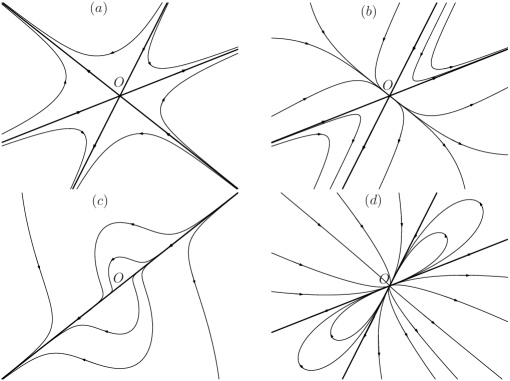
Figure 2: Four possible types of the topological structure of $\Omega$ of $O(0,0)$ for system (9) with $n=2$

Remarks to Theorem 2.

1. In the case considered there are always $O$-orbits with characteristic directions.

2. The boundaries between the parameter domains are given by violations of conditions $(C1)$ and $(C2)$. Violation of $(C1)$ leads to the presence of a straight line, passing through the origin, of non-isolated equilibrium points of (9), violation of $(C2)$ may lead to disappearance of characteristic directions.

3. The topological equivalence to one of the presented in Fig. 2 cases need not preserve the directions of the flow.

To describe possible asymptotics of $O$-orbits of system (9) we require the following condition:

$$(C3)\qquad P_{n}(0,y)\equiv 0\Rightarrow P^{*}(0,y)\equiv 0,\quad Q_{n}(x,0)\equiv 0\Rightarrow Q^{*}(x,0)\equiv 0.$$

Recall that curve $y=f(x)$, $f(0)=0$ has an exponential asymptotic with positive power $\rho$ and non-zero coefficient $k$ if

$$f(x)=kx^{\rho}(1+o(1)),\quad k\neq 0,\,\rho>0.$$ (10)

Theorem 3.

Let system (9) be non-degenerate. Then

(i) An $O$-orbit with a characteristic direction has asymptotic (10) with $\rho=1$ if and only if polynomial $F(1,u)$ has a root $\hat{u}=k\neq 0$; if $P_{2}(0,y)Q_{2}(x,0)\neq 0$ then system (9) has no $O$-orbits with other asymptotics;

(ii) If $Q_{2}(x,0)\equiv 0$ and $(C3)$ holds then system (9) has trivial orbits $y=0$ for $x>0$ and $x<0$; if additionally $\beta=q_{2,1}/p_{2,1}>1$ then (9) has a family of exponential asymptotics (10) with $\rho=\beta$, and $k\neq 0$ is an arbitrary constant;

(iii) If $P_{2}(0,y)\equiv 0$ and $(C3)$ holds then system (9) has trivial orbits $x=0$ for $y>0$ and $y<0$; if additionally $\beta=p_{1,2}/q_{1,2}>1$ then (9) has a family of exponential asymptotics (10) with $\rho=1/\beta$, and $k\neq 0$ is an arbitrary constant.

The proofs of Theorems 2 and 3 are given in Appendix.

3.3 An algorithmic approach to the analysis of the structure of the origin of system (1)

The results from the previous section show what can be expected in neighborhood $\Omega$ of the origin of system (1). Here we summarize a practical recipe to construct a phase-parameter portrait of (1), i.e., we show how to analyze a particular system. The presented algorithm follows directly from the proof of Theorem 2 (see Appendix).

Due to the homogeneous form of system (1) the analysis of an isolated equilibrium $O(0,0)$ can be formulated in terms of functions depending on one variable. Let $F(x,y)=xQ_{2}(x,y)-yP_{2}(x,y)$. We need to consider two pairs of polynomials

$$\textrm{(i)}\qquad P_{2}(1,u),\quad F_{1}(u)=F(1,u),$$

and

$$\textrm{(ii)}\qquad Q_{2}(v,1),\quad F_{2}(v)=-F(v,1).$$

The conditions of non-degeneracy $(C1)$ and $(C2)$ take the form:

$(C1^{\prime})$ The pair of polynomials $P_{2}(1,u),\,Q_{2}(1,u)$, as well as the pair of polynomials $P_{2}(v,1),\,Q_{2}(v,1)$, have no common roots;

$(C2^{\prime})$ The polynomials $F_{1}(u)$ and $F_{2}(v)$ have no multiple roots.

The analysis relies on finding the roots of $F_{1}(u)$ and $F_{2}(v)$. There can be five different cases, where we list only the roots that are necessary for the subsequent calculations:

(i) $F_{1}(u)$ has three real roots $\hat{u}_{i}$, $i=1,2,3$;

(ii) $F_{1}(u)$ has two real roots $\hat{u}_{i}\neq 0$, $i=1,2,$ and zero is a root of $F_{2}(v)$;

(iii) $F_{1}(u)$ has two real roots $\hat{u}_{1}=0,\,\hat{u}_{2}\neq 0$, and zero is a root of $F_{2}(v)$;

(iv) $F_{1}(u)$ has one real root;

(v) $F_{1}(u)$ has no real roots, and zero is a root of $F_{2}(v)$.

The lines $y=\hat{u}_{i}x$ and, if zero is a root of $F_{2}(v)$, $x=0$ divide $\Omega$ of $O(0,0)$ into six (cases (i)-(iii)) or two (cases (iv)-(v)) sectors with six or two branches. These sectors can be of a hyperbolic, elliptic, or parabolic type. Each line consists of two branches divided by the point $O(0,0)$.

We introduce the following notations. For the branches of lines $y=\hat{u}_{i}x$ we consider

$$\lambda_{1}^{u}(\hat{u}_{i})=P_{2}(1,\hat{u}_{i}),\quad\lambda_{2}^{u}(\hat{u}_{i})=F_{1}^{\prime}(\hat{u}_{i}),$$

for the branches of line $x=\hat{v}=0$ we consider

$$\lambda_{1}^{v}(\hat{v})=Q_{2}(\hat{v},1),\quad\lambda_{2}^{v}(\hat{v})=F_{2}^{\prime}(\hat{v}).$$

Note that we need to use functions $F_{2}(v)$ and $Q_{2}(v,1)$ only in cases (ii), (iii) and (v).

We shall call numbers $\lambda_{1}^{u},\,\lambda_{2}^{u},\,\lambda_{1}^{v}$ and $\lambda_{2}^{v}$ the branch characteristics.

Definition 2.

We shall call a branch of a sector in the phase space $(x,y)$ of system (1) hyperbolic if the inequality $\lambda_{1}^{u}\lambda_{2}^{u}<0$ (or $\lambda_{1}^{v}\lambda_{2}^{v}<0$) holds, and parabolic if $\lambda_{1}^{u}\lambda_{2}^{u}>0$ (or $\lambda_{1}^{v}\lambda_{2}^{v}>0$) holds, where $\lambda_{1}^{u},\,\lambda_{2}^{u}$ (or $\lambda_{1}^{v},\,\lambda_{2}^{v}$) the branch characteristics.

Let $V$ be a sector in the state space of system (1) with a vertex at $O(0,0)$ composed by branches of the lines $y=\hat{u}_{1}x$ and $y=\hat{u}_{2}x$ (or one of the lines can be $x=0$), and $V_{\Omega}=V\bigcap\Omega$. The following proposition, proved in Appendix, holds.

Proposition 1.

$V_{\Omega}$ contains

(i) a hyperbolic sector if both of its branches are hyperbolic (Fig. 3a);

(ii) an elliptic sector if both of its branches are parabolic (Fig. 3b);

(iii) a parabolic sector (or its part) if one of the branches is hyperbolic and another is parabolic (Fig. 3c).

Figure 3: Placing of the Brouwer sectors depending on the type of the sector branches ($h$ – hyperbolic branch, $p$ – parabolic branch)

The direction of the phase flow on the sector branches is determined by the sign of $\lambda_{1}$. If $\lambda_{1}^{u}(\hat{u}_{i})<0$ then the phase flow goes to $O(0,0)$ for $x>0$ and from $O(0,0)$ for $x<0$ (see, e.g., the line $y=\hat{u}_{1}x$ in Fig. 3a); if $\lambda_{1}^{u}(\hat{u}_{i})>0$ then the phase flow goes from $O(0,0)$ for $x>0$ and to $O(0,0)$ for $x<0$ (the line $y=\hat{u}_{2}x$ in Fig. 3a). If $\lambda_{1}^{v}(0)<0$ then the phase flow goes to $O(0,0)$ for $y>0$ and from $O(0,0)$ for $y<0$; if $\lambda_{1}^{v}(0)>0$ then the phase flow goes from $O(0,0)$ for $y>0$ and to $O(0,0)$ for $y<0$.

The conditions that determine the boundaries of topologically non-equivalent domains in the parameter space now can be reformulated in terms of the branch characteristics. Namely,

$$\lambda_{1}^{u}(\hat{u}_{i})\lambda_{2}^{u}(\hat{u}_{i})=0$$

and, if 0 is a root of $F_{2}(v)$,

$$\lambda_{1}^{v}(0)\lambda_{2}^{v}(0)=0.$$

These conditions are more convenient for most practical purposes.

4 Examples

In this section we give a number of examples of analysis of the complicated non-analytical equilibrium point in biological models. Mainly we restrict our attention to $\mathbb{R}_{+}^{2}$, but emphasize that in some cases it is necessary to analyze not only the behavior of the state variables in $\mathbb{R}_{+}^{2}$ but also the behavior in adjacent areas.

Example 1.

(Mathematical model of anticancer treatment with oncolytic viruses) Oncolytic viruses that specifically target tumor cells are promising new therapeutic agents [40]. The interaction between an oncolytic virus and tumor cells is highly complex and nonlinear. Hence, to precisely define the conditions that are required for successful therapy by this approach, mathematical models are needed. Our model [31] was formulated through the incorporation of frequency-dependent mode of virus transmission into the model of Wodarz [41]. The model, which considers two types of tumor cells growing in logistic fashion, has the following form (non-dimensional variables and parameters are used):

$$\begin{split}\frac{dx}{dt}&=x(1-(x+y))-\beta\frac{xy}{x+y}\,,\\ \frac{dy}{dt}&=\gamma y(1-(x+y))+\beta\frac{xy}{x+y}-\delta y.\end{split}$$ (11)

Here $x,\,y$ are (scaled) sizes of non-infected and infected tumor cell populations, respectively; $\gamma,\,\beta,\,\delta>0$ are non-dimensional parameters ($\beta$ takes stock of the transmission rate, and $\delta$ describes the virus cytotoxicity).

After the time change $dt\to(x+y)dt$ we obtain the system of ODEs in the form (1). We have

$$P_{2}(x,y)=x^{2}+(1-\beta)xy,\quad Q_{2}(x,y)=(\gamma-\delta+\beta)xy+(\gamma-\delta)y^{2}.$$

The polynomial

$$F_{1}(u)=Q_{2}(1,u)-uP_{2}(1,u)=(\gamma-\delta+\beta-1)u(u+1),$$

if $\gamma-\delta+\beta\neq 1$, has two roots $\hat{u}_{1}=0$ and $\hat{u}_{2}=-1$. Polynomial $F_{2}(v)$ also has two roots, one of which $\hat{v}=0$ (another one is $\hat{v}_{2}=1/\hat{u}_{2}$ and we do not need to consider it). $\mathbb{R}_{+}^{2}$ is confined by the branches of the lines $y=\hat{u}_{1}x=0$ and $x=\hat{v}=0$. This means that the root $\hat{u}_{2}$ is redundant for our analysis as far as we are concerned with the system behavior in $\mathbb{R}_{+}^{2}$. The branch characteristics are

$$\lambda_{1}^{u}(0)=1,\quad\lambda_{2}^{u}(0)=\gamma-\delta+\beta-1,$$

and

$$\lambda_{1}^{v}(0)=\gamma-\delta,\quad\lambda_{2}^{v}(0)=-\lambda_{2}^{u}(0).$$

Analyzing the sign of these expressions allows us to completely describe a small neighborhood of $O(0,0)$ (Fig. 4 and the following theorem).

Figure 4: Phase-parameter portrait of a neighborhood of the origin of system (11) given as a cut of positive parameter space for an arbitrary fixed value of $\gamma>0$. The bifurcation boundaries are $\alpha_{1}=\{(\delta,\gamma)\colon\delta=\gamma\}$, and $\alpha_{2}=\{(\delta,\gamma)\colon\beta=\delta+1-\gamma\}$ ($h$ – hyperbolic branch, $p$ – parabolic branch)

Theorem 4.

For different positive values of parameters $\delta,\,\beta$, and $\gamma$ there exist three types of topologically different structures of the neighborhood $\Omega_{+}=\Omega\bigcap\mathbb{R}_{+}^{2}$ of point $O(0,0)$ (and, correspondingly, three topologically different phase portraits of system (11)):

(i) a repelling parabolic sector (domain $I$ in Fig. 4) for the parameter values $\delta<\gamma$. The phase curves of the system that tend to $O(0,0)$ are of the form

$$y=Cx^{\gamma+\delta-\beta}(1+o(1)),$$ (12)

if $\beta>\delta+1-\gamma$, and

$$y=Cx^{(\gamma-\delta)/(1-\beta)}(1+o(1)),$$ (13)

if $\beta<\delta+1-\gamma$; here $C\neq 0$ is an arbitrary constant;

(ii) an elliptic sector (domain $II$ in Fig. 4) composed by trajectories tending to $O(0,0)$ as $t\to\infty$ (with asymptotics given by (13)), as well as with $t\to-\infty$ (with asymptotics given by (12)) if $\delta>\gamma$ and $\beta>\delta+1-\gamma$;

(iii) a saddle sector (domain $III$ in Fig. 4) for the parameter values $\delta>\gamma$ and $\beta<\delta+1-\gamma$.

Remark to Theorem 4. Note that only one of two possible arrangements of the sector branches is shown in domain $I$ of Fig. 4. It is possible that the branch $x=0,\,y>0$ may be parabolic, and the branch $y=0,\,x>0$ may be hyperbolic. In both cases, though, we obtain that $O(0,0)$ is a repelling node, and $\Omega_{+}$ contains a parabolic sector.

The most beneficial domain of parameter values is domain $II$ in Fig. 4 (an elliptic sector). This domain corresponds to the total elimination of both cell populations (infected and uninfected) regardless of the initial conditions (this dynamical regime is observed in experimental studies, e.g., [42]). However, on its way to extinction, the overall tumor size $x+y$ can reach rather high values (which, with the parameters fixed, crucially depend on the initial conditions). This indicates that we must not only identify the conditions that favor tumor elimination, but also develop the optimal strategy to infect the initial tumor. In the framework of the considered model this can be done using the information on asymptotics (12) and (13) (see [31]).

Example 2.

(Parasite-host interaction model) Hwang and Kuang [29] formulated a host-parasite model allowing for host extinction. The model, which is a non-dimensional version of (7), is of the form

$$\begin{split}\frac{dx}{dt}&=x+y-(1-\theta)y-x(x+y)-\delta x-s\frac{xy}{x+y}\,,\\ \frac{dy}{dt}&=-(\delta+r)y-y(x+y)+s\frac{xy}{x+y}\,,\end{split}$$ (14)

where all parameters are non-negative, and $0\leqslant\theta\leqslant 1$. Solutions of (14) are considered in $\mathbb{R}^{2}_{+}$. Using the transformation $v=x/y$, Hwang and Kuang reduced model (14) to a Gause-type system which was completely studied.

After the time change $dt\to(x+y)dt$ we obtain

$$\begin{split}P_{2}(x,y)&=(1-\delta)x^{2}+(1-\delta-s+\theta)xy+\theta y^{2},\\ Q_{2}(x,y)&=(s-\delta-r)xy-(\delta+r)y^{2},\\ F_{1}(u)&=\left(-r+s-1\right)u+\left(-r-1+s-\theta\right){u}^{2}-\theta\,{u}^{3}.\end{split}$$

The polynomial $F_{1}(u)$ has three roots

$$\hat{u}_{1}=0,\quad\hat{u}_{2}=-1,\quad\hat{u}_{3}=(s-r-1)/\theta,$$

if $\hat{u}_{3}\neq 0,\,-1$ (case (i) in Section 3.3).

We note that if $\delta>1$ then, from (14), $\frac{d}{dt}(x+y)<0$ follows. Thus, we shall consider only the case when $0<\delta<1$.

The state space $\mathbb{R}_{+}^{2}$ may be contained in two sectors, so in this case we need to calculate the branch characteristics for the branches of three lines $y=\hat{u}_{i}x$. We obtain

$$\lambda_{1}^{u}(\hat{u}_{1})=1-\delta,\quad\lambda_{2}^{u}(\hat{u}_{1})=s-r-1,\quad\lambda_{1}^{u}(\hat{u}_{2})=s,\quad\lambda_{2}^{u}(\hat{u}_{2})=-(s-r-1+\theta),$$

and

$$\lambda_{1}^{u}(\hat{u}_{3})=-(\delta+r)A+s,\quad\lambda_{2}^{u}(\hat{u}_{3})=-(s-r-1)A,$$

where $A=(s-r-1)/\theta+1$.

Using $\lambda_{2}^{u}(\hat{u}_{1})=0$ and $\lambda_{1}^{u}(\hat{u}_{3})=0$ as bifurcation curves we can draw the complete parameter portrait in $\Omega_{+}=\Omega\bigcap\mathbb{R}_{+}^{2}$ of the origin (Fig. 5).

Figure 5: Phase-parameter portrait of a neighborhood of the origin of system (14) given as a cut of positive parameter space for arbitrary fixed values of $0<\theta<1$ and $0<\delta<1$. The bifurcation boundaries are $\alpha_{1}\colon\lambda_{1}^{u}(\hat{u}_{3})=0$ and $\alpha_{2}\colon\lambda_{2}^{u}(\hat{u}_{1})=0$ ($h$ – hyperbolic branch, $p$ – parabolic branch)

In general, we obtain

Theorem 5.

Let $0<\delta<1$. For different positive values of the parameters there exist three types of topologically different structures of the neighborhood $\Omega_{+}$ of point $O(0,0)$ of system (14):

(i) An elliptic sector and a part of an attracting parabolic sector for the parameter values $\lambda_{1}^{u}(\hat{u}_{3})>0$ (domain $I$ in Figure 5). The phase curves of the system that tend to $O(0,0)$ when $t\to-\infty$ are of the form

$$y=Cx^{(s-r-\delta)/(1-\delta)}(1+o(1));$$ (15)

(ii) A part of a hyperbolic sector and a repelling parabolic sector for the parameter values $\lambda_{1}^{u}(\hat{u}_{3})<0$ and $\lambda_{2}^{u}(\hat{u}_{1})>0$ (domain $II$ in Figure 5). The phase curves of the system that tend to $O(0,0)$ when $t\to-\infty$ are of the form (15);

(iii) A part of a hyperbolic sector for the parameter values $\lambda_{2}^{u}(\hat{u}_{1})<0$ (domain $III$ in Figure 5).

Remark to Theorem 5. In Fig. 5 the line $\lambda_{2}^{u}(\hat{u}_{2})=0$ is also shown ($\alpha_{3}$). Analysis of mutual placing of the branches of the Brouwer sectors shows that the topological structure of $\Omega_{+}$ does not change when we cross $\alpha_{3}$.

Thus we have proved the existence of an elliptic sector in model (14), which was overlooked in the original analysis of Hwang and Kuang [29]. This dynamical regime corresponds to the initial growth of the total population size, and the eventual population extinction can be preceded by a relatively normal population evolution.

Example 3.

(Model of Chagas’ disease [23, 26]) The model of Chagas’ disease from [23, 26] has the form

$$\begin{split}\frac{dx}{dt}&=(b-r-v)x+(b_{1}(1-q)+c)y-\beta\frac{xy}{x+y}\,,\\ \frac{dy}{dt}&=(b_{1}q-r_{1}-c)y+vx+\beta\frac{xy}{x+y}\,,\end{split}$$ (16)

where all the parameters are nonnegative and $0\leqslant q\leqslant 1$ (see also Section 2, system (6)). After the time change $dt\to(x+y)dt$ we obtain a model in the form (1), where

$$\begin{split}P_{2}(x,y)&=(b-r-v)x^{2}+(b+b_{1}-r-b_{1}q-v-k)xy+(b_{1}-b_{1}q)y^{2},\\ Q_{2}(x,y)&=vx^{2}+(b_{1}q-r_{1}+v+k)xy+(b_{1}q-r_{1})y^{2}.\end{split}$$

In the following we assume that $b-r>0$ and $\alpha=b-b_{1}+r_{1}-r>0$.

The polynomial

$$F_{1}(u)=(u+1)(-b_{1}(1-q)u^{2}+(k+v-\alpha-b_{1}(1-q))u+v)$$

has three roots

$$\hat{u}_{1}=-1,\quad\hat{u}_{\pm}=\frac{A\pm\sqrt{A^{2}+4vb_{1}(1-q)}}{2b_{1}(1-q)},$$

where $A=k+v-\alpha-b_{1}(1-q)$. We have $\hat{u}_{-}<0$ and $\hat{u}_{+}>0$ if $v>0$. As in the previous example, $\mathbb{R}_{+}^{2}$ may be contained in two sectors, so we need the branch characteristics of all the branches:

$$\lambda_{1}^{u}(\hat{u}_{1})=k,\quad\lambda_{2}^{u}(\hat{u}_{1})=\alpha-k,$$

and

$$\lambda_{1}^{u}(\hat{u}_{\pm})=(b_{1}-r_{1})(\hat{u}_{\pm}+1)+\alpha.$$

We do not explicitly present $\lambda_{2}^{u}(\hat{u}_{\pm})$, but it is easy to see the signs of these expressions. We know that $F_{1}(u)$ is a polynomial of the third order, $F_{1}(\infty)=-\infty$, and $F_{1}(u)$ has one positive and two negative roots. This implies that $\lambda_{2}^{u}(\hat{u}_{+})=F^{\prime}_{1}(\hat{u}_{+})<0$ for any parameter values. The sign of $\lambda_{2}^{u}(\hat{u}_{-})$ can be either negative or positive depending on the sign of $\lambda_{2}^{u}(\hat{u}_{1})$ (they have the opposite signs).

Analyzing the branch characteristics we obtain the following parameter dependent structure of $\Omega_{+}=\Omega\bigcap\mathbb{R}_{+}^{2}$ of the origin.

Theorem 6.

For different positive values of the parameters there exist three types of topologically different structures of the neighborhood $\Omega_{+}$ of the origin of system (16):

(i) A part of a repelling parabolic sector for the parameter values $b_{1}-r_{1}>0$ and $\lambda_{1}^{u}(\hat{u}_{-})<0$ (domain $I$ in Figure 6);

(ii) A part of a hyperbolic sector and a part of a repelling parabolic sector for the parameter values $b_{1}-r_{1}>0$ and $\lambda_{1}^{u}(\hat{u}_{-})>0$ or $b_{1}-r_{1}<0$ and $\lambda_{1}^{u}(\hat{u}_{+})>0$ (domain $II$ in Figure 6);

(iii) A part of an elliptic sector and a part of an attracting parabolic sector for the parameter values $b_{1}-r_{1}<0$ and $\lambda_{1}^{u}(\hat{u}_{+})<0$ (domain $III$ in Figure 6).

Figure 6: Phase-parameter portrait of a neighborhood of the origin of system (16) given as a cut of positive parameter space for $(a)$ $b_{1}-r_{1}>0$ and $(b)$ $b_{1}-r_{1}<0$. The bifurcation boundary is $\alpha_{1}=\{(b,\,b_{1},\,r,\,r_{1},\,k,\,v,\,q)\colon k=-\frac{\alpha v}{b-r}+\frac{(b_{1}q-r_{1})\alpha}{b_{1}-r_{1}}\}$ ($h$ – hyperbolic branch, $p$ – parabolic branch)

Theorem 6 gives some additional information about the behavior of the state variables in comparison with the original analysis [23]. Most importantly we have found that population extinction occurs when neighborhood $\Omega$ of $O(0,0)$ contains an elliptic sector, only part of it belonging to $\mathbb{R}_{+}^{2}$. Depending on the parameter values, though, this elliptic sector can be almost entirely in $\mathbb{R}_{+}^{2}$ (domain $IIIb$ in Fig. 6). In other words, the population extinction can be essentially non-monotonous, and the total population size can reach relatively high numbers before vanishing.

The bifurcation curve $\alpha_{1}$ corresponds to the presence of a line of non-isolated equilibrium points of the form $(x^{*},y^{*}=-(b-r)/(b_{1}-r_{1})x^{*})$. In the case $b_{1}-r_{1}<0$ this line belongs to $\mathbb{R}_{2}^{+}$, and the system behavior significantly changes when $\alpha_{1}$ is crossed. If parameter values are in Domain $IIc$ in Fig. 6 the population size goes to infinity; if parameter values are in Domain $III$ the population becomes extinct with time; while if we are on $\alpha_{1}$, the line of non-isolated equilibrium points is an attractor, the asymptotic size of the population is finite and non-zero, and this asymptotic size depends on the initial conditions.

It is worth mentioning that our local analysis gives the full description of the global behavior of system (16) in a finite part of the phase plane.

Due to Theorem 2 we can add any terms of order 2 or higher to the right side of (16), and the parameter portrait of $\Omega_{+}$ will not change. For example, it is reasonable to assume a logistic regulation of the population [23].

5 Conclusions

In this paper we presented qualitative methods to analyze a wide class of models of biological populations and communities. These models are characterized by the presence of complicated singular equilibria. A significant number of predator-prey, host-parasite, epidemiological, etc., models, which were recently suggested in the literature, belong to this class. The main mathematical peculiarity of these models is their non-analytic structure of the origin, which is a result of modelling attempts to better reflect characteristics of the simulated processes at small population sizes.

Removable singularity peculiar to these models turns into an analytic equilibrium by a change of independent variable, the models become well-defined at this equilibrium. However, the linearization approach fails to infer topological structure of a small neighborhood of this point, the origin becomes a non-hyperbolic point, i.e., it has zero eigenvalues for any parameter values.

Methods of analysis of non-hyperbolic points for two-dimensional ODE systems with fixed values of the system coefficients were developed earlier [34, 38, 39]. A neighborhood $\Omega$ of the origin of a smooth second order system is divided into a finite number of sectors with different phase behaviors: parabolic, hyperbolic, and elliptic ones. The parabolic and hyperbolic sectors can be realized in a neighborhood of a hyperbolic equilibrium, while the elliptic sector is intrinsic only to a non-hyperbolic equilibrium point.

We presented a complete description of the structure of $\Omega$ and gave asymptotics of $O$-orbits for generic systems whose Taylor series at the origin start with second order terms. An exact algorithm is suggested to analyze the structure of the origin when the system parameters vary. The theory and methods are illustrated by applying the developed algorithm to the phase-parameter analysis of some existing models that fall into the class of ODEs (1). In particular, a model of anticancer treatment with oncolytic viruses, suggested in [31], is analyzed in a neighborhood of the origin, the parameter domain that corresponds to the tumor elimination is identified; a mathematical model of parasite-host interaction from [29] shows that the parasite population can drive the host to extinction with a preceding population outbreak; a model of Chagas’ disease [23] also demonstrates the effect of essentially non-monotonous population extinction.

The main attention is paid to the problem of existence and practical finding of elliptic sectors in the phase plane. An elliptic sector represents a family of homoclinics to equilibrium, which means that orbits, starting in this sector, tend to the origin both for $t\to\infty$ and $t\to-\infty$. Although such type of dynamic behavior was known in the theory of dynamical systems for a long time, only relatively recently it was discovered in biological models. Interpretations of this behavior may be very fruitful. It can be considered as a specific form of community extinction accompanied by preceding population outbreaks (see [13, 28]).

From the perspective of biological conservation, when population coexistence is desirable, the parameter domains that are characterized by the presence of an elliptic sector should be avoided and their boundaries have to be considered ‘dangerous’, since both populations go to a rout to extinction after crossing them. From the perspective of biological control, when population extinction of one or more populations is desirable, this parameter area is the most interesting. In this case both populations are driven to extinction deterministically, an outcome that prey-dependent models are unable to produce. Let us emphasize that such peculiarity of the system behavior may be of vital importance. For example, it is the case in modeling anticancer therapy with oncolytic viruses. This regime demonstrates a possibility of complete eradication of the tumor cells [31].

Similar regimes may exist in more complex and realistic models with dimensions exceeding $2$. Examples of such systems include epidemiological models with the number of subpopulations more then two (e.g., [26, 22]), and population models with three or more trophic levels (e.g., [43, 44]).

It is our hope that the methods and algorithm presented here could help not to overlook, as it sometimes happens, the important regime of deterministic extinction given by the presence of an elliptic sector.

6 Appendix

We consider the vector field

$$J(x,y)=P(x,y)\frac{\partial}{\partial x}+Q(x,y)\frac{\partial}{\partial y}$$ (17)

and the corresponding system of differential equations

$$\frac{dx}{dt}=P(x,y),\quad\frac{dy}{dt}=Q(x,y),$$ (18)

where

$$P(x,y)=P_{n}(x,y)+P^{*}(x,y),\quad Q(x,y)=Q_{n}(x,y)+Q^{*}(x,y).$$

Here $P_{n}(x,y),\,Q_{n}(x,y)$ are homogeneous polynomials of the $n$-th order, and

$$P^{*}(x,y)=O(|(x,y)|^{n+1}),\quad Q^{*}(x,y)=O(|(x,y)|^{n+1}).$$

We assume that the origin is an isolated singular point of (17): $P(0,0)=Q(0,0)=0$, and let $F(x,y)=xQ_{n}(x,y)-yP_{n}(x,y)$. We also assume that (17) is non-degenerate, i.e, satisfies

$$\begin{split}(C1)\qquad&\mbox{polynomials $P_{n}(x,y),\,Q_{n}(x,y)$ have no common factors of the form}\\ &\mbox{$ax+by$, where at least one the constants $a,\,b$ is non-zero;}\\ (C2)\qquad&\mbox{polynomial $F(x,y)$ has no factors of the form $(ax+by)^{k}$, where $k>1$.}\end{split}$$

To analyze vector field (17) in a small neighborhood $\Omega$ of the origin we apply the blowing-up transformations $(x,y)\rightarrow(x,u)$

$$x=x,\quad u=y/x,\quad x\neq 0,$$ (19)

and $(x,y)\rightarrow(v,y)$

$$y=y,\quad v=x/y,\quad y\neq 0.$$ (20)

These transformations have the following properties (Ch. 9, Sec. 21 of [33]).

Proposition 2.

(i) Transformation (19) defines a topological mapping of the $x$-slit $(x,y)$-plane onto $(x,u)$-plane. Points of the first (second, third, fourth) quadrant in the $(x,y)$-plane are mapped respectively onto points of the first (third, second, fourth) quadrant in the $(x,u)$-plane. The inverse transformation is defined on the axis $x=0$ of the $(x,u)$-plane, but maps it onto a single point $(0,0)$ of the $(x,y)$-plane.

(ii) Transformation (20) defines a topological mapping of the $y$-slit $(x,y)$-plane onto $(v,y)$-plane. Points of the first (second, third, fourth) quadrant in the $(x,y)$-plane are mapped respectively onto points of the first (second, fourth, third) quadrant in the $(v,y)$-plane. The inverse transformation is defined on the axis $y=0$ of the $(v,y)$-plane, but maps it onto a single point $(0,0)$ of the $(x,y)$-plane.

First we apply transformation (19). After this transformation and the time change

$$dt\rightarrow x^{n-1}dt$$ (21)

we obtain the system

$$\begin{split}\frac{dx}{dt}&=xP_{n}(1,u)+G_{1}(x,u),\\ \frac{du}{dt}&=F_{1}(u)+G_{2}(x,u),\end{split}$$ (22)

where

$$F_{1}(u)=F(1,u),\,G_{1}(x,u)=P^{*}(x,ux)/x^{n-1},\,G_{2}(x,u)=(Q^{*}(x,ux)-P^{*}(x,ux)u)/x^{n}.$$

Let $\hat{u}$ be a root of $F_{1}(u)$. Then $(0,\,\hat{u})$ is an equilibrium point of (22) with eigenvalues $P_{n}(1,\hat{u})$ and $F_{1}^{\prime}(\hat{u})$. If vector field (17) is non-degenerate this equilibrium point is hyperbolic, i.e., $P_{n}(1,\hat{u})F_{1}^{\prime}(\hat{u})\neq 0$ (hereafter the prime denotes the derivative). Summarizing, we obtain

Proposition 3.

Equilibrium point $(0,\hat{u})$ of (22) is a saddle if $P_{n}(1,\hat{u})F_{1}^{\prime}(\hat{u})<0$ and a node if $P_{n}(1,\hat{u})F_{1}^{\prime}(\hat{u})>0$; this node is a sink if $P_{n}(1,\hat{u})<0,\,F_{1}^{\prime}(\hat{u})<0$ and a source if $P_{n}(1,\hat{u})>0,\,F_{1}^{\prime}(\hat{u})>0$.

According to Proposition 2 the point $(x=0,\,y=0)$ is transformed to $u$-axis in $(x,u)$-plane; $u$-axis consists of the orbits $\{x=0,\,\hat{u}_{i}<u<\hat{u}_{i+1}\}$ and of equilibria $(0,\hat{u}_{i})$, where $\hat{u}_{i}$ are the roots of $F_{1}(u)$.

Knowledge of the order of the equilibrium points of (22) on $u$-axis allows us to infer the structure of the Brouwer sectors in a small neighborhood $\Omega$ of $O(0,0)$ in $(x,y)$-plane (except, perhaps, close to the line $x=0$). To specify possible characteristic directions of $O$-orbits we need the following theorem (compare to Th. 64 from [33]).

Theorem 7.

(i) Any $O$-orbit of system (18) is either a spiral or tends to $O(0,0)$ with a definite tangent, i.e., has a characteristic direction;

(ii) If at least one $O$-orbit is a spiral then all orbits in some neighborhood of $O(0,0)$ are spirals;

(iii) If polynomial $F(x,y)=xQ_{n}(x,y)-yP_{n}(x,y)\neq 0$ identically, then coefficients $k$ of all tangent lines $y=kx$ to $O$-orbits are the roots of the polynomial $F_{1}(u)=F(1,u)$ (except, perhaps, the tangent line $x=0$ corresponding to the root $v=0$ of polynomial $F_{2}(v)=-F(v,1)$).

The structure of non-degenerate vector field (17) between the lines, corresponding to neighboring roots of $F_{1}(u)$, is described by the following proposition.

Proposition 4.

Let $\hat{u}_{i}<\hat{u}_{i+1}$ be neighboring roots of $F_{1}(u)$, i.e., there are no other roots of $F_{1}(u)$ between them.

(i) If points $(0,\hat{u}_{i})$, $(0,\hat{u}_{i+1})$ are saddles, then neighborhood $\Omega$ of the origin of (18) has two hyperbolic sectors, one for $x>0$ and another for $x<0$, whose separatrixes are the curves

$$\alpha_{i}\colon y=\hat{u}_{i}x(1+o(x)),\quad\alpha_{i+1}\colon y=\hat{u}_{i+1}x(1+o(1));$$

(ii) If points $(0,\hat{u}_{i})$, $(0,\hat{u}_{i+1})$ are nodes, then neighborhood $\Omega$ of the origin of (18) has two elliptic sectors, one for $x>0$ and another for $x<0$. These sectors contain $O$-orbits whose asymptotics are $\alpha_{i}$ and $\alpha_{i+1}$;

(iii) If point $(0,\hat{u}_{i})$ is a saddle and point $(0,\hat{u}_{i+1})$ is a node, then neighborhood $\Omega$ of the origin of (18) has two parabolic sectors, one for $x>0$ and another for $x<0$. These sectors contain $O$-orbits whose asymptotic is $\alpha_{i+1}$.

Proof.

The points $(0,\hat{u}_{i})$ and $(0,\hat{u}_{i+1})$ are equilibria of (22) with eigenvalues

$$\lambda_{1}^{i}(\hat{u}_{i})=P_{n}(1,\hat{u}_{i}),\quad\lambda_{2}^{i}=F^{\prime}_{1}(\hat{u}_{i}),$$

and

$$\lambda_{1}^{i+1}(\hat{u}_{i+1})=P_{n}(1,\hat{u}_{i+1}),\quad\lambda_{2}^{i+1}=F^{\prime}_{1}(\hat{u}_{i+1}).$$

From the form of the Jacobian matrix it follows that $u=\hat{u}_{i}$ and $u=\hat{u}_{i+1}$ are the characteristic directions of orbits tending to $(0,\hat{u}_{i})$ and $(0,\hat{u}_{i+1})$ respectively, i.e., these orbits have asymptotics

$$\gamma_{i}\colon u=\hat{u}_{i}(1+o(1)),\quad\gamma_{i+1}\colon u=\hat{u}_{i+1}(1+o(1)).$$

(i) Let both equilibria be saddles (see, e.g., Fig. 7, $i=1$). We have $\lambda_{1}^{i}\lambda_{2}^{i}<0$, $\lambda_{1}^{i+1}\lambda_{2}^{i+1}<0$, and, due to $(C2)$, $\lambda_{2}^{i}\lambda_{2}^{i+1}<0$. It implies that $\lambda_{1}^{i}\lambda_{1}^{i+1}<0$, i.e., the flow along curves $\gamma_{i}$ and $\gamma_{i+1}$ has opposite directions (at least for small $x$). Let point $(x_{0},u_{0})$, where $u_{i}<u_{0}<u_{i+1}$ and $x_{0}$ is small enough, belong to orbit $L_{0}$ of (22). Then $L_{0}$ approaches $\gamma_{i+1}$ when $t$ increases and $\gamma_{i}$ when $t$ decreases (Fig. 7, $i=1$); $L_{0}$ forms a hyperbolic-like curve with asymptotics $\gamma_{i}$ and $\gamma_{i+1}$. Due to continuity any orbit passing through a point $(x,u)$ close to $(x_{0},y_{0})$ is a similar curve. Applying Proposition 2 we obtain a hyperbolic sector in coordinates $x,y$.

(ii) Let both equilibria be nodes (see Fig. 8, $i=2$). Similarly to the above the flow along curves $\gamma_{i}$ and $\gamma_{i+1}$ has opposite directions, one node is a sink and another one is a source. According to Andronov et al. Ch. 4, Th. 20 [33] infinite number of orbits have asymptotics $\gamma_{i}$ and $\gamma_{i+1}$. Taking orbit $L_{0}$ as above we obtain that $L_{0}$ tends to the source for $t\to\infty$ and to the sink for $t\to-\infty$ forming a parabolic-like curve. The curves containing points $(x,y)$ close to $(x_{0},y_{0})$ have the same form. Applying Proposition 2 we obtain an elliptic sector in coordinates $x,y$.

Case (iii) is considered similarly to the previous ones. ∎

Remark to Proposition 4. Here it is worth noting that we also need to specify the direction of the vector field (17) with respect to the origin. When we speak of the direction we mean that the flow either goes towards the origin or from the origin. For small positive $x$ the direction of vector field (17) on the line with asymptotic $y=\hat{u}x(1+o(1))$ coincides with the direction of the vector field corresponding to (22) on $u=\hat{u}(1+o(1))$ (i.e., either both flows go towards corresponding equilibria or from them); for small negative $x$ these directions are the same if $n$ is odd and opposite if $n$ is even. This simple fact follows from the time change (21) and should not be forgotten when analyzing the direction of the vector field.

The number of equilibria of (22) of the form $(0,\hat{u})$ is equal or less than $n+1$. Denote $n_{s}$ and $n_{n}$ the numbers of saddles and nodes respectively.

Proposition 5.

$$n_{s}\leqslant n+1,\qquad n_{n}<n+1.$$

Proof.

Let $\hat{u}_{i},\,\hat{u}_{i+1}$ be neighboring roots of $F_{1}(u)$ and $\lambda^{i}_{1}=P_{n}(1,\hat{u}_{i}),\,\lambda_{2}^{i}=F_{1}^{\prime}(\hat{u}_{i})$ are the eigenvalues of equilibrium $(0,\hat{u}_{i})$. Due to $(C2)$ we have that $\lambda_{2}^{i}\lambda_{2}^{i+1}<0$. The polynomial $P_{n}(1,u)$ can change sign at most $n$ times. Polynomials $F_{1}(u)$ and $P_{n}(1,u)$ have opposite signs for large $u$. We have to show that the sequence $\{\lambda_{1}^{1}\lambda_{2}^{1},\ldots,\lambda_{1}^{n+1}\lambda_{2}^{n+1}\}$ cannot have all the elements positive. If, e.g., $F_{1}(\infty)=+\infty$ then $F_{1}^{\prime}(\hat{u}_{n+1})>0$, where $\hat{u}_{n+1}$ is the largest root of $F_{1}(u)$. If we suppose that $P_{n}(1,\hat{u}_{n+1})>0$, it means that $P_{n}(1,u)$ has already changed its sign at least once and we have $n-2$ possible sign changes for the rest $n$ roots. Here is a contradiction, and we cannot have $n_{n}=n+1$. Similar arguing shows that the sequence $\{\lambda_{1}^{1}\lambda_{2}^{1},\ldots,\lambda_{1}^{n+1}\lambda_{2}^{n+1}\}$ can have all the elements negative. ∎

Blowing-up transformation (19) allows us to explore the behavior of vector field (17) anywhere except for the axis $x=0$. The behavior of (17) close to $y$-axis can be investigated with the help of the second blowing up transformation (20).

After the time change

$$dt\rightarrow y^{n-1}dt$$ (23)

we obtain the system

$$\begin{split}\frac{dv}{dt}&=F_{2}(v)+H_{1}(v,y),\\ \frac{dy}{dt}&=yQ_{n}(v,1)+H_{2}(v,y),\end{split}$$ (24)

where

$$F_{2}(v)=-F(v,1),\,H_{1}(v,y)=(P^{*}(vy,y)-Q^{*}(vy,y)v)/y^{n},\,H_{2}(v,y)=Q^{*}(vy,y)/y^{n-1}.$$

According to Proposition 2 systems (18) and (24) are equivalent in all the points $y\neq 0$; the point $(x=0,y=0)$ in transformed into axis $v$ in $(v,y)$-plane; the axis $v$ consists of the orbits $\{\hat{v}_{i}<v<\hat{v}_{i+1},\,y=0\}$ and of equilibria $(\hat{v}_{i},\,0)$, where $\hat{v}_{i}$ are the roots of $F_{2}(v)$.

There is a strict correspondence between the number and types of equilibrium points of (22) on $u$-axis, and the number and types of equilibrium points of (24) on $v$-axis.

Proposition 6.

Let vector field (17) be non-degenerate, polynomial $F_{1}(u)$ have a root $\hat{u}\neq 0$, and $\lambda_{1}^{u},\,\lambda_{2}^{u}$ be the eigenvalues of the singular point $(0,\hat{u})$ of system (22). Then

(i) polynomial $F_{2}(v)$ has a root $\hat{v}=1/\hat{u}$;

(ii) the eigenvalues $\lambda_{1}^{v},\,\lambda_{2}^{v}$ of the singular point $(\hat{v},0)$ of system (24) satisfy the relations $\lambda_{1}^{v}=\lambda_{1}^{u}/\hat{u}^{n-1},\,\lambda_{2}^{v}=\lambda_{2}^{u}/\hat{u}^{n-1}$.

Proof.

(i) We have $F_{1}(u)=F(1,u),\,F_{2}(v)=-F(v,1)$ and the equalities

$$F(x,ux)=x^{n+1}F_{1}(u),\,F(vy,y)=-y^{n+1}F_{2}(v).$$

$F_{1}(\hat{u})=0$ implies $F(x,x\hat{u})=0$ for any $x$. Consider

$$F(\hat{v}y,\hat{u}\hat{v}y)=\hat{u}^{n+1}\hat{v}^{n+1}y^{n+1}F(1/\hat{u},1)=0,$$

which means that $1/\hat{u}$ is a root of $F_{2}(v)$.

(ii) We use the following notations:

$$\lambda_{1}^{u}=P_{n}(1,u),\quad\lambda_{2}^{u}=F^{\prime}_{1}(u),\quad\lambda_{1}^{v}=Q_{n}(v,1),\quad\lambda_{2}^{v}=F^{\prime}_{2}(v).$$

We have $F(1,\hat{u})=-\hat{u}P_{n}(1,\hat{u})+Q_{n}(1,\hat{u})$. Thus, $\lambda_{1}^{u}=P_{n}(1,\hat{u})=Q_{n}(1,\hat{u})/\hat{u}=\hat{u}^{n}Q_{n}(1/\hat{u},1)/\hat{u}=\hat{u}^{n-1}Q_{n}(1/\hat{u},1)=\hat{u}^{n-1}\lambda_{1}^{v}$.

Next, we can write $F(1,u)=u^{n+1}F(1/u,1)$ for any $u\neq 0$. Taking the derivatives of this relation and putting $u=\hat{u}$ we obtain

$$\lambda_{2}^{u}=F_{u}^{\prime}(1,\hat{u})=(n+1)\hat{u}^{n}F(1/\hat{u},1)-\left.\hat{u}^{n-1}F_{v}^{\prime}(v,1)\right|_{v=1/\hat{u}}=\hat{u}^{n-1}\lambda_{2}^{v}.$$

∎

Corollary 1.

The topological type of equilibrium point $(0,\hat{u})$, $\hat{u}\neq 0$, of system (22) coincides with the topological type of equilibrium point $(1/\hat{u},0)$ of system (24), that is, both points are saddles or nodes simultaneously.

The only root of $F_{2}(v)$ that cannot be described with the knowledge of types of the roots of $F_{1}(u)$ is, due to Proposition 6, $v=0$.

Proposition 7.

Let system (18) satisfy $(C1)$ and $(C2)$ and have an isolated singular point at the origin. Then the point $(v=0,y=0)$ is an equilibrium of (24) if and only if $F_{2}(v)$ has a root $v=0$. It is a saddle if $F_{2}^{\prime}(0)Q_{n}(0,1)<0$ and a node if $F_{2}^{\prime}(0)Q_{n}(0,1)>0$; this node is a sink if $F_{2}^{\prime}(0)<0,\,Q_{n}(0,1)<0$ and a source if $F_{2}^{\prime}(0)>0,\,Q_{n}(0,1)>0$.

Obviously, an analogue of Proposition 4 holds for blowing-up transformation (20). The only thing that should be emphasized here is the simultaneous directions of vector field (17) and the vector field corresponding to (24) (see the remark to Proposition 4).

The lines $y=\hat{u}_{i}x$ and $x=\hat{v}_{i}y$, where $\hat{u}_{i}$ and $\hat{v}_{i}$ are the roots of polynomials $F_{1}(u)$ and $F_{2}(v)$ respectively, divide a neighborhood of the origin of (18) into sectors, whose boundaries are the branches of these lines (each line consists of two branches).

Below in the proof of Proposition 1 we use the notations introduced in Proposition 6.

We shall call the branches, corresponding to the line $y={u}_{i}x$, of a sector in phase space $(x,y)$ hyperbolic if for the eigenvalues of the equilibrium $(0,\hat{u}_{i})$ the inequality $\lambda^{u}_{1}(\hat{u}_{i})\lambda^{u}_{2}(\hat{u}_{i})<0$ holds, and parabolic if $\lambda^{u}_{1}(\hat{u}_{i})\lambda^{u}_{2}(\hat{u}_{i})>0$ holds. An analogous definition applies to the branches corresponding to the line $x=\hat{v}_{i}y$.

Proof of Proposition 1.

If a sector belongs to the half plane $x>0$ (this also implies that there is a complementary sector for $x<0$) or $y>0$, the assertion follows from Proposition 4 or from its analogue for the blowing-up transformation (20). There are two cases which are not covered by Proposition 4:

(i) A sector is not contained in half plane $x>0$, as well as in $y>0$ (e.g., all the roots of $F_{1}(u)$ satisfy the condition $\hat{u}_{i}>0$);

(ii) A sector coincides with the first (or second) quadrant of the phase plane, i.e., $\hat{u}=0$ and $\hat{v}=0$ are the roots of polynomials $F_{1}(u)$ and $F_{2}(v)$.

We start with the case (i).

Due to the assumptions we have that $x=0$ is not a characteristic direction and the sector under consideration is confined by the branches of lines corresponding to the least and the largest roots of $F_{1}(u)$, which we denote $\hat{u}$ and $\hat{U}$.

The main idea of the proof is exactly the same as the one used in Proposition 4. We need to show that the vector field is coordinated. The required statement then follows from the continuity of the vector field.

Let $n$ be even. The polynomial $F_{1}(u)$ can have $2k+1$ roots, which implies that $\lambda_{2}^{u}(\hat{u})\lambda_{2}^{u}(\hat{U})>0$. In the proof of Proposition 4 we had the opposite inequality for two neighboring roots, but considered the sectors, both branches of which lay in the half plane $x>0$. Due to the time change (21) for even $n$ the direction of the vector field of system (18) on the asymptotic $y=\hat{u}x$ is opposite to the direction of the vector field of system (22) on the asymptotic $u=\hat{u}$ for $x<0$. Repeating the proof of Proposition 4 and taking into account the direction of the vector fields (e.g., if both roots correspond to saddles of system (22) this yields that $\lambda_{1}^{u}(\hat{u})\lambda_{1}^{u}(\hat{U})>0$ and the vector field on the branches of the sector has opposite directions in respect to the origin) we prove the claim.

The case of only one root of $F_{1}(u)$ is easily included in the above reasoning.

If $n$ is odd, polynomial $F_{1}(u)$ has $2k$ roots. We assume here that $k>0$ (see also general remarks at the end of Appendix). It implies that $\lambda_{2}^{u}(\hat{u})\lambda_{2}^{u}(\hat{U})<0$. Now the direction of the vector field on the branch $\hat{u}x$ coincides with the direction of the vector field on the line $u=\hat{u}$ of system (22), and using the reasoning from Proposition 4 we prove the statement.

(ii) We consider the case when a sector coincides with the first quadrant. The axes are asymptotics to the orbits starting in the first quadrant because there are no other asymptotics of the form $y=\hat{u}_{i}x$, where $\hat{u}_{i}>0$. From Proposition 2 it follows that systems (22) and (24) are equivalent inside the first quadrant and we can consider them simultaneously.

We have that $\hat{u}=0$ is a root of $F_{1}(u)$ and $\hat{v}=0$ is a root of $F_{2}(v)$. This and non-degeneracity of the vector field (17) mean that Taylor series of $F_{1}(u)$ and $F_{2}(v)$ start from the terms of order $n$.

If $n$ is even, then $F_{1}(u)$ can have $2k$ roots, one of them is zero. If we denote the least root of $F_{1}(u)$ as $\hat{u}$, we obtain $\lambda_{2}^{u}(0)\lambda_{2}(\hat{u})<0$. The root $\hat{v}=1/\hat{u}$ is the largest root of $F_{2}(v)$ (except for zero), and, from Proposition 6, we have $\lambda_{2}^{u}(\hat{u})\lambda_{2}^{v}(\hat{v})<0$. This yields that $\lambda_{2}^{u}(0)\lambda_{2}^{v}(0)<0$.

If $n$ is odd, then again similar arguing shows that $\lambda_{2}^{u}(0)\lambda_{2}^{v}(0)<0$. The rest of the proof repeats the proof of Proposition 4. ∎

Now we are ready to prove the basic theorem.

Proof of Theorem 2.

We have $n=2$ and polynomial $F_{1}(u)$ can have three, two, one or no real roots.

First we consider the case of three real roots of $F_{1}(u)$. Note that we can include the case when one of the roots is zero (in this case, due to Proposition 6, $F_{2}(v)$ has two non-zero roots). It is possible, generally speaking, seven cases of mutual order of the equilibrium points of (22) on $u$-axis: (1) three saddles; (2) node-node-saddle; (3) node-saddle-node; (4) saddle-node-node; (5) saddle-saddle-node; (6) saddle-node-saddle; (7) node-saddle-saddle. The case when there are three nodes cannot be realized due to Proposition 5.

Placing the Brouwer sectors between the neighboring roots is accomplished with the help of Proposition 1.

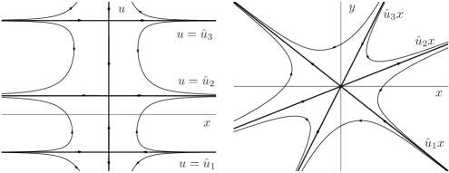
Figure 7: Correspondence between the phase plane $(x,u)$ of system (22) and neighborhood $\Omega$ of the origin of system (18). The case of six hyperbolic sectors

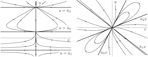
Figure 8: Correspondence between the phase plane $(x,u)$ of system (22) and neighborhood $\Omega$ of the origin of system (18). The case of two parabolic and two elliptic sectors

Thus we have that case (1) corresponds to 6 hyperbolic branches and 6 hyperbolic sectors (Fig. 7); cases (2)-(4) correspond to two hyperbolic and four parabolic branches or, respectively, two elliptic sectors and two parabolic sectors (Fig. 8), here four parabolic sectors described by Proposition 1 merge into two; cases (5)-(7) correspond to four hyperbolic and two parabolic branches, or to two hyperbolic and two parabolic sectors (Fig. 9).

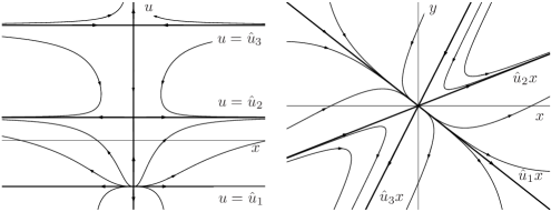
Figure 9: Correspondence between the phase plane $(x,u)$ of system (22) and neighborhood $\Omega$ of the origin of system (18). The case of two parabolic and two hyperbolic sectors

Now let $F_{1}(u)$ have only one real root. We can include the case $\hat{u}=0$ due to $(C1)$ and $(C2)$ ($F_{2}(v)$ has no real roots in this case). This root can correspond to a saddle or node equilibrium point $(0,\hat{u})$ of (22). The first case agrees (Proposition 1) with the presence of two hyperbolic sectors (Fig. 10); the second one agrees with the presence of two elliptic sectors (Fig. 11).

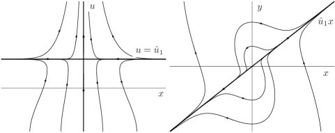
Figure 10: Correspondence between the phase plane $(x,u)$ of system (22) and neighborhood $\Omega$ of the origin of system (18). The case of two hyperbolic sectors

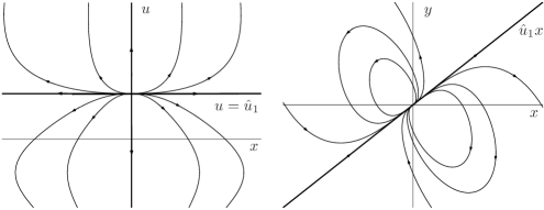
Figure 11: Correspondence between the phase plane $(x,u)$ of system (22) and neighborhood $\Omega$ of the origin of system (18). The case of two parabolic and two elliptic sectors

If polynomial $F_{1}(u)$ has two real roots which are not equal to zero, it follows from $(C1)$, $(C2)$ and Proposition 6 that $F_{2}(v)$ has three real roots and we should consider $F_{2}(v)$ instead of $F_{1}(u)$ (analogous to the case of three real roots of $F_{1}(u)$).

Polynomial $F_{1}(u)$ can have two real roots, and one of them $\hat{u}=0$. This necessarily implies (together with Proposition (6)) that $F_{2}(v)$ also has two real roots, one of them $\hat{v}=0$. So we have three roots ($\hat{u}\neq 0$ corresponds to $\hat{v}=1/\hat{u}$ which of the same type). Simple arguing shows that these three roots can be (1) three saddles (six hyperbolic sectors); (2) two nodes and a saddle (two elliptic and two parabolic sectors); (3) a node and two saddles (two parabolic and two hyperbolic sectors).

If $F_{1}(u)$ has no real root it implies that $F_{2}(v)$ has the only root $\hat{v}=0$ and this case is similar to the case of one real root of $F_{1}(u)$: two hyperbolic or two elliptic sectors depending on the type of $(0,\hat{v}=0)$.

Other cases are not possible in system (18) with $n=2$ that satisfies $(C1)$ and $(C2)$, which completes the proof. ∎

If we specify some additional conditions on (17), we can say more about asymptotics to the lines $y=0$ and $x=0$ of vector field (17). Namely, if

$$(C3)\qquad P_{n}(0,y)\equiv 0\Rightarrow P^{*}(0,y)\equiv 0,\quad Q_{n}(x,0)\equiv 0\Rightarrow Q^{*}(x,0)\equiv 0$$

hold, we can prove

Proposition 8.

Let $y=0$ consist of orbits of non-degenerate vector field (17) satisfying $(C3)$, and $\beta=q_{n,1}/{p_{n,1}}>1$. Then (17) has a family of $O$-orbits $y=c|x|^{\beta}(1+o(1))$, where $c$ is an arbitrary constant.

Proof.

If $y=0$ consists of orbits of vector field (17) then $\hat{u}=0$ is a root of $F_{1}(u)=-p_{0,n+1}u^{n+1}+\ldots+(q_{n,1}-p_{n,1})u+q_{n+1,0}$. It implies that $q_{n+1,0}=0$, and $y=0$ is a factor of $Q_{n}(x,y)$, from which $Q^{*}(x,0)\equiv 0$ follows (due to $(C3)$). From $(C1)$ it follows that $p_{n,1}\neq 0$. According to Proposition 3 the hyperbolic equilibrium point $(x=0,u=0)$ is a node because we assumed that $q_{n,1}/{p_{n,1}}>1$ which means $F_{1}^{\prime}(0)P_{n}(1,0)=p_{n,1}(q_{n,1}-p_{n,1})>0$. There is a family of characteristic orbits of the form $u=c|x|^{\beta-1}(1+o(1))$ where $c$ is an arbitrary constant. Returning to variables $x,\,y=ux$ completes the proof. ∎

Using the second blow-up transformation (20) we obtain

Proposition 9.

Let $x=0$ consist of orbits of non-degenerate vector field (17), and $\beta=p_{1,n}/{q_{1,n}}>1$. Then vector field (17) has a family of $O$-orbits $x=c|y|^{\beta}(1+o(1))$, where $c$ is an arbitrary constant.

The proof of Proposition 9 is similar to the proof of Proposition 8.

Proof of Theorem 3.

The proof follows from Theorem 7 and Propositions 8 and 9. ∎

General remarks.

Vector field (17) is a particular case of so-called vector field with a fixed Newton diagram (e.g., [45]). The conditions of existence of orbits with characteristic directions for vector fields with an arbitrary Newton diagram are also known [35, 36, 37]. The following facts are stated for a homogeneous case but can be carried onto more general situations almost literally.

Let

$$J_{n}=P_{n}(x,y)\frac{\partial}{\partial x}+Q_{n}(x,y)\frac{\partial}{\partial y}$$

be a homogeneous vector field having characteristic directions. The following theorem holds.

Theorem 8.

There exists a neighborhood $\Omega$ of singular point $O(0,0)$, such that vector field (17) is topologically equivalent to vector field $J_{n}$ in $\Omega$.

In case when $J_{n}$ has no orbits with characteristic directions point $O(0,0)$ is monodromic (this can be the case only if $n$ is odd). If we assume that

$$(C4)\quad\mbox{Polynomial $F(x,y)$ has no multiple complex factors}$$

holds, then the cases of focus or center can be identified.

Denote

$$l=\sum_{\textrm{Im}\,z>0}\textrm{res}_{z}\frac{P_{n}(1,u)}{F(1,u)}$$

the generalized first Lyapunov value.

Theorem 9.

Let $O(0,0)$ be a monodromic singular point of non-degenerate vector field $J_{n}$ satisfying $(C4)$. Then $O(0,0)$ is a focus if $l\neq 0$. This focus is attracting if $l<0$ and repelling if $l>0$.

Thus, in principle, it is possible to analyze non-hyperbolic equilibrium $O(0,0)$ of system (18) for an arbitrary $n$.

Acknowledgements.

The work of FSB has been supported in part by NSF Grant #634156 to Howard University.

References

- [1] Lotka AJ: Elements of physical biology. Baltimore: Williams & Wilkins Co; 1925.
- [2] Volterra V: Variazioni e fluttuazioni del numero d’individui in specie animali conviventi. Mem R Accad Naz dei Lincei Ser VI 1926, 2.
- [3] Kermack WO, McKendrick AG: A Contribution to the Mathematical Theory of Epidemics. Proceedings of the Royal Society of London Series A, Containing Papers of a Mathematical and Physical Character 1927, 115(772):700-721.
- [4] Holling CS: The components of predation as revealed by a study of small mammal predation of the European pine sawfly. Canadian Entomologist 1959, 91:293-320.
- [5] Holling, C.S.: Some characteristics of simple types of predation and parasitism. Canadian Entomologist 1959, 91:385-398.
- [6] Arditi R, Ginzburg LR: Coupling in Predator Prey Dynamics - Ratio-Dependence. Journal of Theoretical Biology 1989, 139(3):311-326.
- [7] Bazykin, A.D.: Nonlinear dynamics of interacting population, World Scientific (1998)
- [8] Hassell MP, Varley GC: New inductive population model for insect parasites and its bearing on biological control. Nature 1969, 223:1133-1136.
- [9] DeAngelis DL, Goldstein RA, O’Neill RV: A model for trophic interaction. Ecology 1975, 56:881-892.
- [10] Beddington JR: Mutual interference between parasites or predators and its effect on searching efficiency. Journal of Animal Ecology 1975, 51:331-340.
- [11] Abrams PA, Ginzburg LR: The nature of predation: prey dependent, ratio dependent or neither? Trends in Ecology & Evolution 2000, 15(8):337-341.
- [12] Akcakaya HR, Arditi R, Ginzburg LR: Ratio-Dependent Predation - an Abstraction That Works. Ecology 1995, 76(3):995-1004.
- [13] Berezovskaya F, Karev G, Arditi R: Parametric analysis of the ratio-dependent predator-prey model. Journal of Mathematical Biology 2001, 43(3):221-246.
- [14] Hsu SB, Hwang TW, Kuang Y: Global analysis of the Michaelis-Menten-type ratio-dependent predator-prey system. Journal of Mathematical Biology 2001, 42(6):489-506.
- [15] Jost C, Arino O, Arditi R: About deterministic extinction in ratio-dependent predator-prey models. Bulletin of Mathematical Biology 1999, 61(1):19-32.
- [16] Kuang Y, Beretta E: Global qualitative analysis of a ratio-dependent predator-prey system. Journal of Mathematical Biology 1998, 36(4):389-406.
- [17] Tang YL, Zhang WN: Heteroclinic bifurcation in a ratio-dependent predator-prey system. Journal of Mathematical Biology 2005, 50(6):699-712.
- [18] Xiao DM, Ruan SG: Global dynamics of a ratio-dependent predator-prey system. Journal of Mathematical Biology 2001, 43(3):268-290.
- [19] Diekmann O, Heesterbeek JAP: Mathematical Epidemiology of Infectious Diseases: Model Building, Analysis and Interpretation. New York: John Wiley; 2000.
- [20] McCallum H, Barlow N, Hone J: How should pathogen transmission be modelled? Trends in Ecology & Evolution 2001, 16(6):295-300.
- [21] May RM, Anderson RM: Transmission Dynamics of Hiv-Infection. Nature 1987, 326(6109):137-142.
- [22] Hethcote HW: The mathematics of infectious diseases. Siam Review 2000, 42(4):599-653.
- [23] Busenberg S, Cooke K: Vertically Transmitted Diseases. New York: Springer-Verlag; 1992.
- [24] Menalorca J, Hethcote HW: Dynamic-Models of Infectious-Diseases as Regulators of Population Sizes. Journal of Mathematical Biology 1992, 30(7):693-716.
- [25] Gao LQ, Hethcote HW: Disease Transmission Models with Density-Dependent Demographics. Journal of Mathematical Biology 1992, 30(7):717-731.
- [26] Busenberg S, Vargas C: Modeling Chagas’ desease: variable population size and demographic implications. In: Mathematical population dynamics. Edited by Arino O, Axelrod D, Kimmel M. New York: Marcel Dekker; 1991: 283-296.
- [27] Hwang TW, Kuang Y: Deterministic extinction effect of parasites on host populations. Journal of Mathematical Biology 2003, 46(1):17-30.
- [28] Berezovsky F, Karev G, Song B, Castillo-Chavez C: A simple epidemic model with surprising dynamics. Mathematical Biosciences and Engineering 2005, 2(1):133-152.
- [29] Hwang TW, Kuang Y: Host extinction dynamics in a simple parasite-host interaction model. Mathematical Biosciences and Engineering 2005, 2(4):743-751.
- [30] de Jong MCM, Diekmann O, Heesterbeek H: How does transmission of infection depend on population size? In: Epidemic Models: Their Structure and Relation to Data. Edited by Mollison D: Cambridge University Press; 1995: 84-94.
- [31] Novozhilov AS, Berezovskaya FS, Koonin EV, Karev GP: Mathematical modeling of tumor therapy with oncolytic viruses: Regimes with complete tumor elimination within the framework of deterministic models. Biology Direct 2006, 1(1):6.
- [32] de Pillis LG, Radunskaya AE, Wiseman CL: A Validated Mathematical Model of Cell-Mediated Immune Response to Tumor Growth. Cancer Research 65, 7950-7958 (2005)
- [33] Andronov A.A., Leontovich E.A., Gordon, I.I., Maier A.G. (1973) Qualitative Theory of second-order dynamic systems. John Wiley & Sons. Translation
- [34] Berezovskaya F.S. (1976) About asymptotics of trajectories of a system of two differential equations. Dep. in the All-Union Information Center (USSR), No 3447-76, 17 p.(in Russian)
- [35] Berezovskaya F.S. (1978) Topological normal form for a system of two differential equations. Russian Math. Surveys, 33:2, 227-228.
- [36] Berezovskaya F.S. (1995) The main topological part of plane vector fields with fixed Newton diagram. In: Proceedings on Singularity Theory, D.T. Le, K. Saito, B. Teissier (eds), 55-73, Word Scientific: Singapore, New Jersey, London, Hong Kong.
- [37] Berezovskaya F.S., Medvedeva N.B. (1994) A complicated singular point of ”center-focus” type and the Newton diagram. Selecta Mathematica formely Sovietica, v.13, 1
- [38] Bruno A.D. Power geometry in algebraic and differential equations. IMPRINT. Amsterdam, New York: Elsevier, 2000
- [39] Dumortier F.(1977) Singularities of vector fields in the plane. J. Differential equations, 23, 53-106.
- [40] Parato KA, Senger D, Forsyth PA, Bell JC: Recent progress in the battle between oncolytic viruses and tumours. Nat Rev Cancer 2005, 5(12):965-976.
- [41] Wodarz D: Viruses as antitumor weapons: defining conditions for tumor remission. Cancer Res 2001, 61(8):3501-3507.
- [42] Harrison D, Sauthoff H, Heitner S, Jagirdar J, Rom WN, Hay JG: Wild-type adenovirus decreases tumor xenograft growth, but despite viral persistence complete tumor responses are rarely achieved–deletion of the viral E1b-19-kD gene increases the viral oncolytic effect. Hum Gene Ther 2001, 12(10):1323-1332.
- [43] Hsu SB, Hwang TW, Kuang Y: Rich dynamics of a ratio-dependent one-prey two-predators model. Journal of Mathematical Biology 2001, 43(5):377-396.
- [44] Hsu SB, Hwang TW, Kuang Y: A ratio-dependent food chain model and its applications to biological control. Mathematical Biosciences 2003, 181(1):55-83.
- [45] Arnold VI, Ilyashenko YuS: Ordinary differential equations, 1. Encyclopedia of mathematical science, Vol. 1, Springer, 1994.