Percolation on fitness landscapes: effects of correlation, phenotype, and incompatibilities

Abstract We study how correlations in the random fitness assignment may affect the structure of fitness landscapes. We consider three classes of fitness models. The first is a continuous phenotype space in which individuals are characterized by a large number of continuously varying traits such as size, weight, color, or concentrations of gene products which directly affect fitness. The second is a simple model that explicitly describes genotype-to-phenotype and phenotype-to-fitness maps allowing for neutrality at both phenotype and fitness levels and resulting in a fitness landscape with tunable correlation length. The third is a class of models in which particular combinations of alleles or values of phenotypic characters are “incompatible” in the sense that the resulting genotypes or phenotypes have reduced (or zero) fitness. This class of models can be viewed as a generalization of the canonical Bateson-Dobzhansky-Muller model of speciation. We also demonstrate that the discrete $NK$ model shares some signature properties of models with high correlations. Throughout the paper, our focus is on the percolation threshold, on the number, size and structure of connected clusters, and on the number of viable genotypes.

Key words: fitness landscapes, percolation, nearly neutral networks, genetic incompatibilities

1 Introduction

The notion of fitness landscapes, introduced by a theoretical evolutionary biologist Sewall Wright in 1932 (see also Kauffman, 1993; Gavrilets, 2004), has proved extremely useful both in biology and well outside of it. In the standard interpretation, a fitness landscape is a relationship between a set of genes (or a set of quantitative characters) and a measure of fitness (e.g. viability, fertility, or mating success). In Wright’s original formulation the set of genes (or quantitative characters) is the property of an individual. However, the notion of fitness landscapes can be generalized to the level of a mating pair, or even a population of individuals (Gavrilets,, 2004).

To date, most empirical information on fitness landscapes in biological applications has come from studies of RNA (e.g., Schuster, 1995; Huynen et al., 1996; Fontana and Schuster, 1998), proteins (e.g., Lipman and Wilbur, 1991; Martinez et al., 1996; Rost, 1997), viruses (e.g., Burch and Chao, 1999, 2004), bacteria (e.g., Elena and Lenski, 2003; Woods et al., 2006), and artificial life (e.g., Lenski et al., 1999; Wilke et al., 2001). The three paradigmatic landscapes — rugged, single-peak, and flat — emphasizing particular features of fitness landscapes have been the focus of most of the earlier theoretical work (reviewed in Kauffman, 1993; Gavrilets, 2004). These landscapes have found numerous applications with regards to the dynamics of adaptation (e.g., Kauffman and Levin, 1987; Kauffman, 1993; Orr, 2006b ; Orr, 2006a ) and neutral molecular evolution (e.g., Derrida and Peliti, 1991).

More recently, it was realized that the dimensionality of most biologically interesting fitness landscapes is enormous and that this huge dimensionality brings some new properties which one does not observe in low-dimensional landscapes (e.g. in two- or three-dimensional geographic landscapes). In particular, multidimensional landscapes are generically characterized by the existence of neutral and nearly neutral networks (also referred to as holey fitness landscapes) that extend throughout the landscapes and that can dramatically affect the evolutionary dynamics of the populations (Gavrilets,, 1997; Gavrilets and Gravner,, 1997; Reidys et al.,, 1997; Gavrilets,, 2004; Reidys et al.,, 2001; Reidys and Stadler,, 2001, 2002).

An important property of fitness landscapes is their correlation pattern. A common measure for the strength of dependence is the correlation function $\rho$ measuring the correlation of fitnesses of pairs of individual at a distance (e.g., Hamming) $d$ from each other in the genotype (or phenotype) space:

$$\rho(d)=\frac{\operatorname{cov}[w(.),w(.)]_{d}}{\operatorname{var}(w)}$$ (1)

(Eigen et al.,, 1989). Here, the term in the numerator is the covariance of fitnesses of two individuals conditioned on them being at distance $d$, and $\operatorname{var}(w)$ is the variance in fitness over the whole fitness landscape. For uncorrelated landscapes, $\rho(d)=0$ for $d>0$. In contrast, for highly correlated landscapes, $\rho(d)$ decreases with $d$ very slowly.

The aim of this paper is to extend our previous work (Gavrilets and Gravner,, 1997) in a number of directions paying special attention to the question of how correlations in the random fitness assignment may affect the structure of genotype and phenotype spaces. For the resulting random fitness landscapes, we shed some light on issues such as the number of viable genotypes, number of connected clusters of viable genotypes and their size distribution, existence thresholds, and number of possible fitnesses.

To this end, we introduce a variety of models, which could be divided into two essentially different classes: those with local correlations, and those with global correlations. As we will see, techniques used to analyze these models, and answers we obtain, differ significantly. We use a mixture of analytical and computational techniques; it is perhaps necessary to point out that these models are very far from trivial, and one is quickly led to outstanding open problems in probability theory and computer science.

We start (in Section 2) by briefly reviewing some results from Gavrilets and Gravner, (1997). In Section 3 we generalize these results for the case of a continuous phenotype space when individuals are characterized by a large number of continuously varying traits such as size, weight, color, or the concentrations of some gene products. The latter interpretation of the phenotype space may be particularly relevant given the rise of proteomics and the growing interest in gene regulatory networks.

The main idea behind our local correlations model studies in Section 4 is fitness assignment conformity. Namely, one randomly divides the genotype space into components which are forced to have the same phenotype; then, each different phenotype is independently assigned a random fitness. This leads to a simple two-parameter model, in which one parameter determines the density of viable genotypes, and the other the correlations between them. We argue that the probability of existence of a giant cluster (which swallows a positive proportion of all viable genotypes) is a non-monotone function of the correlation parameter and identify the critical surface at which this probability jumps almost from 0 to 1. In Section 4 we also investigate the effects of interaction between conformity structure and fitness assignment.

Section 5 introduces our basic global correlation model, one in which genotypes are eliminated due to random pairwise incompatibilities between alleles. This is equivalent to a random version of SAT problem, which is the canonical constraint satisfaction problem in computer science. In general, a SAT problem involves a set of Boolean variables and their negations that are strung together with OR symbols into clauses. The clauses are joined by AND symbols into a formula. A SAT problem asks one to decide, whether the variables can be assigned values that will make the formula true. An important special case, $K$-SAT, has the length of each clause fixed at $K$. Arguably, SAT is the most important class of problems in complexity theory. In fact, the general SAT was the first known NP-complete problem and was established as such by S. Cook in 1971 (Cook, 1971). Even considerable simplifications, such as the $3$-SAT (see Section 5.4), remain NP-complete, although $2$-SAT (see Section 5.1) can be solved efficiently by a simple algorithm. See e.g. Korte and Vygen, (2005) for a comprehensive presentation of the theory. Difficulties in analyzing random SAT problems, in which formulas are chosen at random, in many ways mirror their complexity classes, but even random $2$-SAT presents significant challenges (de la Vega,, 2001; Bollobás et al.,, 1994). In our present interpretation, the main reason for these difficulties is that correlations are so high that the expected number of viable genotypes may be exponentially large, while at the same time the probability that even one viable genotype exists is very low. In Section 5, we further illuminate this issue by showing that connected viable clusters must contain fairly large sub-cubes, and that the number of such clusters is, in a proper interpretation, finite. The relevance to both types of models for discrete and continuous phenotype spaces is also discussed, with particular emphasis on the existence of viable phenotypes in the presence of incompatibilities. Section 5 also contains a brief review of the existing theory on higher order incompatibilities.

In Section 6 we demonstrate how the discrete $NK$ model shares some signature properties of models with high correlations. In Section 7 we summarize our results and discuss their biological relevance. The proofs of our major results are relegated to Appendices A–E.

2 The basic case: binary hypercube and independent binary fitness

We begin with a brief review of the basic setup, from Gavrilets and Gravner, (1997) and Gavrilets, (2004). The binary hypercube consists of all $n$–long arrays of bits, or alleles, that is ${\mathcal{G}}=\{0,1\}^{n}$. This is our genotype space. Genotypes are linked by edges induced by bit-flips, i.e., mutations at a single locus, for example, for $n=4$, a sequence of mutations might look like

$$0000\leftrightarrow 1000\leftrightarrow 1001\leftrightarrow 1101\leftrightarrow 1100.$$

The (Hamming) distance $d(x,y)$ between $x\in{\mathcal{G}}$ and $y\in{\mathcal{G}}$ is the number of coordinates in which $x$ and $y$ differ or, equivalently, the least number of mutations which connect $x$ and $y$.

The fitness of each genotype $x$ is denoted by $w(x)$. We will describe several ways to prescribe the fitness $w$ at random, according to some probability measure $P$ on the $2^{2^{n}}$ possible assignments. Then we say that an event $A_{n}$ happens asymptotically almost surely (a. a. s.) if $P(A_{n})\to 1$ as $n\to\infty$. Typically, $A_{n}$ will capture some important property of (random) clusters of genotypes.

We commonly assume that $w(x)\in\{0,1\}$ so that $x$ is either viable ($w(x)=1$) or inviable ($w(x)=0$). As a natural starting point, Gavrilets and Gravner, (1997) considered uncorrelated landscapes, in which $w(x)$ is chosen to be 1 with probability $p_{v}$, for each $x$ independently of others. We assume this setup for the rest of this section and note that this is a well-studied problem in mathematical literature, although it presents considerable technical difficulties and some issues are still not completely resolved.

Given a particular fitness assignment, viable genotypes form a subset of ${\mathcal{G}}$, which is divided into connected components or clusters. For example, with $n=4$, if $0000$ is viable, but its 4 neighbors $1000$, $0100$, $0010$, and $0001$ are not, then it is isolated in its own cluster.

Perhaps the most basic result determines the connectivity threshold (Toman,, 1979): when $p_{v}>1/2$, the set of all viable genotypes is connected a. a. s. By contrast, when $p_{v}<1/2$, the set of viable genotypes is not connected a. a. s. This is easily understood, as the connectedness is closely linked to isolated genotypes, whose expected number is $2^{n}p_{v}(1-p_{v})^{n}$. This expectation makes a transition from exponentially large to exponentially small at $p_{v}=1/2$. The events $\{x$ is isolated$\}$, $x\in{\mathcal{G}}$, are only weakly correlated, which implies that when $p_{v}<1/2$ there are exponentially many isolated genotypes with high probability, while when $p_{v}>1/2$, a separate argument shows that the event that the set of viable genotypes contains no isolated vertex but is not connected becomes very unlikely for large $n$. This is perhaps the clearest instance of the local method: a local property (no isolated genotypes) is a. a. s. equivalent to a global one (connectivity).

Connectivity is clearly too much to ask for, as $p_{v}$ above $1/2$ is not biologically realistic. Instead, one should look for a weaker property which has a chance of occurring at small $p_{v}$. Such a property is percolation, a. k. a. existence of the giant component. For this, we scale $p_{v}=\lambda_{v}/n$, for a constant $\lambda_{v}$. When $\lambda_{v}>1$, the set of viable genotypes percolates, that is, it a. a. s. contains a component of at least $c\cdot n^{-1}2^{n}$ genotypes, with all other components of at most polynomial (in $n$) size. When $\lambda_{v}<1$, the largest component is a. a. s. of size $Cn$. Here and below, $c$ and $C$ are some constants. These are results from Bollobás et al., (1994).

The local method that correctly identifies the percolation threshold is a little more sophisticated than the one for the connectivity threshold, and uses branching processes with Poisson offspring distribution — hence we introduce notation Poisson($\lambda$) for a Poisson distribution with mean $\lambda$. Viewed from, say, genotype $0\dots 0$, the binary hypercube locally approximates a tree with uniform degree $n$. Thus viable genotypes approximate a branching process in which every node has the number of successors distributed binomially with parameters $n-1$ and $p$, hence this random number has mean about $\lambda_{v}$ and is approximately Poisson($\lambda_{v}$). When $\lambda_{v}>1$, such a branching process survives forever with probability $1-\delta>0$, where $\delta=\delta(\lambda_{v})$, and $\delta(\lambda)$ is given by the implicit equation

$$\delta=e^{\lambda(\delta-1)}.$$ (2)

(e.g., Athreya and Ney, 1971). Large trees of viable genotypes created by the branching processes which emanate from viable genotypes merge into a very large (“giant”) connected set. On the other hand, when $\lambda_{v}<1$ the branching process dies out with probability 1.

The condition $\lambda_{v}>1$ for the existence of the giant component can be loosely rewritten as

$$p_{v}>\frac{1}{n}.$$ (3)

This shows that the larger the dimensionality $n$ of the genotype space, the smaller values of the probability of being viable $p_{v}$ will result in the existence of the giant component. See Gavrilets and Gravner, (1997); Gavrilets, (1997, 2004); Skipper, (2004); Pigliucci, (2006) for discussions of biological significance and implications of this important result.

3 Percolation in a continuous phenotype space

In this section we will assume that individuals are characterized by $n$ continuous traits (such as size, weight, color, or concentrations of particular gene products). To be precise, we let ${\mathcal{P}}=[0,1]^{n}$ be the phenotype space.

We begin with the extension of the notion of independent viability. The most straightforward analogue of the discrete genotype space considered in the previous section involves Poisson point location in $\cal{P}$, obtained by generating a Poisson($\lambda$) random variable $N$, and then choosing points $x_{1},\dots,x_{N}\in{\mathcal{P}}$ uniformly at random. These will be interpreted as peaks of equal height in the fitness landscape. Another parameter is a small $r>0$, which can be interpreted as measuring how harsh the environment is: any phenotype within $r$ of one of the peaks is declared viable and any phenotype not within $r$ of one of the peaks is declared inviable. For simplicity, we will assume “within $r$” to mean that “every coordinate differs by at most $r$,” i.e., distance is measured in the ($n$-dimensional) $\ell^{\infty}$ norm $||\cdot||_{\infty}$. Note that this makes the set of viable genotypes correlated, albeit the range of correlations is limited to $2r$.

Our most basic question is whether a positive proportion of viable phenotypes is connected together into a giant cluster. Note that the probability $p_{v}$ that a random point in ${\mathcal{P}}$ is viable is equal to the probability that there is a “peak” within $r$ from this point. Therefore,

$$p_{v}=1-\exp\left[-\lambda(2r)^{n}\right]\approx\lambda(2r)^{n}.$$

This is also the expected combined volume of viable phenotypes.

We will consider peaks $x_{i}$ and $x_{j}$ to be neighbors if they share a viable phenotype, that is, if their $r$-neighborhoods overlap, or equivalently, if $||x_{i}-x_{j}||_{\infty}<2r$. Two viable phenotypes $y_{1}$ and $y_{2}$ are connected if they are, respectively, within $r$ of peaks $x_{1}$ and $x_{2}$, and $x_{1}$ and $x_{2}$ are connected to each other via a chain of neighboring peaks.

By the standard branching process comparison, the necessary condition for the existence of a giant cluster is that a “peak” $x$ is connected to more than one other “peak” on the average. All peaks within $2r$ of the focal peak are connected to the latter. Therefore, if $\mu$ is the expected number of peaks connected to $x$, then

$$\mu=\lambda\cdot(4r)^{n},$$

and $\mu>1$ is necessary for percolation. As demonstrated by Penrose, (1996) (for a different choice of the norm, but the proof is the same), this condition becomes sufficient when $n$ is large. Note that the expected number $\lambda$ of peaks can be written as $\mu\cdot(4r)^{-n}$.

If $\mu>1$ and fixed, then a. a. s. a positive proportion of all peaks (that is, $cN$ peaks, where $c=c(\mu)>0$) are connected in one “giant” component, while the remaining connected components are all of size ${\mathcal{O}}(\log N)$. On the other hand, if $\mu<1$, all components are a. a. s. of size ${\mathcal{O}}(\log N)$.

The condition $\mu>1$ for the existence of the giant component of viable phenotypes can be loosely rewritten as

$$p_{v}>\frac{1}{2^{n}}.$$ (4)

This shows that viable phenotypes are likely to form a large connected cluster even when one is very unlikely to hit one of them at random, if $n$ is even moderately large. The same conclusion and the same threshold are valid if instead of $n$-cubes we use $n$-spheres of a constant radius.

The percolation threshold in the continuous phenotype space given by inequality (4) is much smaller than that in the discrete genotype space which is given by inequality (3). An intuitive reason for this is that continuous space offers a viable point a much greater opportunity to be connected to a large cluster. Indeed, in the discrete genotype space there are $n$ neighbors per each genotype. In contrast, in the continuous phenotype space, the ratio of the volume of the space where neigboring peaks can be located (which has radius $2r$) to the volume of the focal $n$-cube (which has radius $r$) is $2^{n}$.

4 Percolation in a correlated landscape with phenotypic neutrality

The standard paradigm in biology is that the relationship between genotype and fitness is mediated by phenotype (i.e., observable characteristics of individuals). Both the genotype-to-phenotype and phenotype-to-fitness maps are typically not one-to-one. Here, we formulate a simple model capturing these properties which also results in a correlated fitness landscape. Below we will call mutations that do not change phenotype conformist. These mutations represent a subset of neutral mutations that do not change fitness.

We propose the following two-step model. To begin the first step, we make each pair of genotypes $x$ and $y$ in a binary hypercube ${\mathcal{G}}$ independently conformist with probability $p_{d(x,y)}$ where $d(x,y)$ is the Hamming distance between $x$ and $y$. We then declare $x$ and $y$ to belong to the same conformist cluster if they are linked by a chain of conformist pairs. This version of long-range percolation model (cf., Berger, 2004; Biskup, 2004) divides the set of genotypes ${\mathcal{G}}$ into conformist clusters. We postulate that all genotypes in the same conformist cluster have the same phenotype. Therefore, genetic changes represented by a change from one member of a conformist cluster to another (i.e., single or multiple mutations) are phenotypically neutral.

In the second step, we make each conformist cluster independently viable with probability $p_{v}=\lambda_{v}/n$. This generates a random set of viable genotypes, and we aim to investigate when this set has a large connected component.

For example, the “genotype” can be a linear RNA sequence. This sequence folds into a 2-dimensional molecule which has a particular structure (or “shape”), and corresponds to our “phenotype.” Finally, the molecule itself has a particular function, e.g., to bind to a specific part of the cell or to another molecule. A measure of how well this can be accomplished is represented by our “fitness.”

The distribution of conformist clusters depends on the probabilities $p_{1},p_{2},p_{3},\dots$ which determine how the conformity probability varies with distance. Here we will study the case when $p_{1}=p_{e}>0,p_{2}=p_{3}=...=0$ (Häggström,, 2001). It is then very convenient for the mathematical analysis that a pair $x$ and $y$ can be conformist only when they are linked by an edge — therefore we can talk about conformist edges or equivalently conformist mutations. (Note however that it is possible that nearest neighbors $x$ and $y$ are in the same conformist cluster even if the edge between them is non-conformist.)

Figure 1 illustrates our 2-step procedure on a four-dimensional example.

We expect that a more general model with $p_{i}$ declining fast enough with $i$ is just a smeared version of this basic one, and its properties are not likely to differ from those of the simpler model. We conjecture that for our purposes, “fast enough” decrease should be exponential with a rate logarithmically increasing in the dimension $n$, e.g. for large $k$,

$$p_{k}\leq\exp(-\alpha(\log n)k),$$

for some $\alpha>1$. (This is expected to be so because in this case the expected number of neighbors of the focal genotype is finite.)

We observe that the first step of our procedure is an edge version of the percolation model discussed in the second section, with a similar giant component transition (Bollobás et al.,, 1992). Namely, let $p_{1}=p_{e}=\lambda_{e}/n$. Then, if $\lambda_{e}>1$, there is a. a. s. one giant conformist cluster of size $c\cdot 2^{n}$, with all others of size at most $Cn$. In contrast, if $\lambda_{e}<1$ all conformist clusters are of size at most $Cn$. Note that the number of conformist clusters is always on the order $2^{n}$. In fact, even the number of “non-conformist” (i.e., isolated) clusters is a. a. s. asymptotic to $e^{-\lambda_{e}}2^{n}$, as $P(x\ \text{is isolated})=(1-\lambda_{e}/n)^{n}$.

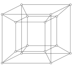
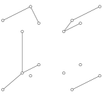
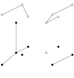
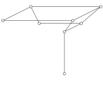
Figure 1: A four-dimensional example: start with the cube ${\mathcal{G}}^{4}$ (top left), create conformist clusters by randomly eliminating each edge with probability $1-p_{e}$ (top right), remove each conformist cluster with probability $1-p_{v}$ (bottom left, removed vertices are black) and finally consider connected components of the remaining vertices (bottom right, there is just one component in this case).

Denote by $x\leftrightsquigarrow y$ (resp. $x{\,\,\leftrightsquigarrow\!\!\!\!\!\!\!\!/\;\,\,\,}y$) the event that $x$ and $y$ are (resp. are not) in the same conformist cluster. First, we note that the probability $P(x\leftrightsquigarrow y)$ that two genotypes belong to the same conformist cluster depends on the Hamming distance $d(x,y)$ between them, and on $p_{e}=\lambda_{e}/n$. In particular, we show in Appendix A that, if $\lambda_{e}<1$ and $d(x,y)=k$ is fixed, then

$$k!p_{e}^{k}(1-O(n^{-2}))\leq P(x\leftrightsquigarrow y)\leq k!p_{e}^{k}(1+O(n^{-1}\log{n})).$$ (5)

The dominant contribution $k!p_{e}^{k}$ is simply the expected number of conformist pathways between $x$ and $y$ that are of shortest possible length.

It is also important to note that, for every $x\in{\mathcal{G}}$, the probability $P(x$ is viable$)=p_{v}$, therefore it does not depend on $p_{e}$. Moreover, for $x,y\in{\mathcal{G}}$,

$$P(x\text{ and }y\text{ viable})-p_{v}^{2}$$

$$=P(x\text{ and }y\text{ viable},x\leftrightsquigarrow y)+P(x\text{ and }y\text{ viable},x{\,\,\leftrightsquigarrow\!\!\!\!\!\!\!\!/\;\,\,\,}y)-p_{v}^{2}$$

$$=p_{v}P(x\leftrightsquigarrow y)+p_{v}^{2}\cdot P(x{\,\,\leftrightsquigarrow\!\!\!\!\!\!\!\!/\;\,\,\,}y)-p_{v}^{2}$$

$$=p_{v}(1-p_{v})P(x\leftrightsquigarrow y)\geq 0.$$

Therefore, the correlation function (1) is

$$\rho(x,y)=P(x\leftrightsquigarrow y),$$ (6)

which clearly increases with $p_{e}$ and, thus, with $\lambda_{e}$. Therefore, this model has tunable positive correlations controlled by the parameter $\lambda_{e}$, whose value does not affect the expected number of viable genotypes. The correlation function $\rho(x,y)$ decreases exponentially with distance $d(x,y)$ when $\lambda_{e}<1$, and is bounded below when $\lambda_{e}>1$. Nevertheless, as we will see below, we can effectively use local methods for all values of $\lambda_{e}$.

4.1 Threshold surface for percolation

Proceeding by the local branching process heuristics, we reason that a surviving node on the branching tree can have two types of descendants: those that are connected by conformist mutations and those that are in different conformist clusters and thus independently viable. Therefore the number of descendants is approximately Poisson($\lambda_{e}+\lambda_{v}$). This can only work when $\lambda_{e}<1$, as otherwise the correlations are global.

If $\lambda_{e}>1$, we need to eliminate the entire conformist giant component, which is a. a. s. inviable. Locally, we condition on the (supercritical) branching process of the supposed descendant to die out. Such conditioned process is a subcritical branching process, with Poisson $(\lambda_{e}\delta)$ distribution of successors (Athreya and Ney,, 1971) where $\delta=\delta(\lambda_{e})$ is given by the equation (2). This gives the conformist contribution, to which we add the independent Poisson$(\lambda_{v}\delta)$ contribution.

Figure 2: Simulated $\lambda_{v}^{m}$ (long dashes) and $\lambda_{v}^{M}$ (short dashes), and $\zeta$ (solid) plotted against $\lambda_{e}$, for $n=10,\dots,20$, and models from Section 4.1 (left frame) and Section 4.2 (right frame). Lower bounds increase with $n$, and upper bounds decrease, for this range of $n$.

To have a convenient summary of the conclusions above, assume that $\lambda_{e}$ is fixed and let $\zeta(\lambda_{e})$ be the smallest $\lambda_{v}$ which a. a. s. ensures the giant component, i.e.,

$$\zeta(\lambda_{e})=\inf\{\lambda_{v}:\text{a cluster of at least }cn^{-1}2^{n}\text{ viable genotypes exists a.~{}a.~{}s.~{}for some }c>0\}.$$

One would expect that for $\lambda_{v}<\zeta(\lambda_{e})$ all components are a. a. s. of size at most $Cn$. The asymptotic critical curve is given by $\lambda_{v}=\zeta(\lambda_{e})$, where

$$\zeta(\lambda)=\begin{cases}1-\lambda&\qquad\text{if }\lambda\in[0,1],\\ \frac{1}{\delta}-\lambda&\qquad\text{if }\lambda\in[1,\infty).\end{cases}$$ (7)

Having only a heuristic proof of this, we resort to computer simulations for confirmation. For this, we indicate global connectivity with the event $A$ that a genotype within distance 2 of $0\dots 0$ is connected (through viable genotypes) to a genotype within distance 2 of $1\dots 1$. We make this choice because the distance 2 is the smallest that works with asymptotic certainty. Indeed, the genotypes $0\dots 0$ and $1\dots 1$ are likely to be inviable. Even the number of viable genotypes within distance one of each of these is only of constant order, so even in the percolation regime the probability of connectivity between a viable genotype within distance one of $0\dots 0$ and a viable one within distance one of $1\dots 1$ does not converge to 1 but is of a nontrivial constant order. By contrast, there are about $n^{2}$ vertices within distance 2 of $0\dots 0$ among which of order $n$ are viable.

When $\lambda_{v}>\zeta(\lambda_{e})$ the probability of the event $A$ should therefore be (exponentially) close to 1. On the other hand, when $\lambda_{v}<\zeta(\lambda_{e})$ the probability that a connected component within distance 2 of either $0\dots 0$ or $1\dots 1$ extends for distance of the order $n$ is exponentially small. We further define the critical curves

$$\lambda_{v}^{m}=\; \lambda_{v} P(A)>0.1$$the smallest for which ,

$$\lambda_{v}^{M}=\; \lambda_{v} P(A)<0.9$$the largest for which .

We approximated $\lambda_{v}^{m}$ and $\lambda_{v}^{M}$ for $n=10,\dots,20$ and $\lambda_{e}=0(0.1)2$, with 1000 independent realizations of each choice of $n$, $\lambda_{e}$, and $\lambda_{v}$. We used the linear cluster algorithm described in Sedgewick, (1997). The results are depicted in Figure 1. Unfortunately, simulations above $n\approx 20$ are not feasible.

From Figure 2 we observe that:

• Even for low $n$, both critical curves approximate well the overall shape of the theoretical limit curve $\zeta$.

• $\lambda_{v}^{m}$ and $\lambda_{v}^{M}$ get closer faster than they converge to $\zeta$. Consequently, one can expect that $P(A)$ makes a very sharp jump from near 0 to near 1 even for moderate $n$.

• For $\lambda_{e}<1$, $\lambda_{v}^{m}$ tends to be above the limit curve. This is not really surprising, as the local argument always gives an upper bound on the probability $P(A)$ of event $A$. Further, the approximation of $\lambda_{v}^{m}$ deteriorates near $\lambda_{e}=2$, which stems from the possibility of survival of the giant component in this regime.

What is clear from the heuristics and simulations is that conformist mutations, and thus correlations, significantly affect the probability of long range connectivity in the genotype space. The effect is not monotone: the most advantageous choice is when the correlations are at the point of phase transition between between local and global.

To intuitively understand why percolation occurs the easiest with $\lambda_{e}\approx 1$, it helps to think of the model as a branching process on clusters rather than on genotypes. For a genotype on a viable cluster, there is a number of neighboring clusters and each of these is viable with probability $p_{v}$. If $\lambda_{e}<1$, then the probability that any two of the neighboring genotypes are in the same cluster is $o(1)$, so there are asymptotically exactly $n$ clusters neighboring the present cluster. Consequently, the overall number of descendants will be greater if the size of these clusters is greater on average; which is exactly what happens as $\lambda_{e}$ increases towards 1. If $\lambda_{e}>1$, then there is a positive proportion of the neighboring genotypes that are in the giant cluster. This giant cluster is likely to be inviable, so the parameter $\lambda_{v}$ must be greater to compensate for its loss.

4.2 Correlations between conformity and viability

In the previous model, the viability probability $p_{v}$ was independent of the conformity structure. Mainly to investigate the robustness of our conclusions, we consider a simple generalization in which there are either positive or negative correlations between conformity and fitness. While more sophisticated models are possible, the one below is chosen for its amenability to relatively simple analysis.

Assume now that conformist clusters are formed as before (i.e., with edges being conformist with probability $p_{e}=\lambda_{e}/n$), are still independently viable, but now the probability of their viability depends on their size. We will consider the simple case when an isolated genotype (one might call it non-conformist) is viable with probability $p_{0}=\lambda_{0}/n$, while a conformist cluster of size larger than 1 is viable with probability $p_{1}=\lambda_{1}/n$.

In this case

$$P(x\text{ is viable})=(1-p_{e})^{n}p_{0}+(1-(1-p_{e})^{n})p_{1}\sim\frac{1}{n}\left(e^{-\lambda_{e}}\lambda_{0}+(1-e^{-\lambda_{e}})\lambda_{1}\right).$$

Moreover, by a similar calculation as before,

$$P(x\text{ and }y\text{ viable})-P(x\text{ viable})^{2}$$

$$=p_{1}(1-p_{1})P(x\leftrightsquigarrow y)+P(x\text{ non-conformist})^{2}p_{e}(p_{0}-p_{1})^{2}\cdot 1_{\{d(x,y)=1\}}.$$

Here, the last factor is the indicator of the set $\{(x,y),d(x,y)=1\}$, which equals $1$ if $d(x,y)=1$ and $0$ otherwise. Therefore, for $d(x,y)\geq 2$, the correlation function (1) is

$$\rho(x,y)\sim\frac{\lambda_{1}}{e^{-\lambda_{e}}\lambda_{0}+(1-e^{-\lambda_{e}})\lambda_{1}}P(x\leftrightsquigarrow y),$$

which is smaller than before iff $\lambda_{1}<\lambda_{0}$. However, it has the same asymptotic properties unless $\lambda_{1}=0$.

Assume first that $\lambda_{e}<1$. The local analysis now leads to a multi-type branching process (Athreya and Ney,, 1971) with three types: NC (non-conformist node), CI (non-isolated node independently viable, so no conformist edge is accounted for), and CC (non-isolated node viable by conformity, so a conformist edge is accounted for).

Note first that a genotype is non-conformist with probability about $e^{-\lambda_{e}}$. Hence a node of any of the three types creates a Poisson($e^{-\lambda_{e}}\lambda_{1}$) number of type NC descendants, and a Poisson($(1-e^{-\lambda_{e}})\lambda_{1}$) number of type CI descendants. In addition, the type CI creates a Poisson($\lambda_{e}$), conditioned on being nonzero, number of descendants of type CC and type CC creates a Poisson($\lambda_{e}$) number of descendants of type CC. Thus the matrix of expectations, in which the $ij$th entry is the expectation of the number of type $j$ descendants from type $i$, is

$$M=\begin{bmatrix}e^{-\lambda_{e}}\lambda_{0}&\left(1-e^{-\lambda_{e}}\right)\lambda_{1}&0\\ e^{-\lambda_{e}}\lambda_{0}&\left(1-e^{-\lambda_{e}}\right)\lambda_{1}&\lambda_{e}/(1-e^{-\lambda_{e}})\\ e^{-\lambda_{e}}\lambda_{0}&\left(1-e^{-\lambda_{e}}\right)\lambda_{1}&\lambda_{e}\end{bmatrix}\quad.$$

When $\lambda_{e}>1$, $\lambda_{e}$ needs to be replaced by $\lambda_{e}\delta$, and $\lambda_{1}$ by $\lambda_{1}\delta$, where $\delta=\delta(\lambda_{e})$ is given by  (2).

It follows from the theory of multi-type branching processes (Athreya and Ney,, 1971) that the critical surface for survival of a multi-type branching process is given by $\det(M-1)=0$.

The simplest case is when only non-conformist genotypes may be viable, i.e., $\lambda_{1}=0$. In this case the critical surface is given by $\lambda_{0}e^{-\lambda_{e}}=1$ (Pitman, unpub.). Not surprisingly, the critical $\lambda_{0}$ to achieve global connectivity strictly increases with $\lambda_{e}$, which is the result of negative correlations between conformity and viability.

The other extreme is when non-conformist genotypes are inviable, i.e., $\lambda_{0}=0$. As an easy computation demonstrates, the critical curve is now given by $\lambda_{1}=\zeta(\lambda_{e})$, where

$$\zeta(\lambda)=\begin{cases}\frac{1-\lambda}{\lambda e^{-\lambda}+1-e^{-\lambda}}&\qquad\text{if }\lambda\in\{0,1\},\\ \frac{\rho^{-1}-\lambda}{\lambda e^{-\lambda}+1-e^{-\lambda\rho}}&\qquad\text{if }\lambda\in[1,\infty).\end{cases}$$ (8)

Note that $\zeta(\lambda)\to\infty$ as $\lambda\to 0$. We carried out exactly the same simulations as before. These are also featured in Figure 2 (right frame), and again confirm our local heuristics. We conclude that positive correlations between viability and conformity tend to lead to a V-shaped critical curve, whose sharpness at critical conformity $\lambda_{e}=1$ increases with the size of correlations. In short, then, correlations help more if viability probability increases with size of conformist clusters.

5 Percolation in incompatibility models

In the model considered in the previous section correlations rapidly decreased with distance. This property made local analysis possible. The models we introduce now are fundamentally different in the sense that correlations are so high that the local method gives a wrong answer.

In the previous sections, in constructing fitness landscapes we were assigning fitness to individual genotypes or phenotypes. Here, we make certain assumptions about “fitness” of particular combinations of alleles or the values of phenotypic characters. Specifically, we will assume that some of these combinations are “incompatible” in the sense that the resulting genotypes or phenotypes have reduced (or zero) fitness (Orr,, 1995; Orr and Orr,, 1996; Gavrilets,, 2004). The resulting models can be viewed as a generalization of the Bateson-Dobzhansky-Muller model (Orr,, 1995; Orr and Orr,, 1996; Orr,, 1997; Orr and Turelli,, 2001; Gavrilets and Hastings,, 1996; Gavrilets,, 1997; Gavrilets and Gravner,, 1997; Gavrilets,, 2003, 2004; Coyne and Orr,, 2004) which represents a canonical model of speciation.

5.1 Diallelic loci

We begin by assuming that viability of a genotype is determined by a set $F$ of pairwise incompatibilities. $F$ is thus a subset of $4\cdot\binom{n}{2}$ pairs $(u_{i},v_{j})$, where $1\leq i<j\leq n$ and $u,v\in\{0,1\}$. In this nonstandard notation, $(0_{1},0_{2})\in F$, for example, means that allele $0$ at locus $1$ and allele $0$ at locus $2$ are incompatible. In general, if $(u_{i},v_{j})\in F$, all genotypes with $u$ in position $i$ and $v$ in position $j$ are inviable. A genotype $x$ is then inviable if and only if there exist $i$ and $j$, with $i<j$, so that $u$ and $v$ are, respectively, the alleles of $x$ at loci $i$ and $j$, and $(u_{i},v_{j})\in F$. For example, if $F_{1}=\{(0_{1},0_{2}),(1_{2},0_{3}),(1_{1},1_{2})\}$, viable genotypes may have $011$, $100$, and $101$ as their first three alleles. For $F_{2}=F_{1}\cup\{(0_{1},1_{3}),(1_{1},0_{2})\}$, no viable genotype remains.

Incompatibility $(0_{1},0_{2})$ is equivalent to two implications: $0_{1}\implies 1_{2}$ and $0_{2}\implies 1_{1}$ or to the single OR statement $1_{1}$ OR $1_{2}$. In this interpretation, the problem of whether, for a given list of incompatibilities $F$, there is a viable genotype is known as the $2$-SAT problem (Korte and Vygen,, 2005). The associated digraph $D_{F}$ is a graph on $2n$ vertices $x_{i}$, $i=1,\dots n$, $x=0,1$, with oriented edges determined by the implications. A well-known theorem (Korte and Vygen,, 2005) states that a viable genotype exists iff $D_{F}$ contains no oriented cycle from $0_{i}$ to $1_{i}$ and back to $0_{i}$ for any $i=1,\dots n$ in $D_{F}$. For example, for the incompatibilities $F_{2}$ as above, one such cycle is $0_{1}\to 1_{2}\to 1_{3}\to 1_{1}\to 1_{2}\to 0_{1}$.

Now assume that each possible incompatibility is adjoined to $F$ at random, independently with probability

$$p=\frac{c}{2n}.$$

(We use the generic notation $p$ for a probability parameter in all our models, even though the nature of probabilistic assignments differs from model to model.)

Existence of viable genotypes. Let $N$ be the number of viable genotypes. Then

• if $c>1$, then a. a. s. $N=0$.

• if $c<1$, then a. a. s. $N>0$.

This result first appeared in the computer science literature in the 90’s (see de la Vega, 2001 for a review), and it is an extension of the celebrated Erdös-Rényi random graph results (Bollobás,, 2001; Janson et al.,, 2000) to the oriented case.

Note that the expectation $E(N)=2^{n}(1-p)^{\binom{n}{2}}\approx 2^{n}e^{-cn/4}$, which grows exponentially whenever $c<4\log 2\approx 2.77$. Neglecting correlations would therefore suggest a wrong threshold for $N>0$. The local method (e.g., used in Gavrilets, 2004, Chapter 6) is even farther off, as it suggests an a. a. s. giant component when $p<(1-\epsilon)\log n/n$ for any $\epsilon>0$.

The number of viable genotypes. Assume that $c<1$. Sophisticated, but not mathematically rigorous methods based on replica symmetry (Monasson and Zecchina,, 1997; Biroli et al.,, 2000) from statistical physics suggest that, as $n\to\infty$, $\lim n^{-1}\log N$ varies almost linearly between $\log 2\approx 0.69$ (for small $c$, when, as we prove below, this limit is $\log 2+{\mathcal{O}}(c)$) and about $0.38$ (for $c$ close to $1$). One can however prove that $n^{-1}\log N$ is for large $n$ sharply concentrated around its mean (de la Vega,, 2001).

Upper and lower bounds on $N$ can also be obtained rigorously. For example, if $X$ is a number of incompatibilities which involve disjoint pairs of loci (i.e., those for which every locus is represented at most once among the incompatibilities), then $N\leq\exp(n\log 2+X\log(3/4))$, as each of the $X$ incompatibilities reduces the number of viable genotypes by the factor $3/4$. If we imagine adding incompatibilities one by one at random until there are about $cn$ of them, then after we have $k$ incompatibilities on disjoint pairs of loci the waiting time (measured by the number of incompatibilities added) for a new disjoint one is geometric with expectation $\binom{n}{2}/\binom{n-2k}{2}$. Therefore, $X$ is a. a. s. at least $Kn$, where $K$ solves the approximate equation

$$\binom{n}{2}\left(\sum_{k=0}^{Kn}\frac{1}{\binom{n-2k}{2}}\right)\sim cn,$$

or

$$\int_{0}^{Kn}\frac{1}{(n-2k)^{2}}\,dk\sim\frac{c}{n},$$

which reduces to $K=c/(1+2c)$. This implies that the upper bound on $N$ can be defined as

$$\limsup\frac{1}{n}\log N\leq\frac{1}{1+2c}\log 2+\frac{c}{1+2c}\log 3.$$ (9)

A lower bound is even easier to obtain. Namely, the probability that a fixed location (i.e., locus) $i$ does not appear in $F$ is $(1-p)^{4(n-1)}\to e^{-2c}$, and then it is easy to see that the number of loci represented in $F$ is asymptotically $(1-e^{-2c})n$. As the other loci are neutral (in the sense that changing their alleles does not affect fitness), $n^{-1}\log N$ is asymptotically at least $e^{-2c}\log 2$. Clearly, this gives a lower bound on the exponential size of any cluster of viable genotypes.

If this was an accurate bound, it would imply that the space of genotypes is rather simple, in that almost all its entropy would come from neutral loci. The Appendix B presents two arguments which will demonstrate that this is not the case. The derivations there are somewhat technical, but do provide more insight into random pair incompatibilities.

The structure of clusters. The derivations in Appendix B show that every viable genotype is connected through mutation to a fairly substantial viable sub-cube. In this sub-cube, alleles on at most a proportion $r_{u}(c)<1$ of loci are fixed (to 0 or 1) while the remaining proportion $1-r_{u}(c)$ could be varied without effect on fitness. Note from Figure 4 in the Appendix B that $1-r_{u}(c)\geq 0.3$ for all $c$, and that such a phenomenon is extremely unlikely on uncorrelated landscapes. Note also that, for $c<1$, $N\geq 2^{(1-r_{u}(c))n}$ a. a. s. and so the lower bound on $N$ can be written as

$$\liminf\frac{1}{n}\log N\geq(1-r_{u}(c))\log 2.$$ (10)

The number of clusters. The natural next question concerns the number of clusters $R$ when $c<1$. This again has quite a surprising answer, unparalleled in landscapes with rapidly decaying correlations. Namely, $R$ is stochastically bounded, that is, for every $\epsilon>0$ there exists an $z=z(\epsilon)$ such that $P(R\leq z$ for all $n)>1-\epsilon$. As there is some confusion in the literature as to whether it is even possible to get more than one cluster (Biroli et al.,, 2000), Appendix C presents a sketch of the results which will appear in Pitman (unpub.). There we also show that the limiting probability of a unique cluster is $\sqrt{(1-c)e^{c}}$.

Asymptotically, a unique cluster has a better than even chance of occurring for $c$ below about $0.9$, and is very likely to occur for small $c$, though of course not a. a. s. so. To confirm, we have done simulations for $n=20$ and $c=0.01(0.01)1$ (again 1000 trials in each case) and got distribution of clusters depicted in Figure 3. The results suggest that the convergence to limiting distribution is rather slow for $c$ close to 1, and that the likelihood of a unique cluster increases for low $n$.

Figure 3: Simulated number of clusters, vs. $c$ for $n=20$. The proportion (out of 1000) of trials with exactly one, exactly two, and at least three clusters is plotted respectively with $+$’s, $\times$’s and $*$’s. The solid curve is $\sqrt{(1-c)e^{c}}$.

To summarize, in the presence of random pairwise incompatibilities, the set of viable genotypes is, when nonempty, divided into a stochastically bounded number of connected clusters, where a unique cluster is usually the most likely possibility. These clusters are all of exponentially large size (with bounds given by equations 9 and 10), in fact they all contain sub-cubes of dimension at least $(1-r_{u}(c))n$. However, the proportion of viable genotypes among all $2^{n}$ genotypes is exponentially small, by equation (9).

5.2 Multiallelic loci

Here we assume that at each locus there can be $a\ (\geq 2)$ alleles (cf., Reidys, 2006). In this case, the genotype space is the generalized hypercube ${\mathcal{G}}_{a}=\{0,\dots,a-1\}^{n}$. For $a=3$ this could be interpreted as the genotype space of diploid organisms without cis-trans effects (Gavrilets and Gravner,, 1997), $a=4$ corresponds to DNA sequences, and $a=20$ corresponds to proteins. Much larger values of $a$ can correspond to a number of alleles at a protein coding locus and we will see later that there is not much difference between this model and a natural continuous space model.

We will assume that each pair of alleles, out of total number of $a^{2}\binom{n}{2}$ is independently incompatible with probability

$$p=\frac{c}{2n}.$$

The main question we are interested in here is for which values of $c$ viable genotypes exist a. a. s.

Clearly, if $N$ is the number of viable phenotypes, then the expectation

$$E(N)=a^{n}(1-p)^{\binom{n}{2}}\approx\exp(n\log a-{\textstyle\frac{1}{4}}cn),$$

and so there are a. a. s. no viable phenotypes when $c>4\log a$. On the other hand, clearly there are viable genotypes (with all positions filled by 0’s and 1’s) when $c<1$. It turns out that the first of these trivial bounds is much closer to the critical value when $a$ is large. Before we proceed, however, we state a sharp threshold result from Molloy, (2003): there exists a function $\gamma=\gamma(n,a)$ so that for every $\epsilon>0$,

• if $c>\gamma+\epsilon$, then a. a. s. $N=0$.

• if $c<\gamma-\epsilon$, then a. a. s. $N>0$.

In words, for a fixed $a$, the probability of the event that $N\geq 1$ transitions sharply from large to small as $np$ varies. As it is not proved that $\lim_{n\to\infty}\gamma(n,a)$ exists, it is in principle possible that the place of this sharp transition fluctuates as $n$ increases (although it must of course remain within $[1,4\log a]$).

Our main result in this section is

$$\gamma=4\log a-o(1),\text{ as }a\to\infty.$$ (11)

This somewhat surprising result in proven in Appendix D by the second moment method, as developed in Achlioptas and Moore, (2004) and Achlioptas and Peres, (2004).

5.3 Continuous phenotype spaces

Here we extend the model of pair incompatibilities for the case of continuous phenotypic space $\cal{P}$. Again, we have a small $r>0$ as a parameter. For each of $(i,j)$, $i<j$, we consider independent Poisson point location $\Pi_{ij}$ in the unit square $[0,1]\times[0,1]$, of rate $\lambda=c/(2n)$. (Equivalently, choose Poisson($\lambda$) number of points uniformly at random in $[0,1]\times[0,1]$.) Then we declare $a\in{\mathcal{P}}$ inviable if there exist $i<j$ so that $(a_{i},a_{j})$ is within $r$ of $\Pi_{ij}$. Again, we use the two-dimensional $\ell^{\infty}$ norm for distance. Our procedure can be visualized as throwing a random number of $(n-2)$-dimensional square tubes of inviable phenotypes into the phenotype space.

Our main result here is that the existence threshold is on the order $c\approx-\log r/r^{2}$. Namely, we prove in the Appendix E that there exists a constant $C>0$ so that for small enough $r$,

• if $c>4\frac{-\log r}{r^{2}}$, then a. a. s. $N=0$.

• if $c<\frac{-\log r-C}{r^{2}}$, then a. a. s. $N>0$.

5.4 Complex incompatibilities

Here we assume that incompatibilities involve $K\ (\geq 2)$ diallelic loci (Orr and Orr,, 1996; Gavrilets,, 2004). The question whether a viable combination of genes exist is then equivalent to the $K$-SAT problem (Korte and Vygen,, 2005). Even for $K=3$, this is an NP-complete problem (Korte and Vygen,, 2005), so there is no known polynomial algorithm to answer this question. The random case, which we now describe, is also much harder to analyze than the $2$-SAT one. Let $F$ be a random set to which any of the $2^{K}\binom{n}{K}$ incompatibilities belong independently with probability

$$p=\frac{K!}{2^{K}}\cdot\frac{c}{n^{K-1}}.$$

Here $c=c(K)$ is a constant, and the above form has been chosen to make the number of incompatibilities in $F$ asymptotically $cn$. (Note also the agreement with the definition of $p$ in Section 5.1 when $K=2$.) For a fixed $K$, it has been proved (Friedgut,, 1999) that the probability that viable genotype exists jumps sharply from 0 to 1 as $c$ varies. However, the location of the jump has not been proved to converge as $n\to\infty$. Instead, a lot of effort has been invested in obtaining good bounds. For example (Achlioptas and Peres,, 2004), for $K=3$, $c<3.42$ implies a. a. s. existence of viable genotype, while $c>4.51$ implies a. a. s. nonexistence (while the sharp constant is estimated to be about $4.48$, see e.g. Biroli et al., 2000). For $K=4$ the best current bounds are $7.91$ and $10.23$. For large $K$, the transition occurs at $c=2^{K}\log 2-{\mathcal{O}}(K)$ (Achlioptas and Peres,, 2004).

Techniques from statistical physics (Biroli et al.,, 2000) strongly suggest that, for $K\geq 3$, there is another phase transition, which for $K=3$ occurs at about $c=3.96$. For smaller $c$, the viable genotypes are conjectured to be contained in a single cluster. For larger $c$, the space of viable genotypes (if nonempty) is divided into exponentially many connected clusters.

Perhaps more relevant to genetic incompatibilities is the following mixed model (commonly known as $(2+p)$-SAT), Monasson and Zecchina, 1997). Assume that every 2-incompatibility is present with probability $c_{2}/(2n)$, while every 3-incompatibility is present with probability $3c_{3}/(4n^{2})$. The normalizations are chosen so that the numbers of the two types of incompatibilities are asymptotically $c_{2}n$ and $c_{3}n$, respectively.

If $c_{2}$ (resp. $c_{3}$) is very small, then the respective incompatibility set affects a very small proportion of loci, therefore $c_{3}$ (resp. $c_{2}$) determines whether a viable genotype is likely to exist. Intuitively, one also expects that 2-incompatibilities should be more important than 3-incompatibilities as one of the former type excludes more genotypes than one of the latter type. A careful analysis confirms this. First observe that $c_{2}>1$ implies a. a. s. non-existence of a viable genotype. The surprise (Monasson and Zecchina,, 1997; Achlioptas et al.,, 2001) is that if $c_{3}$ is small enough, $c_{2}<1$ implies a. a. s. existence of viable genotypes, so the 3-incompatibilities do not change the threshold. This is established in Monasson and Zecchina, (1997) by a physics argument for $c_{3}<0.703$, while Achlioptas et al., (2001) gives a rigorous argument for $c_{3}<2/3$. Therefore, even if their numbers are on the same scale, if the more complex incompatibilities are rare enough compared to the pairwise ones, their contribution to the structure of the space of viable genotypes is not essential.

6 Notes on neutral clusters in the discrete NK model

The model considered here is a special case of the discretized NK model (Kauffman,, 1993), introduced in Newman and Engelhardt, (1998). This model features $n$ diallelic loci each of which interacts with $K$ other loci. To have a concrete example, assume that the loci are arranged on a circle, so that $n+1\equiv 1$, $n+1\equiv 2$, etc., and let the interaction neighborhood of the $i$’th locus consist of itself and $K$ loci to its right $i+1,\dots,i+K$. For a given genotype $x\in{\mathcal{G}}=\{0,1\}^{n}$, the neighborhood configuration of the $i$’th locus is then given by ${\mathcal{N}}_{i}(x)=(x_{i},x_{i+1},\dots,x_{i+K})\in\{0,1\}^{K+1}$. To each locus and to each possible configuration in its neighborhood we independently assign a binary fitness contibution. To be more precise, we choose the $2^{K+1}n$ numbers $v_{i}(y)$, $i=1,\dots,n$ and $y\in\{0,1\}^{K+1}$, to be independently 0 or 1 with equal probability, and interpret $v_{i}(y)$ as the fitness contribution of locus $i$ when its neighborhood configuration is $y$. The fitness of a genotype $x$ is then the sum of contributions from each locus:

$$w(x)=\sum_{i=1}^{n}v_{i}({\mathcal{N}}_{i}(x)).$$

In Kauffman, (1993), the values $v_{i}$ were taken from a continuous distribution. In Newman and Engelhardt, (1998), these values were integers in the range $[0,F-1]$ so that our model is a special case $F=2$. Neutral clusters are connected components of same fitness.

The $K=0$ case is easy but nevertheless illustrative. Namely, a mutation at locus $i$ will not change fitness iff $v_{i}(0)=v_{i}(1)$; let $D$ be the number of such loci. Then $D\sim n/2$ a. a. s., the number of different fitnesses is $n-D$, each neutral cluster is a sub-cube of dimension $D$, and there are exactly $2^{n-D}$ neutral clusters.

The next simplest situation is when $K=1$. Let $D_{1}$ be the number of loci $i$ for which $v_{i}$ is constant. Then $D_{1}\sim n/8$ a. a. s., and each neutral cluster contains a sub-cube of dimension $D_{1}$. Moreover, let $D_{2}$ be the number of loci $i$ for which $v_{i}(00)=v_{i}(01)\neq v_{i}(10)=v_{1}(11)$. Note that any genotypes that differ at such locus $i$ must belong to a different neutral cluster, and so the number of different neutral clusters is at least $2^{D_{2}}$. Thus there are exponentially many of them, as again $D_{2}\sim n/8$ a. a. s. This division of genotype space into exponentially many clusters of exponential size persists for every $K$, although the distribution of numbers and sizes of these clusters is not well understood (see Newman and Engelhardt, 1998 for simulations for $n=20$).

Finally, we mention that the question of whether a genotype with the maximal possible fitness $n$ exists for a given $K$ is in many way related to issues in incompatibilities models (Choi et al.,, 2005).

7 Discussion

In this section we summarize our major findings and provide their biological interpretation.

The previous work on neutral and nearly neutral networks in multidimensional fitness landscapes has concentrated exclusively on genotype spaces in which each individual (or a group of individuals) is characterized by a discrete set of genes. However many features of biological organisms that are actually observable and/or measurable are described by continuously varying variables such as size, weight, color, or concentration. A question of particular biological interest is whether (nearly) neutral networks are as prominent in a continuous phenotype space as they are in the discrete genotype space. Our results provide an affirmative answer to this question. Specifically, we have shown that in a simple model of random fitness assignment, viable phenotypes are likely to form a large connected cluster even if their overall frequency is very low provided the dimensionality of the phenotype space, $n$, is sufficiently large. In fact, the percolation threshold for the probability of being viable scales with $n$ as $1/2^{n}$ and, thus, decreases much faster than $1/n$ which is characteristic of the analogous discrete genotype space model.

Earlier work on nearly neutral networks has been limited to consideration of the relationship between genotype and fitness. Any phenotypic properties that usually mediate this relationship in real biological organisms have been neglected. In Section 4, we proposed a novel model in which phenotype is introduced explicitly. In our model, the relationships both between genotype and phenotype and between phenotype and fitness are of many-to-one type, so that neutrality is present at both the phenotype and fitness levels. Moreover, this model results in a correlated fitness landscape in which the correlation function can be found explicitly. We studied the effects of phenotypic neutrality and correlation between fitnesses on the percolation threshold and showed that the most conducive conditions for the formation of the giant component is when the correlations are at the point of phase transition between local and global. To explore the robustness of our conclusions, we then look at a simplistic but mathematically illuminating model in which there is a correlation between conformity (i.e., phenotypic neutrality) and fitness. The model has supported our conclusions.

Section 5, we studied a number of models that have been recently proposed and explored within the context of studying speciation. In these models, fitness is assigned to particular gene/trait combinations and the fitness of the whole organisms depends on the presence or absence of incompatible combinations of genes or traits. In these models, the correlations of fitnesses are so high that local methods lead to wrong conclusions. First, we established the connection between these models and $K$-SAT problems, prominent in computer science. Then we analyzed the conditions for the existence of viable genotypes, their number, as well as the structure and the number of clusters of viable genotypes. These questions have not been studied previously. Among other things we showed that the number of clusters is stochastically bounded and each cluster contains a very large sub-cube. The majority of our results are for the case of pairwise incompatibilities between diallelic loci, but we also looked at multiple alleles and complex incompatibilities. Moreover, we generalized some of our results to continuous phenotype spaces.

At the end, we provided some additional results on the size, number and structure of neutral clusters in the discrete $NK$ model.

Some more general lessons of our work are that

• Correlations may help or hinder connectivity in fitness landscapes. Even when correlations are positive and tunable by a single parameter, it may be advantageous (for higher connectivity) to increase them only to a limited extent.

• Averages (i.e., expected values) can easily lead to wrong conclusions, especially when correlations are strong. Nevertheless, they may still be useful with a crafty choice of relevant statistics.

• Very high correlations may fundamentally change the structure of connected clusters. For example, clusters may look locally more like cubes than trees and their number may be reduced dramatically.

• Necessary analytical techniques may be unexpected and quite sophisticated; for example, they may require detailed understanding of random graphs, spin-glass machinery, or decision algorithms.

ACKNOWLEDGMENTS. This work was supported by the Defense Advanced Research Projects Agency (DARPA), by National Institutes of Health (grant GM56693), by the National Science Foundation (grants DMS-0204376 and DMS-0135345), and by Republic of Slovenia’s Ministry of Science (program P1-285).

Appendix

Appendix A. Proof of equation (5).

To prove equation (5), we assume that $\lambda_{e}<1$ and show that for a fixed $k$ (which does not grow with $n$), the event that $x$ and $y$ at distance $k$ are in the same conformist cluster is most likely to occur because $x$ and $y$ are connected via the shortest possible path. Indeed, the dominant term $k!p_{e}^{k}$ is the expected number of conformist pathways between $x$ and $y$ that are of shortest possible length $k$. This easily follows from the observation that on a shortest path there is no opportunity to backtrack; each mutation must be toward the other genotype. We can assume that $x$ is the all 0’s genotype and $y$ is the genotype with 1’s in the first $k$ positions and 0’s elsewhere. There are $k!$ orders in which the 1’s can be added.

To obtain the lower bound we use inclusion-exclusion on the probability that $x\leftrightsquigarrow y$ through a shortest path. Let $\mathcal{I}_{l}=\mathcal{I}_{l}(x,y)$ be the set of all paths of length $l$ between $x$ and $y$. Then

$$P(x\leftrightsquigarrow y)\geq\sum_{\alpha\in\mathcal{I}_{k}}P(A_{\alpha})-\sum_{\alpha\neq\beta\in\mathcal{I}_{k}}P(A_{\alpha}\cap A_{\beta})$$

where $A_{\alpha}$ is the event that a particular path $\alpha$ consists entirely of conformist edges. Notice that two distinct paths of the same length differ by at least two edges. Thus, we get the following upper bound

$$\sum_{\alpha,\beta}P(A_{\alpha}\cap A_{\beta})<(k!)2p_{e}^{k+2},$$

and the lower bound in (5) follows.

The upper bound is a little more difficult to obtain (it is only here that we use $\lambda_{e}<1$) and we need some notation. Each genotype can be identified with the set of 1’s that it contains, so for any two genotypes $u$ and $v$ we let $u\bigtriangleup v$ denote the set of loci on which they differ. Notice that if $u\bigtriangleup v$ is even (resp. odd) then every path between $u$ and $v$ is of even (resp. odd) length because each mutation which alters the allele at a locus not in $u\bigtriangleup v$ must later be compensated for.

To estimate the expected number of conformist pathways, we will need to bound the number of paths of length $l$ between $x$ and $y$. This is given by

$$k!\binom{l}{m}m!n^{m}\quad\text{ where }\quad m=\frac{l-k}{2}.$$

We show this via the methods of Bollobás et al., (1992). They obtain an estimate for the number of cycles of a given length through a fixed vertex of the cube.

Given a path, say $x=v_{0},v_{1},\ldots,v_{l}=y$, between $x$ and $y$, let us associate the sequence $(\epsilon_{1}i_{1},\ldots,\epsilon_{l}i_{l})$ where

$$v_{j}\bigtriangleup v_{j-1}=\{i_{j}\}\quad\text{and}\quad\epsilon_{j}=\left\{\begin{array}[]{l}+1\qquad\text{ if }v_{j}=v_{j-1}\cup{i_{j}}\\ -1\qquad\text{ if }v_{j}=v_{j-1}\setminus\{i_{j}\}\end{array}\right.$$

$j=1,\ldots,l$. Since distinct paths will have distinct sequences we can bound the number of paths by finding an upper bound for the number of sequences.

Note that there must be $m+k$ positive entries, which occur at $\binom{l}{m+k}=\binom{l}{m}$ possible locations. The absolute values of $m$ of these entries are chosen freely from $\{1,\dots,n\}$, while the remaining $k$ must be the integers $1,\ldots,k$. There are $n^{m}k!$ ways to do this. We are free to order the $m$ negative entries and the bound follows.

We now assume that $d(x,y)$ is even and relabel $d(x,y)=2k$. We omit the similar calculation for odd distances. Define $b=-3k/(2\log\lambda_{e})$ and $t=\lfloor b\log n\rfloor$. Then the expected number of conformist paths between $x$ and $y$ can be expressed as

$$\sum_{l\geq k+1}\sum_{\mathcal{I}_{2l}}p_{e}^{2l} = \sum_{k+1\leq l<t}\sum_{\mathcal{I}_{2l}}p_{e}^{2l}+\sum_{l\geq t}\sum_{\mathcal{I}_{2l}}p_{e}^{2l}$$

$$< \sum_{k+1\leq l<t}\binom{2l}{l-k}n^{l-k}(l-k)!(2k)!p_{e}^{2l}+\sum_{l\geq t}n^{2l}p_{e}^{2l}$$

$$= \sum_{k+1\leq l<t}(2l)^{l-k}n^{l-k}p_{e}^{2(l-k)}(2k)!p_{e}^{2k}+\sum_{l\geq t}\lambda_{e}^{2l}$$

$$< (2k)!p_{e}^{2k}\sum_{l\geq k+1}(2b\lambda_{e}p_{e}\log n)^{l-k}+O(\lambda_{e}^{2b\log n})$$

$$= k(2k)!p_{e}^{2k}O(p_{e}\log{n})+O(n^{2b\log\lambda_{e}})$$

$$= k(2k)!p_{e}^{2k}O\left(n^{-1}\log{n}\right).$$

Appendix B. Cluster structure under random pair incompatibilities.

Here we show that, under random pairwise incompatibilities model introduced in Section 5.1, connected clusters include large subcubes. The basic idea comes from Boufkhad and Dubois, (1999). A configuration $a\in\{0,1,*\}^{n}$ is a way to specify a sub-cube of ${\mathcal{G}}$, if $*$’s are thought of as places which could be filled by either a 0 or a 1. The number of non-$*$’s is the length of $a$. Call $a$ an implicant if the entire sub-cube specified by $a$ is viable.

We present two arguments, beginning with the one which works better for small $c$. Let the auxiliary random variable $X$ be the number of pairs of loci $(i,j)$, $i<j$, for which:

• There is exactly one incompatibility involving alleles on $i$ and $j$.

• There is no incompatibility involving an allele on either $i$ or $j$, and an allele on $k\notin\{i,j\}$.

Assume, without loss of generality, that the incompatibility which satisfies (E1) is $(1_{i},1_{j})$. Then fitness of all genotypes which have any of the allele assignments $0_{i}0_{j}$, $0_{i}1_{j}$ and $1_{i}0_{j}$, and agree on other loci, is the same. Note also that all pairs of loci which satisfy (E1) and (E2) must be disjoint. Therefore, if $x$ is any viable genotype, its cluster contains an implicant with the number of $*$’s at least $X$ plus the number of free loci. To determine the size of $X$, note that the expectation

$$E(X)={\binom{n}{2}}4p(1-p)^{3}(1-p)^{8(n-2)}\sim ce^{-4c}n$$

and furthermore, by an equally easy computation,

$$E(X^{2})-E(X)^{2}={\mathcal{O}}(n),$$

so that $X\sim ce^{-4c}n$ a. a. s. It follows that every cluster contains a. a. s. at least $\exp((e^{-2c}+ce^{-4c})\log 2-\epsilon)n)$, viable genotypes, for any $\epsilon>0$.

The second argument is a refinement of the one in Boufkhad and Dubois, (1999) and only works better for larger $c$. Call an implicant $a$ a prime implicant (PI) if at any locus $i$, replacement of either $0_{i}$ or $1_{i}$ by $*_{i}$ results in a non-implicant. Moreover, we call $a$ the least prime implicant (LPI) if it is a PI, and the following two conditions are satisfied. First, if all the $*$’s are changed to 0’s, then no change from $1_{i}$ to $0_{i}$ results in a viable genotype. Second, no change $*_{i}1_{j}$ to $1_{i}*_{j}$, where $i<j$, results in an indicator.

Now, every viable genotype must have an LPI in its cluster. To see this, assume we have a PI for which the first condition is not satisfied. Make the indicated change, then replace some 0’s and 1’s by $*$’s until you get a prime indicator. If the second condition is violated, make the resulting switch, then again make some replacement by $*$’s until you arrive at a PI. Either of these two operations moves within the same cluster, and keeps the number of 1’s nonincreasing and their positions more to the left. Therefore, the procedure must at some point end, resulting in an LPI in the same cluster.

For a sub-cube $a$ to be an LPI, the following conditions need to be satisfied:

• Every non-$*$ has to be compatible with every other non-$*$, and with both 0 and 1 on each of the $*$’s.

• Any of the four 0,1 combinations on any pair of $*$’s must be compatible.

• Pick an $i$ with allele 1, that is, a $1_{i}$. Then $0_{i}$ must be incompatible with at least one non-$*$, or at least one 0 on a $*$. Furthermore, if $0_{i}$ has an incompatibility with a 0 on a $*$ to its left, it has to have another incompatibility, either with a non-$*$, or with a 0 or a 1 on a $*$.

• Pick a $0_{i}$. Then $1_{i}$ must be incompatible with a non-$*$, or a 0 or a 1 on a $*$.

The first two conditions make $a$ an implicant, and the last two an LPI. Note also that these conditions are independent.

Let now $X$ be the number of LPI of length $rn$. We will identify a function $L_{4}=L_{4}(r,c)$ such that

$$\frac{1}{n}\log E(X)\leq L_{4}.$$

Let

$$L_{1}=L_{1}(\beta,p,z)=z(\beta\log p+(1-\beta)\log(1-p)-\beta\log\beta-(1-\beta)\log(1-\beta)).$$

This is the exponential rate for the probability that in $zn$ Bernoulli trials with success probability $p$ there are exactly $\beta n$ successes, i.e., this probability is $\approx\exp(L_{1}n)$. Further, if $\kappa,\epsilon,\delta\in(0,1)$ are fixed, then among sub-cubes with $rn$ non-$*$’s and $\alpha n$ 1’s ($\alpha\leq r$), the proportion which have $\epsilon n$ 1’s in $[\kappa n,n]$ and $\delta n$ $*$’s in $[1,\kappa n]$ has exponential rate

$$L_{2}= L_{2}(r,c,\kappa,\alpha,\epsilon,\delta)$$

$$= L_{1}((\alpha-\epsilon)/\kappa,\alpha,\kappa)+L_{1}(\epsilon/(1-\kappa),\alpha,1-\kappa)$$

$$+L_{1}(\delta/(\kappa-\alpha+\epsilon),1-r,\kappa-\alpha+\epsilon)+L_{1}((1-r-\delta)/(1-\kappa-\epsilon),1-r,1-\kappa-\epsilon).$$

(Here all four first arguments in $L_{1}$ are in $[0,1]$, or else the rate is $-\infty$.)

The expected number of LPI, with $r,\kappa,\epsilon,\delta$ given as above, has exponential rate at most (and this is only an upper bound)

$$L_{3}= L_{3}(r,c,\kappa,\alpha,\epsilon,\delta)$$

$$= -(1-r)\log(1-r)-\alpha\log\alpha-(r-\alpha)\log(r-\alpha)$$

$$-c(1-r/2)^{2}$$

$$+(r-\alpha)\log(1-\exp(-c(1-r/2)))$$

$$+(\alpha-\epsilon)\log(1-\exp(-c/2))+\epsilon\log(1-\exp(-c/2)-{\textstyle\frac{1}{2}}\delta c\exp(-c(1-r/2)))$$

$$+L_{2}(r,c,\kappa,\alpha,\epsilon,\delta).$$

The next to last line is obtained from (LPI1), as $\epsilon n$ 1’s must have $\delta n$ $*$’s on their left.

It follows that $L_{4}$ can be obtained by

$$L_{4}(r,c)=\inf_{\kappa}\sup_{\alpha,\epsilon,\delta}L_{3}(r,c,\kappa,\alpha,\epsilon,\delta).$$

If $L_{4}(r,c)<0$, all LPI (for this $c$) a. a. s. have length at most $r$. Numerical computations show that this gives a better bound than $1-e^{-2c}-ce^{-4c}$ for $c\geq 0.38$. Let us denote the best upper bound from the two estimates by $r_{u}(c)$. This function is computed numerically and plotted in Figure 3.

Figure 4: The upper bound $r_{u}(c)$ for the number of non-$*$’s in the implicant of smallest length included in every cluster of viable genotypes, plotted against $c$.

Appendix C. Number of clusters under random pair incompatibilities

In this section we briefly explain why the number of clusters under random pair incompatibilities is asymptotically a function of a Poisson random variable. There is a clear way to separate the genotype space into disconnected clusters. For example, if $F_{1}=\{(0_{1},0_{2}),(1_{2},0_{3}),(1_{1},1_{2})\}$, we see that every viable genotype has one of these two allele configurations on the first two loci: $C=0_{1}1_{2}$ or $\overline{C}=1_{1}0_{2}$. Since there are no genotypes with $0_{1}0_{1}$ or $1_{1}1_{2}$, there is no way to mutate from the viable genotypes with $0_{1}1_{2}$ to the viable genotypes with $1_{1}0_{2}$ without passing through an inviable genotype. However, if we add one incompatibility to $F_{1}$ to make $F_{2}=F_{1}\cup\{(0_{1},1_{2})\}$, then there are no longer any genotypes with the alleles $0_{1}1_{2}$ and we return to a single cluster of viable genotypes.

Notice that the digraph $D_{F_{1}}$ contains the directed cycle $1_{1}\to 0_{2}\to 1_{1}$ and equivalently the directed cycle $1_{2}\to 0_{1}\to 1_{2}$. $D_{F_{3}}$ also contains these cycles but there are paths between them as well: $0_{2}\to 0_{1}$ and $1_{1}\to 1_{2}$.

Formally, a pair of complementary allele configurations $(C,\overline{C})$ on a set of $k\geq 2$ loci is defined to be a splitting pair if the digraph $D_{F}$ contains a directed cycle (in any order) on the alleles in $C$ (and equivalently on those in $\overline{C}$, which consist of reversed alleles in $C$) and does not contain a path between the alleles in $C$ and the alleles in $\overline{C}$. It should be clear from the example $F_{1}$ above that the existence of a splitting pair will create a barrier in the genotype space through which it is not possible to pass by mutations on viable genotypes. In fact, it is proved in Pitman (unpub.) that any two viable genotypes $u$ and $v$ will be disconnected in the fitness landscape if and only if the loci on which they differ contain a splitting pair.

Thus, the existence of viable genotypes on either side of a splitting pair (with each configuration of complementary alleles) ensures disconnected clusters. If there are $k$ splitting pairs in the formula $F$ and there are viable genotypes with each of the allele configurations in each of the splitting pairs then there are $2^{k}$ clusters of viable genotypes. The restriction that there be viable genotypes on either side is asymptotically unlikely to make a difference as we can fix one of the $2^{k}$ configurations of alleles and a. a. s. find a viable genotype on the remaining loci. Therefore the number of clusters of viable genotypes is a. a. s. equal to $2^{X}$, where $X$ is the number of splitting pairs, provided that $X$ is stochastically bounded, but we will see shortly that the expectation $E(X)$ is bounded. In fact, the next paragraph suggests that $X$ converges to a Poisson limiting distribution. (A detailed discussion of this issue will appear in Pitman (unpub.).)

It follows from Palasti, (1971) or Bollobás, (2001) that the number of directed cycles of length $k$ in $D_{F}$ is Poisson$(\lambda_{k})$ with $\lambda_{k}=(2k)^{-1}c^{k}$. In particular, the expected number of splitting pairs converges to is $\lambda=-\frac{1}{2}(\ln(1-c)+c)$. Moreover, the probability that there is no splitting pair converges to the product of the probabilities that the cycle of each length is absent (Palasti,, 1971), which is

$$\prod_{k=2}^{\infty}\exp{\left(-\frac{c^{k}}{2k}\right)}=\exp{\left(\frac{\ln{(1-c)}+c}{2}\right)}=[(1-c)e^{c}]^{\frac{1}{2}}.$$ (12)

In particular, this gives the limiting probability of a unique cluster.

Appendix D. Proof of equation (11).

In this section we assume that genotypes have multiallelic loci, which are subject to random pair incompatibilities. The model introduced in Section 5.2 is the most natural, but is not best suited for our second moment approach. Instead, we will work with the equivalent modified model with $m$ pair incompatibilities, each chosen independently at random, and the first and the second member of each pair chosen independently from the $an$ available alleles. We will assume that $m=\frac{1}{4}ca^{2}n$, label $c^{\prime}=\frac{1}{4}c$, and denote, as usual, the resulting set of incompatibilities by $F$.

To see that these two models are equivalent for our purposes, first note that the number of incompatibilities which are not legitimate, in the sense that the two alleles are chosen from the same locus, is stochastically bounded in $n$. (In fact, it converges in distribution to a Poisson($c^{\prime}a^{2}$) random variable.) Moreover, by the Poisson approximation to the birthday problem (Barbour et al.,, 1992), the number of pairs of choices which result in the same incompatibility in this model is asymptotically Poisson($c^{\prime}a^{2}/2$). In short, then, the procedure results in the number $m-{\mathcal{O}}(1)$ of different legitimate incompatibilities. If $m$ in the modified model is increased to, say, $m^{\prime}=m+n^{2/3}$, then the two models could be coupled so that the incompatibilities in the original model are included in those in the modified model. As the existence of a viable phenotype becomes less likely when $m$ is increased, this demonstrates that (11) will follow once we show the following for the modified model: for every $\epsilon>0$ there exists a large enough $a$ so that $c^{\prime}<\log a-\epsilon$ implies that $N\geq 1$ a. a. s.

To show this, we introduce the auxiliary random variable

$$X=\sum_{\sigma\in{\mathcal{G}}_{a}}\prod_{I\in F}\left(w_{0}1_{\{|I\cap\sigma|=0\}}+w_{1}1_{\{|I\cap\sigma|=1\}}\right),$$

where $1_{A}$ is the indicator of the set $A$. The size of the intersection $I\cap\sigma$ is computed by transforming both the incompatibility $I$ and the genotype $\sigma$ to sets of (indexed) alleles, and the weights $w_{0}$ and $w_{1}$ will be chosen later. To intuitively understand the statistic $X$, note that when $w_{0}=w_{1}=1$, the product is exactly the indicator of the event that $\sigma$ is viable and $X$ is then the number of viable genotypes $N$. In general, $X$ gives different scores to different viable genotypes — however, the crucial fact to note is that that $X>0$ iff $N>0$. Therefore

$$P(N>0)=P(X>0)\geq(E(X))^{2}/E(X^{2}),$$

which is how the second moment method is used (Achlioptas and Moore,, 2004).

As

$$P(|\sigma\cap I|=0)=\left(\frac{a-1}{a}\right)^{2},$$

$$P(|\sigma\cap I|=1)=\frac{2(a-1)}{a^{2}},$$

we have

$$E(X)=a^{n}\left(w_{0}\left(\frac{a-1}{a}\right)^{2}+w_{1}\frac{2(a-1)}{a^{2}}\right)^{m}.$$

Moreover

$$E(X^{2})=\sum_{k=0}^{n}a^{n}\binom{n}{k}(a-1)^{k}(w_{0}^{2}P(00)+2w_{0}w_{1}P(01)+w_{1}^{2}P(11)),$$

where $P(01)$ is the probability that $I$ has intersection of size $0$ with $\sigma=0_{1}\dots 0_{k}0_{k+1}\dots 0_{n}$ and of size $1$ with $\tau=1_{1}\dots 1_{k}0_{k+1}\dots 0_{n}$, and $P(00)$ and $P(11)$ are defined analogously. Thus, if $k=\alpha n$,

$$P(00)=\left(1-\frac{1+\alpha}{a}\right)^{2},$$

$$P(01)=\frac{2\alpha}{a}\left(1-\frac{1+\alpha}{a}\right),$$

$$P(11)=\frac{2(1-\alpha)}{a}\left(1-\frac{1+\alpha}{a}\right)+2\left(\frac{\alpha}{a}\right)^{2}.$$

Let $\Lambda=\Lambda_{a,w_{0},w_{1}}(\alpha)$ be the $n$’th root of the $k=(\alpha n)$’th term in the sum for $E(X^{2})$, divided by $E(X)^{2}$. Hence

$$\Lambda= \frac{(a-1)^{\alpha}}{a\cdot\alpha^{\alpha}(1-\alpha)^{1-\alpha}}$$

$$\times\frac{\left(w_{0}^{2}\left(1-\frac{1+\alpha}{a}\right)^{2}+4w_{0}w_{1}\frac{\alpha}{a}\left(1-\frac{1+\alpha}{a}\right)+2w_{1}^{2}\left(\frac{(1-\alpha)}{a}\left(1-\frac{1+\alpha}{a}\right)+\left(\frac{\alpha}{a}\right)^{2}\right)\right)^{c^{\prime}a^{2}}}{\left(w_{0}\left(\frac{a-1}{a}\right)^{2}+w_{1}\frac{2(a-1)}{a^{2}}\right)^{2c^{\prime}a^{2}}}.$$

Let $\alpha^{*}=(a-1)/a$. A short computation shows that $\Lambda=1$ when $\alpha=\alpha^{*}$.

If $\Lambda>1$ for some $\alpha$, then $E(X^{2})/(E(X))^{2}$ increases exponentially and the method fails (as we will see below, this always happens when $w_{0}=w_{1}=1$, i.e., when $X=N$). On the other hand, if $\Lambda<1$ for $\alpha\neq\alpha^{*}$, and $\frac{d^{2}\Lambda}{d\alpha^{2}}(\alpha^{*})<0$, then Lemma 3 from Achlioptas and Moore, (2004) implies that $E(X^{2})/(E(X))^{2}\leq C$ for some constant $C$, which in turn implies that $P(N>0)\geq 1/C$. The sharp threshold result then finishes off the proof of (11).

Our aim then is to show that $w_{0}$ and $w_{1}$ can be chosen so that, for $c^{\prime}=\log a-\epsilon$, $\Lambda$ has the properties described in the above paragraph. We have thus reduced the proof of (11) to a calculus problem.

Certainly the necessary condition is that $\frac{d\Lambda}{d\alpha}(\alpha^{*})=0$, and

$$\frac{d\Lambda}{d\alpha}(\alpha^{*})=-\frac{2}{a^{3}}(w_{0}(a-1)-w_{1}(a-2))^{2},$$

so we choose $w_{0}=a-2$ and $w_{1}=a-1$. (Only the quotient between $w_{0}$ and $w_{1}$ matters, so a single equation is enough.) This simplifies $\Lambda$ to

$$\Lambda=\Lambda_{a}(\alpha)=\frac{(a-1)^{\alpha}}{a\alpha^{\alpha}(1-\alpha)^{1-\alpha}}\cdot\frac{\left(\left(\alpha-\frac{a-1}{a}\right)^{2}-\frac{(a-1)^{4}}{a^{2}}\right)^{c^{\prime}a^{2}}}{\left(\frac{(a-1)^{2}}{a}\right)^{2c^{\prime}a^{2}}}.$$

Let $\varphi=\log\Lambda$. We need to demonstrate that $\varphi<0$ for $\alpha\in[0,\alpha^{*})\cup(\alpha^{*},1]$ and that $\varphi^{\prime\prime}(\alpha^{*})<0$. A further simplification can be obtained by using $x-Cx^{2}\leq\log(1+x)\leq x$ (valid for all nonnegative $x$), which enables us to transform $\varphi$ (without changing the notation) to

$$\varphi(\alpha)=c^{\prime}\frac{a^{4}}{(a-1)^{4}}\left(\alpha-\frac{a-1}{a}\right)^{2}-\alpha\log\alpha-(1-\alpha)\log(1-\alpha)+\alpha\log(a-1)-\log a.$$

Now

$$\varphi^{\prime\prime}(\alpha)=2c^{\prime}\frac{a^{4}}{(a-1)^{4}}-\frac{1}{\alpha(1-\alpha)}.$$

So automatically, for $c^{\prime}$ large but $c^{\prime}=o(a)$, $\varphi^{\prime\prime}(\alpha^{*})<0$ for large $a$. Moreover, $\varphi$ cannot have another local maximum when $\varphi^{\prime\prime}>0$. If $\varphi(\alpha)\geq 0$ for some $\alpha\neq\alpha^{*}$, then this must happen for an $\alpha$ in one of the two intervals $[0,1/(2c^{\prime})+{\mathcal{O}}((c^{\prime})^{-2})]$ or $[1-1/(2c^{\prime})-{\mathcal{O}}((c^{\prime})^{-2}),1]$. Now, $\varphi$ has a unique maximum at $\alpha^{*}$ in the second interval. In the first interval, a short computation shows that

$$\varphi(\alpha)=-\epsilon-\alpha\log a+{\mathcal{O}}\left(\frac{\log\log a}{\log a}\right),$$

which is negative for large $a$. This ends the proof.

This method yields nontrivial lower bounds for $\gamma$ for all $a\geq 3$, cf. Table 1.

Table 1: The lower bounds on $\gamma$ obtained by the method described in text, compared to the easy upper bounds $4\log a$.

$a$	l. b. on $\gamma$	$4\log a$
3	1.679	4.395
4	2.841	5.546
5	3.848	6.438
6	4.714	7.168
7	5.467	7.784
8	6.128	8.318
9	6.715	8.789
10	7.242	9.211
20	10.672	11.983
30	12.608	13.605
40	13.944	14.756
50	14.960	15.649
100	18.017	18.421
200	20.982	21.194
300	22.663	22.816
400	23.846	23.966
500	24.759	24.859

Appendix E. Existence of viable phenotypes.

In this section we describe a comparison between models from Sections 5.2 and 5.3 that will yield the result in Section 5.3. We begin by assuming that $a=1/r$ is an integer, which we can do without loss of generality. Divide the $i$’th coordinate interval $[0,1]$ into $a$ disjoint intervals $I_{i0},\dots,I_{i,{a-1}}$ of length $r$. For a phenotype $x\in{\mathcal{P}}$ let $\Delta(x)\in{\mathcal{G}}_{a}$ be determined so that $\Delta(x)_{i}=j$ iff $x_{i}\in I_{ij}$.

Note that, as soon as $I_{i_{1}j_{1}}\times I_{i_{2}j_{2}}$ contains a point in ${\mathcal{P}}_{i_{1}i_{2}}$, no $x$ with $\Delta(x)_{i_{1}}=j_{1}$ and $\Delta(x)_{i_{2}}=j_{2}$ is viable. This happens independently for each such Cartesian product, with probability $1-\exp(-\lambda r^{2})\geq cr^{2}/(2n)$. Therefore, using the result from Section 5.2, when $cr^{2}>4\log a=-4\log r$, there is a. a. s. no viable genotype.

On the other hand, let $I^{\epsilon}$ be the closed $\epsilon$-neighborhood of the interval $I$ in $[0,1]$ (the set of points within $\epsilon$ of $I$), and consider the events that $I_{i_{1}j_{1}}^{r/2}\times I_{i_{2}j_{2}}^{r/2}$ contains a point in $\Pi_{i_{1}i_{2}}$. These events are independent if we restrict $j_{1},j_{2}$ to even integers. Moreover, each has probability $1-\exp(-4\lambda r^{2})\sim 4cr^{2}/(2n)$, for large $n$. It again follows from Section 6.2 that a viable genotype $x$ with $\Delta(x)_{i}$ even for all $i$, a. a. s. exists as soon as $4cr^{2}<4(\log(a/2)-o(1))=(-4\log r-\log 2-o(1))$.

References

- Achlioptas et al., (2001) Achlioptas, D., Kirousis, L. M., Kranakis, E., and Krizanc, D. (2001). Rigorous results for -SAT. Theoretical Computer Science, 265:109–129.
- Achlioptas and Moore, (2004) Achlioptas, D. and Moore, C. (2004). Random k-SAT: two moments suffice to cross a sharp threshold. SIAM Journal on Computing, 17:947–973.
- Achlioptas and Peres, (2004) Achlioptas, D. and Peres, Y. (2004). The threshold for random -SAT is . Journal of the American Mathematical Society, 17:947–973.
- Athreya and Ney, (1971) Athreya, K. and Ney, P. (1971). Branching processes. Springer-Verlag (reprinted by Dover 2004).
- Barbour et al., (1992) Barbour, A. D., Holst, L., and Janson, S. (1992). Poisson Approximation. Oxford University Press.
- Berger, (2004) Berger, N. (2004). A lower bound for the chemical distance in sparse long-range percolation models. http://arxiv.org/abs/math/0409021.
- Biroli et al., (2000) Biroli, G., Monasson, R., and Weigt, M. (2000). A variational description of the ground state structure in random satisfiability problems. European Physical Journal B-Condensed Matter, 14:551–568.
- Biskup, (2004) Biskup, M. (2004). On the scaling of the chemical distance in long-range percolation models. Annals of Probability, 32:2938–2977.
- Bollobás, (2001) Bollobás, B. (2001). Random Graphs. Cambridge University Press.
- Bollobás et al., (1992) Bollobás, B., Kohayakawa, Y., and Łuczak, T. (1992). The evolution of random subgraphs of the cube. Random Structures and Algorithms, 3:55–90.
- Bollobás et al., (1994) Bollobás, B., Kohayakawa, Y., and Łuczak, T. (1994). On the evolution of random Boolean functions. In Extremal problems for finite sets (Visegrád, 1991), pages 137–156. Bolyai Society Mathematical Studies, 3, János Bolyai Mathematical Society, Budapest.
- Boufkhad and Dubois, (1999) Boufkhad, Y. and Dubois, O. (1999). Length of prime implicants and number of solutions of random CNF formulae. Theoretical Computer Science, 215:1–30.
- Burch and Chao, (1999) Burch, C. L. and Chao, L. (1999). Evolution by small steps and rugged landscapes in the RNA virus phi 6. Genetics, 151:921–927.
- Burch and Chao, (2004) Burch, C. L. and Chao, L. (2004). Epistasis and its relationship to canalization in the RNA virus phi 6. Genetics, 167:559–567.
- Choi et al., (2005) Choi, S.-S., Jung, K., and Kim, J. H. (2005). Phase transition in a random NK landscape model. In Proceedings of the 2005 Conference on Genetic and Evolutionary Computation, Washington, DC, pages 1241–1248. ACM Press.
- Cook, (1971) Cook, S. A. (1971). The complexity of theorem proving procedures. In Proceedings of the Third Annual ACM Symposium on the Theory of Computing, pages 151–158. ACM.
- Coyne and Orr, (2004) Coyne, J. and Orr, H. A. (2004). Speciation. Sinauer Associates, Inc., Sunderland, Massachusetts.
- de la Vega, (2001) de la Vega, W. F. (2001). Random 2-SAT: results and problems. Theoretical Computer Science, 265:131–146.
- Derrida and Peliti, (1991) Derrida, B. and Peliti, L. (1991). Evolution in flat landscapes. Bulletin of Mathematical Biology, 53:255–282.
- Eigen et al., (1989) Eigen, M., McCaskill, J., and Schuster, P. (1989). The molecular quasispecies. Advances in Chemical Physics, 75:149–263.
- Elena and Lenski, (2003) Elena, S. F. and Lenski, R. E. (2003). Evolution experiments with microorganisms: The dynamics and genetic bases of adaptation. Nature Reviews Genetics, 4:457–469.
- Fontana and Schuster, (1998) Fontana, W. and Schuster, P. (1998). Continuity in evolution: on the nature of transitions. Science, 280:1451–1455.
- Friedgut, (1999) Friedgut, E. (1999). Necessary and sufficient conditions for sharp thersholds of graph properties, and the -SAT problem. Journal of the American Mathematical Society, 12:1017–1054.
- Gavrilets, (1997) Gavrilets, S. (1997). Evolution and speciation on holey adaptive landscapes. Trends in Ecology and Evolution, 12:307–312.
- Gavrilets, (2003) Gavrilets, S. (2003). Models of speciation: what have we learned in 40 years? Evolution, 57:2197–2215.
- Gavrilets, (2004) Gavrilets, S. (2004). Fitness landscapes and the origin of species. Princeton University Press, Princeton, NJ.
- Gavrilets and Gravner, (1997) Gavrilets, S. and Gravner, J. (1997). Percolation on the fitness hypercube and the evolution of reproductive isolation. Journal of Theoretical Biology, 184:51–64.
- Gavrilets and Hastings, (1996) Gavrilets, S. and Hastings, A. (1996). Founder effect speciation: a theoretical reassessment. American Naturalist, 147:466–491.
- Häggström, (2001) Häggström, O. (2001). Coloring percolation clusters at random. Stochastic Processes and their Applications, 96:213–242.
- Huynen et al., (1996) Huynen, M. A., Stadler, P. F., and Fontana, W. (1996). Smoothness within ruggedness: the role of neutrality in adaptation. Proceedings of the National Academy of Sciences USA, 93:397–401.
- Janson et al., (2000) Janson, S., Łuczak, T., and Rucinski, A. (2000). Random Graphs. Wiley.
- Kauffman, (1993) Kauffman, S. A. (1993). The origins of order. Oxford University Press, Oxford.
- Kauffman and Levin, (1987) Kauffman, S. A. and Levin, S. (1987). Towards a general theory of adaptive walks on rugged landscapes. Journal of Theoretical Biology, 128:11–45.
- Korte and Vygen, (2005) Korte, B. and Vygen, J. (2005). Combinatorial Optimization, Theory and Algorithms. Springer, 3rd edition.
- Lenski et al., (1999) Lenski, R. E., Ofria, C., Collier, T. C., and Adami, C. (1999). Genome complexity, robustness and genetic interactions in digital organisms. Nature, 400:661–664.
- Lipman and Wilbur, (1991) Lipman, D. J. and Wilbur, W. J. (1991). Modeling neutral and selective evolution of protein folding. Proceedings of the Royal Society London B, 245:7–11.
- Martinez et al., (1996) Martinez, M. A., Pezo, V., Marlière, P., and Wain-Hobson, S. (1996). Exploring the functional robustness of an enzyme by in vitro evolution. EMBO Journal, 15:1203–1210.
- Molloy, (2003) Molloy, M. (2003). Models for random constraint satisfaction problems. SIAM Journal on Computing, 32:935–949.
- Monasson and Zecchina, (1997) Monasson, R. and Zecchina, R. (1997). Statistical mechanics of the random K-satisfiability model. Physical Review E, 56:1357–1370.
- Newman and Engelhardt, (1998) Newman, M. E. J. and Engelhardt, R. (1998). Effects of selective neutrality on the evolution of molecular species. Proceedings of the Royal Society London B, 265:1333–1338.
- Orr, (1995) Orr, H. A. (1995). The population genetics of speciation: the evolution of hybrid incompatibilities. Genetics, 139:1803–1813.
- Orr, (1997) Orr, H. A. (1997). Dobzhansky, Bateson, and the genetics of speciation. Genetics, 144:1331–1335.
- (43) Orr, H. A. (2006a). The distribution of fitness effects among beneficial mutations in Fisher’s geometric model of adaptation. Journal of Theoretical Biology, 238:279–285.
- (44) Orr, H. A. (2006b). The population genetics of adaptation on correlated fitness landscapes: The block model. Evolution, 60:1113–1124.
- Orr and Orr, (1996) Orr, H. A. and Orr, L. H. (1996). Waiting for speciation: the effect of population subdivision on the waiting time to speciation. Evolution, 50:1742–1749.
- Orr and Turelli, (2001) Orr, H. A. and Turelli, M. (2001). The evolution of postzygotic isolation: accumulating Dobzhansky-Muller incompatibilities. Evolution, 55:1085–1094.
- Palasti, (1971) Palasti, I. (1971). On the threshold distribution function of cycles in a directed random graph. Studia Scientiarum Mathematicarum Hungarica, 6:67–73.
- Penrose, (1996) Penrose, M. D. (1996). Continuum percolation and Euclidean minimal spanning trees in high dimensions. The Annals of Applied Probability, 6:528–544.
- Pigliucci, (2006) Pigliucci, M. (2006). Making Sense of Evolution: The Conceptual Foundations of Evolutionary Biology. University of Chicago Press, Chicago.
- Reidys, (2006) Reidys, C. M. (2006). Combinatorics of genotype-phenotype maps: an RNA case study. In Percus, A., Istrate, G., and Moore, C., editors, Computational Complexity and Statistical Physics, pages 271–284. Oxford University Press.
- Reidys et al., (2001) Reidys, C. M., Forst, C. V., and Schuster, P. (2001). Replication and mutation on neutral networks. Bulletin of Mathematical Biology, 63:57–94.
- Reidys and Stadler, (2001) Reidys, C. M. and Stadler, P. F. (2001). Neutrality in fitness landscapes. Applied Mathematics and Computation, 117:321–350.
- Reidys and Stadler, (2002) Reidys, C. M. and Stadler, P. F. (2002). Combinatorial landscapes. SIAM Review, 44:3–54.
- Reidys et al., (1997) Reidys, C. M., Stadler, P. F., and Schuster, P. (1997). Generic properties of combinatory maps: neutral networks of RNA secondary structures. Bulletin of Mathematical Biology, 59:339–397.
- Rost, (1997) Rost, B. (1997). Protein structures sustain evolutionary drift. Folding & Design, 2:S19–S24.
- Schuster, (1995) Schuster, P. (1995). How to search for RNA structures. theoretical concepts in evolutionary biotechnology. Journal of Biotechnology, 41:239–257.
- Sedgewick, (1997) Sedgewick, R. (1997). Algorithms in C, Parts 1-4: Fundamentals, Data Structures, Sorting, Searching. Addison-Wesley.
- Skipper, (2004) Skipper, R. A. (2004). The heuristic role of Sewall Wright’s 1932 adaptive landscape diagram. Philosophy of Science, 71:1176–1188.
- Toman, (1979) Toman, E. (1979). The geometric structure of random boolean functions. Problemy Kibernet. (in Russian), 35:111–132.
- Wilke et al., (2001) Wilke, C. O., Wang, J. L., Ofria, C., Lenski, R. E., and Adami, C. (2001). Evolution of digital organisms at high mutation rates leads to survival of the flattest. Nature, 412:331–333.
- Woods et al., (2006) Woods, R., Schneider, D., Winkworth, C. L., Riley, M. A., and Lenski, R. E. (2006). Tests of parallel molecular evolution in a long-term experiment with Escherichia coli. Proceedings of the National Academy of Sciences USA, 103:9107–9112.
- Wright, (1932) Wright, S. (1932). The roles of mutation, inbreeding, crossbreeding and selection in evolution. In Jones, D. F., editor, Proceedings of the Sixth International Congress on Genetics, volume 1, pages 356–366, Austin, Texas.