Asymptotic Evolution of Protein-Protein Interaction Networks for General Duplication-Divergence Models

Genomic duplication-divergence events, which are the primary source of new protein functions, occur stochastically at a wide range of genomic scales, from single gene to whole genome duplications. Clearly, this fundamental evolutionary process must have largely conditioned the emerging structure of protein-protein interaction (PPI) networks, that control many cellular activities. We propose and asymptotically solve a general duplication-divergence model of PPI network evolution based on the statistical selection of duplication-derived interactions. We also introduce a conservation index, that formally defines the statistical evolutionary conservation of PPI networks. Distinct conditions on microscopic parameters are then shown to control global conservation and topology of emerging PPI networks. In particular, conserved, non-dense networks, which are the only ones of potential biological relevance, are also shown to be necessary scale-free.

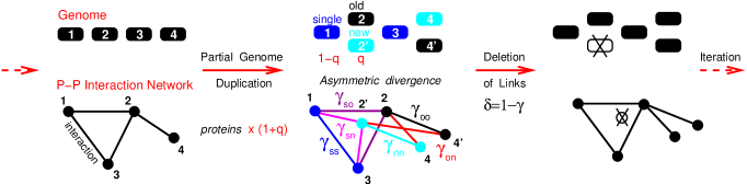
Figure 1: General Duplication-Divergence Model for protein-protein interaction network evolution. Successive duplications of a fraction $q$ of genes are followed by an asymmetric divergence of gene duplicates (e.g. 2 vs $2^{\prime}$): “New” duplicates ($n$) are left essentially free to accumulate neutral mutations with the likely outcome to become nonfunctional and eventually deleted unless some “new”, duplication-derived interactions are selected; “Old” duplicates ($o$), on the other hand, are more constrained to conserve “old” interactions already present before duplication. Links on the locally ($q\ll 1$), partially ($q<1$) or fully ($q=1$) duplicated network are then preserved stochastically with different probabilities $\gamma_{ij}$ ($0\leq\gamma_{ij}\leq 1$, $i,j=s,o,n$) reflecting the recent history of each interacting partners, that are either “singular”, non-duplicated genes ($s$) or recently duplicated genes undergoing asymmetric divergence ($o/n$). The GDD model has 6 $\gamma_{ij}$ parameters, which reduce to 3 for local ($q\ll 1$) and whole genome ($q=1$) duplications (see text).

Introduction

The primary source of new protein functions is generally considered to originate from duplication of existing genes followed by functional divergence of their duplicate copies[2, 3]. In fact, duplication-divergence events occur at a wide range of genomic scales, from many independent duplications of individual genes to rare but evolutionary dramatic duplications of entire genomes. For instance, there were between 2 and 4 consecutive whole genome duplications in all major eukaryote kingdoms in the last 500MY, about 15% of life history (see refs in[4]). Extrapolating these “recent” records, one roughly expects a few tens consecutive whole genome duplications (or equivalent “doubling events”) since the origin of life[4].

Clearly, this succession of whole genome duplications, together with the accumulation of individual gene duplications, must have greatly contributed to shape the global structure of large biological networks, such as protein-protein interaction (PPI) networks, that control cellular activities.

Ispolatov et al.[5], recently proposed an interesting local duplication-divergence model of PPI network evolution based on i) natural selection at the level of individual duplication-derived interactions and ii) a time-linear increase in genome and PPI network sizes. Yet, we expect that independent local duplications and, a forceriori, partial or whole genome duplications all lead to exponential evolutionary dynamics of PPI networks (as typically assumed at the scale of entire ecosystems). In the long time limit, exponential dynamics should outweigh all time-linear processes that have been assumed in PPI network evolution models so far[6, 7, 8, 9, 10, 5, 11, 12].

This paper proposes and asymptotically solves a general duplication-divergence model based on prevailing exponential dynamics of PPI network evolution under local, partial or global genome duplications. Our aim, here, is to establish a theoretical baseline from which other evolutionary processes beyond strict duplication-divergence events, such as shuffling of protein domains[4] or horizontal gene transfers, can then be considered.

Results

General Duplication-Divergence Model

The general duplication-divergence (GDD) model is designed to capture large scale properties of PPI networks arising from statistical selection at the level of duplication-derived interactions, which we see as a spontaneous “background” dynamics for PPI network evolution.

At each time step, a fraction $q$ of extant genes is duplicated, followed by functional divergence between duplicates, Fig. 1. In the following, we first solve the GDD model assuming that $q$ is constant over evolutionary time scales. We then study more realistic scenarios combining, for instance, rare whole genome duplications ($q=1$) with more frequent local duplications of individual genes ($q\ll 1$), and including also stochastic fluctuations in all microscopic parameters of the GDD model (see Fig. 1 and below).

Natural selection is modeled statistically (i.e., regarless of specific evolutionary advantages) at the level of duplication-derived interactions. We assume that ancient and recent duplication-derived interactions are stochastically conserved after each duplication with distinct probabilities $\gamma_{ij}$’s, depending only on the recently duplicated or non-duplicated state of each protein partners, as well as on the asymmetric divergence between gene duplicates[4], see Fig. 1 caption (’$s$’ for “singular”, non-duplicated genes and ’$o$’/’$n$’ for “old”/“new” asymmetrically divergent duplicates). Hence, the GDD model depends on 1+6 parameters, i.e., $q$ plus 6 $\gamma$’s ($\gamma_{ss}$, $\gamma_{so}$ $\gamma_{sn}$, $\gamma_{oo}$, $\gamma_{on}$ and $\gamma_{nn}$). This parameter space greatly simplifies, however, for two limit evolutionary scenarios of great biological importance: i) local duplications ($q\ll 1$), controlled by $\gamma_{ss}$, $\gamma_{so}$ and $\gamma_{sn}$, and ii) whole genome duplications ($q=1$), controlled by $\gamma_{oo}$, $\gamma_{on}$ and $\gamma_{nn}$.

We study the GDD evolutionary dynamics of PPI networks in terms of ensemble averages $\langle Q^{(n)}\rangle$ defined as the mean value of a feature $Q$ over all realizations of the evolutionary dynamics after $n$ successive duplications. This does not imply, of course, that all network realizations “coexist” but only that a random selection of them are reasonably well characterized by the theoretical ensemble average. While generally not the case for exponentially growing systems, we can show, here, that ensemble averages over all evolutionary dynamics indeed reflect the properties of typical network realizations for biologically relevant regimes (see Statistical properties of GDD models in Supp. Information).

In the following, we focus the discussion on the number of proteins (or “nodes”) $N_{k}$ of connectivity $k$ in PPI networks, while postponing the analysis of GDD models for simple non-local motifs to the end of the paper and Supporting Information. The total number of nodes in the network is noted $N=\sum_{k\geq 0}N_{k}$ and the total number of interactions (or “links”) $L=\sum_{k\geq 0}kN_{k}/2$. The dynamics of the ensemble averages $\langle N_{k}^{(n)}\rangle$ after $n$ duplications is analyzed using a generating function,

$$F^{(n)}(x)=\sum_{k\geq 0}\langle N_{k}^{(n)}\rangle x^{k}.$$ (1)

The evolutionary dynamics of $F^{(n)}(x)$ correponds to the following recurrence deduced from the microscopic definition of the GDD model (see Supporting Information),

$$F^{(n+1)}(x)=(1\!-\!q)F^{(n)}\bigl{(}A_{s}(x)\bigr{)}+qF^{(n)}\bigl{(}A_{o}(x)\bigr{)}+qF^{(n)}\bigl{(}A_{n}(x)\bigr{)}$$

where we note for $i=s,o,n$,

$$A_{i}(x)=(1\!-\!q)(\gamma_{is}x+\delta_{is})+q(\gamma_{io}x+\delta_{io})(\gamma_{in}x+\delta_{in})$$

with $\gamma_{ij}=\gamma_{ji}$ and $\delta_{ij}=1-\gamma_{ij}$ corresponding to deletion probabilities ($i,j=s,o,n$). The average growth/decrease rate of connectivity $\Gamma_{i}$ for each type of nodes corresponds to $A^{\prime}_{i}(1)$ (i.e., degree $k\!\to\!k\Gamma_{i}$ on average for node $i=s,o,n$),

$$\Gamma_{i}=A^{\prime}_{i}(1)=(1\!-\!q)\gamma_{is}+q(\gamma_{io}+\gamma_{in})$$

In the following, we assume $\Gamma_{o}\geq\Gamma_{n}$ by definition of “old” and “new” duplicates due to asymmetric divergence.

Evolutionary growth and conservation of PPI network

The total number of nodes generated by the GDD model, $F^{(n)}(1)$, growths exponentially with the number of partial duplications, $F^{(n)}(1)=C\!\cdot\!(1+q)^{n}$, where $C$ is the initial number of nodes, as a constant fraction of nodes $q$ is duplicated at each time step. Yet, some nodes become completely disconnected from the rest of the graph during divergence and rejoin the disconnected component of size $F^{(n)}(0)$. From a biological point of view, these disconnected nodes represent genes that have presumably lost all biological functions and become pseudogenes before being simply eliminated from the genome. We neglect the possibility for nonfunctional genes to reconvert to functional genes again after suitable mutations, and remove them at each round of partial duplication, focussing solely on the connected part of the graph.

In particular, the link growth rate $(1-q)\Gamma_{s}+q\Gamma_{o}+q\Gamma_{n}$, obtained by taking the first derivative of (General Duplication-Divergence Model) at $x=1$, controls whether the connected part of the graph is exponentially growing ($>1$) or shrinking ($<1$).

Let us now introduce another rate of prime biological interest, $M=(1-q)\Gamma_{s}+q\Gamma_{o}$. It is the average rate of connectivity increase for the most conserved duplicate lineage, which corresponds to a stochastic alternance between singular (’$s$’) and most conserved (’$o$’) duplicate descents. Hence, $M=(1-q)\Gamma_{s}+q\Gamma_{o}$ can be seen as a network conservation index, since individual proteins in the network all tend to be conserved if $M\geq 1$, while non-conserved PPI networks arise from continuous renewing of nodes and local topologies, if $M=(1-q)\Gamma_{s}+q\Gamma_{o}<1$ (and $(1-q)\Gamma_{s}+q\Gamma_{o}+q\Gamma_{n}\geq 1$ to ensure a non-vanishing connected network). Clearly, non-vanishing and conserved graphs seem the only networks of potential biological interest (see Discussion). The resulting conditions on GDD model parameters are summarized in Fig. 2. In particular, $1\!+\!q\!-\!(1\!-\!q)^{2}(1\!-\!\gamma_{ss})>1$, implying $\gamma_{ss}>1-q$, in the local duplication limit, $q\ll 1$.

Evolution of PPI network degree distribution

In practice, we rescale the exponentially growing connected graph by introducing a normalized generating function for the average degree distribution,

$$p^{(n)}(x)=\sum_{k\geq 1}p_{k}^{(n)}x^{k}\;\;{\rm with}\;\;\;p_{k}^{(n)}={\langle N_{k}^{(n)}\rangle\over\langle N^{(n)}\rangle},$$ (2)

Figure 2: Evolutionary growth and conservation of PPI networks. Phase diagram of GDD models for local (blue, $q\ll 1$, $\gamma_{ss}=1$), partial (black, $q<1$) and whole genome (red, $q=1$) duplications, in the $\bigl{(}(1\!-\!q)\Gamma_{s}+q\Gamma_{o}+q\Gamma_{n}$, $(1\!-\!q)\Gamma_{s}+q\Gamma_{o}\bigr{)}$ plane.

where $\langle N^{(n)}\rangle=\sum_{k\geq 1}\langle N_{k}^{(n)}\rangle$, i.e. after removing $\langle N_{0}^{(n)}\rangle$.

$F^{(n)}(x)$ can be reconstructed from the shifted degree distribution, $\tilde{p}^{(n)}(x)=p^{(n)}(x)-1$, as,

$$F^{(n)}(x)=\langle N^{(n)}\rangle\tilde{p}^{(n)}(x)+C\cdot(1+q)^{n},$$ (3)

which yields the following recurrence for $\tilde{p}^{(n)}(x)$,

$$\tilde{p}^{(n+1)}(x)={(1\!-\!q)\tilde{p}^{(n)}\!\bigl{(}A_{s}(x)\bigr{)}+q\;\tilde{p}^{(n)}\!\bigl{(}A_{o}(x)\bigr{)}+q\;\tilde{p}^{(n)}\!\bigl{(}A_{n}(x)\bigr{)}\over\Delta^{(n)}}$$

where $\Delta^{(n)}$ is the ratio between two consecutive graph sizes in terms of connected nodes,

$$\Delta^{(n)}={\langle N^{(n+1)}\rangle\over\langle N^{(n)}\rangle}=-(1-q)\tilde{p}^{(n)}\bigl{(}A_{s}(0)\bigr{)}-q\;\tilde{p}^{(n)}\!\bigl{(}A_{o}(0)\bigr{)}-q\;\tilde{p}^{(n)}\!\bigl{(}A_{n}(0)\bigr{)}>0$$

While $\Delta^{(n)}$ is not known a priori and should, in general, be determined self-consistently with $\tilde{p}^{(n)}(x)$ itself, it is directly related to the evolution of the mean degree $\overline{k}^{(n)}=\sum_{k\geq 1}kp^{(n)}_{k}$ obtained by taking the first derivative of (Evolution of PPI network degree distribution) at $x=1$,

$${\overline{k}^{(n+1)}\over\overline{k}^{(n)}}={(1-q)\Gamma_{s}+q\Gamma_{o}+q\Gamma_{n}\over\Delta^{(n)}}.$$ (4)

Hence, although connected networks grow exponentially both in terms of number of links (link growth rate $(1\!-\!q)\Gamma_{s}\!+\!q\Gamma_{o}\!+\!q\Gamma_{n}$) and number of connected nodes (node growth rate $\Delta^{(n)}$), features normalized over these growing networks, such as node mean connectivity (4) or distributions of node degree (or simple non-local motifs, see below) exhibit richer evolutionary dynamics in the asymptotic limit $n\!\rightarrow\!\infty$, as we now discuss.

Asymptotic analysis of node degree distribution

The node degree distribution can be shown (see Supp. Information) to converge towards a limit function $p(x)$, with $\tilde{p}(x)=p(x)-1$ solution of the functional eq.(Evolution of PPI network degree distribution)

$$\tilde{p}(x)={(1-q)\tilde{p}\bigl{(}A_{s}(x)\bigr{)}+q\;\tilde{p}\bigl{(}A_{o}(x)\bigr{)}+q\;\tilde{p}\bigl{(}A_{n}(x)\bigr{)}\over\Delta}$$

where $\Delta=\lim_{n\rightarrow\infty}\Delta^{(n)}$ with both $\Delta\leq 1\!+\!q$, the maximum node growth rate, and $\Delta\leq(1-q)\Gamma_{s}+q\Gamma_{o}+q\Gamma_{n}$, the link growth rate, as the number of connected nodes cannot increase faster than the number of links. Asymptotic regimes with $\Delta=(1-q)\Gamma_{s}+q\Gamma_{o}+q\Gamma_{n}$ correspond to the same exponential growth of the network in terms of connected nodes and links, and will be referred to as linear regimes, hereafter, while $\Delta<(1-q)\Gamma_{s}+q\Gamma_{o}+q\Gamma_{n}$ corresponds to non-linear asymptotic regimes, which imply a diverging mean connectivity ${\overline{k}}^{(n)}\!\to\infty$ in the asymptotic limit $n\to\infty$, Eq.(4).

In order to determine $\Delta$ and $p(x)$ self-consistently, we first express successive derivatives of $p(x)$ at $x=1$ in terms of lower derivatives, using Eq.(Asymptotic analysis of node degree distribution),

$$\partial_{x}^{k}p(1)\biggl{[}1-{(1-q)\Gamma^{k}_{s}+q\Gamma^{k}_{o}+q\Gamma^{k}_{n}\over\Delta}\biggr{]}\!=\!\!\!\sum_{l=[k/2]}^{k}\!\!\!\alpha_{k,l}\;\partial_{x}^{l}p(1),$$ (5)

where $\alpha_{k,l}$ are positive functions of the 1+6 parameters. Inspection of this expression readily defines two classes of asymptotic regimes, regular and singular regimes, which can be further analyzed with the “characteristic function” $h(\alpha)=(1-q)\Gamma_{s}^{\alpha}+q\Gamma_{o}^{\alpha}+q\Gamma_{n}^{\alpha}$, as outlined below and in Fig. 3 (see Asymptotic methods in Supp. Information for proof details).

Figure 3: Asymptotic degree distribution for GDD models. Asymptotic regimes are deduced from the convex characteristic function $h(\alpha)$ and its derivatives $h^{\prime}(0)$ and $h^{\prime}(1)$ (see text).

Regular regimes, if $M^{\prime}=\max_{i}(\Gamma_{i})<1$, for $i=s,o,n$. In this case, the only possible solution is $\Delta=h(1)$ (i.e. linear regime). Hence, since $M^{\prime}<1$, $h(1)>h(k)$ and successive derivatives $\partial_{x}^{k}p(1)$ are thus finite and positive for all $k\geq 1$. This corresponds to an exponential decrease of the node degree distribution for $k\gg 1$, $p_{k}\propto e^{-\mu k}$ with a power law prefactor. The limit average connectivity (4) is finite in this case, $\overline{k}<\infty$.

Singular regimes, if $M^{\prime}=\max_{i}(\Gamma_{i})>1$, for $i=s,o,n$. In this case, Eq.(5) suggests that there exists an integer $r\geq 1$ for which the $r$th-derivative is negative, $\partial_{x}^{r}p(1)<0$, which is impossible by definition. This simply means that neither this derivative nor any higher ones exist (for $k\geq r$). We thus look for self-consistent solutions of the “characteristic equation” $h(\alpha)=\Delta$, (with $r-1<\alpha\leq r$) corresponding to a singularity of $p(x)$ at $x=1$ and a power law tail of $p_{k}$, for $k\gg 1$[13],

$$p(x)=1-\cdots-A_{\alpha}(1-x)^{\alpha}+\cdots\;{\rm and}\;\;\;p_{k}\propto k^{-\alpha-1}$$ (6)

where the singular term $(1\!-\!x)^{\alpha}$ is replaced by $(1\!-\!x)^{r}\ln(1\!-\!x)$ for $\alpha=r$ exactly. Several asymptotic behaviors are predicted from the convex shape of $h(\alpha)$ ($\partial_{\alpha}^{2}h\geq 0$), depending on the signs of its derivatives $h^{\prime}(0)$ and $h^{\prime}(1)$, Fig. 3 (inset).

• If $h^{\prime}(0)<0$ and $h^{\prime}(1)<0$. There exists an $\alpha^{\star}>1$ so that $h(\alpha^{\star})=h(1)$ and the condition $\Delta\leq h(1)$ implies $\alpha^{\star}\geq\alpha\geq 1$. The solution $\alpha=1$ requires $h^{\prime}(1)=0$ and should be rejected in this case. Hence, since $\overline{k}<\infty$ for $\alpha>1$, we must have $\Delta=h(1)$ (linear regime) and a scale-free limit degree distribution with a unique $\alpha=\alpha^{\star}\!>\!1$, $\;\;p_{k}\propto k^{-\alpha^{\star}-1}$ for $k\gg 1$.

• If $h^{\prime}(0)<0$ and $h^{\prime}(1)=0$. $\alpha=1$, $\Delta=h(1)$ and $p_{k}\propto k^{-2}$ for $k\gg 1$ ($\overline{k}^{(n)}\to\infty$ as $n\to\infty$).

• If $h^{\prime}(0)<0$ and $h^{\prime}(1)>0$. The general condition $\Delta\leq\min(h(0),h(1))$ leads a priori to a whole range of possible $\alpha\in]0,1]$ corresponding to stationary scale-free degree distributions with diverging mean degrees $\overline{k}^{(n)}\!\to\infty$. Yet, numerical simulations suggest that there might still be a unique asymptotic node growth rate $\Delta$ regardless of initial conditions or evolution trajectories, although convergence is extremely slow (See Numerical simulations in Supp. Information).

• If $h^{\prime}(0)\geq 0$ and $h^{\prime}(1)>0$. $\Delta=h(0)=1\!+\!q$ implying that all duplicated nodes are selected in this case. No suitable $\alpha$ exist as the node degree distribution is exponentially shifted towards higher and higher connectivities. This is a dense, non-stationary regime with seemingly little relevance to biological networks.

Finally, note that the characteristic equation $\Delta=h(\alpha)$ can be recovered directly from the average change of connectivity $k\to k\Gamma_{i}$ and the following continuous approximation (using $N^{(n)}\!=\!\sum_{k}N^{(n)}_{k}\!\simeq\!\int_{u}N^{(n)}_{u}du$ and $\langle N^{(n)}_{k}\rangle\!\propto\!k^{-\alpha-1}$),

$${\langle N^{(n\!+\!1)}\rangle\over\langle N^{(n)}\rangle}\!\simeq\!{\int\bigl{\langle}(1\!-\!q)N^{(n)}_{k\Gamma_{s}}\Gamma_{s}\!+\!qN^{(n)}_{k\Gamma_{o}}\Gamma_{o}\!+\!qN^{(n)}_{k\Gamma_{n}}\Gamma_{n}\bigr{\rangle}dk\over\int_{u}\langle N^{(n)}_{u}\rangle du}\!=\!h(\alpha)$$

Local and Global Duplication limits and realistic hybrid models

We focus here on the biologically relevant cases of growing, yet not asymptotically dense networks. Figs. 4A & B summarize the asymptotic evolutionary dynamics of the GDD model in two limit cases of great biological importance: i) for local duplication-divergence events ($q\ll 1$ and $\gamma_{ss}=1$, Fig. 4A) and ii) for whole genome duplication-divergence events ($q=1$, Fig. 4B), see Supp. Information for details.

The local duplication-divergence limit leads to scale-free limit degree distributions for both conserved and non-conserved networks, with power law exponents $1<\alpha+1\leq 3$ if $\gamma_{so}=1$ (i.e. which ensures that all previous interactions are conserved in at least one copy after duplication).

By contrast, the whole genome duplication-divergence limit leads to a wide range of asymptotic behaviors from non-conserved, exponential regimes to conserved, scale free regimes with arbitrary power law exponents. Conserved, non-dense networks require, however, an asymmetric divergence between old and new duplicates ($\gamma_{oo}\neq\gamma_{nn}$)[4] and lead to scale-free limit degree distributions with power law exponents $1<\alpha+1\leq 3$ for maximum divergence asymmetry ($\gamma_{oo}=1$ and $\gamma_{nn}=0$).

Figure 4: Asymptotic phase diagram of PPI networks under the GDD model. A. Local duplication-divergence limit ($q\ll 1$ and $\gamma_{ss}=1$). B. Whole genome duplication-divergence limit ($q=1$). Boxed figures are power law exponents of scale-free regimes.

We now outline the predictions for a more realistic GDD model combining $R\!-\!1\gg 1$ local duplications ($q\ll 1$) for each whole genome duplication ($q=1$). This hybrid model of PPI network evolution amounts to a simple extension of the initial GDD model with fixed $q$ (see Supp. Information).

Network conservation is now controlled by the cummulated product of connectivity growth/decrease rates over one whole genome duplication and $R\!-\!1$ local duplications, following the most conserved, “old” duplicate lineage,

$$M=\Bigl{(}\Gamma_{o}(1)\cdot\bigl{[}(1\!-\!q)\Gamma_{s}(q)+q\Gamma_{o}(q)\bigr{]}^{R-1}\Bigr{)}^{1/R}$$ (7)

where we note the explicit dependence of $\Gamma_{i}$ in $q$ ($i=s,o,n$): $\Gamma_{i}(q)=(1\!-\!q)\gamma_{is}+q(\gamma_{io}+\gamma_{in})$. Hence, conserved [resp. non-conserved] networks correspond to $M>1$ [resp. $M<1$].

A similar cummulated product also controls the effective node degree exponent $\alpha$ and node growth rate $\Delta$ which are self-consistent solutions of the characteristic equation,

$$\Bigl{(}h(\alpha,1)\cdot\bigl{[}h(\alpha,q)\bigr{]}^{R-1}\Bigr{)}^{1/R}=\Delta$$ (8)

where we note the explicit dependence of function $h(\cdot)$ for $\alpha$ and $q$: $h(\alpha,q)=(1\!-\!q)\Gamma^{\alpha}_{s}(q)+q\Gamma^{\alpha}_{o}(q)+q\Gamma^{\alpha}_{n}(q)$ as before.

Hence, the asymptotic degree distribution for the hybrid model is controlled by the parameter

$$M^{\prime}=\Bigl{(}\Gamma_{o}(1)\cdot\max_{i}\bigl{(}\Gamma^{R-1}_{i}(q)\bigr{)}\Bigr{)}^{1/R}$$ (9)

with $M^{\prime}>1$ [resp. $M^{\prime}<1$] for scale-free (or dense) [resp. exponential] limit degree distribution. In particular, assuming $\Gamma_{s}(q)\geq\Gamma_{o}(q)$, we find ${M^{\prime}}^{R}=\Gamma_{o}(1)\Gamma^{R-1}_{s}(q)$ and thus,

$${M^{\prime}}^{R}\!=\Gamma_{o}(1)\cdot{\gamma_{ss}^{R-1}\Bigl{(}1+q\bigl{(}{\gamma_{so}+\gamma_{sn}\over\gamma_{ss}}-1\bigr{)}\Bigr{)}^{R-1}}$$

$$\;\;\;\;\;\;\;\;\simeq\Gamma_{o}(1)\sqrt{[h(1,q)]^{R-1}}\;\;\;\;\;{\rm for}\;\;\;\gamma_{ss}=1,\;\;Rq^{2}\ll 1$$

The square root dependency in terms of cummulated growth rate by $R\!-\!1$ local duplications, $[h(1,q)]^{R-1}$, implies that non-conserved, exponential regimes for whole genome duplications (if $\Gamma_{o}(1)<1$) are not easily compensated by local duplications, suggesting that asymmetric divergence between duplicates is still required, in practice, to obtain (conserved) scale-free networks. In this case, the asymptotic exponent of the hybrid model $\alpha_{h}$ lies between those for purely local ($\alpha_{\ell}$) and purely global ($\alpha_{g}$) duplications, that are solution of $h(\alpha_{\ell},q)=\Delta_{\ell}$ and $h(\alpha_{g},1)=\Delta_{g}$, with typical scale-free exponents $\alpha_{\ell}+1$, $\alpha_{g}+1$ and, hence, $\alpha_{h}+1\in[2,3]$, for $\overline{k}<\infty$. Analysis of available PPI data is discussed in[4].

The previous analysis can be readily extended to any duplication-divergence hybrid models with arbitrary series of the 1+6 microscopic parameters including stochastic fluctuations ${\{q^{(n)},\gamma^{(n)}_{ij}\}}_{R}\!\in\![0,1]$, for $i,j=s,o,n$. Network conservation still corresponds to the condition $M>1$, where the network conservation index now reads,

$$M=\biggl{(}\prod^{R}_{n}\Bigl{[}(1\!-\!q^{(n)})\Gamma_{s}^{(n)}+q^{(n)}\Gamma_{o}^{(n)}\Bigr{]}\biggr{)}^{1/R}$$ (10)

while the nature of the asymptotic degree distribution is controlled by,

$$M^{\prime}=\biggl{(}\prod^{R}_{n}\max_{i}\bigl{(}\Gamma_{i}^{(n)}\bigr{)}\biggr{)}^{1/R}$$ (11)

with $M^{\prime}<1$ corresponding to exponential networks and $M^{\prime}>1$ to scale-free (or dense) networks with an effective node degree exponent $\alpha$ and effective node growth rate $\Delta$ that are self-consistent solutions of the generalized characteristic equation,

$$h(\alpha)=\biggl{(}\prod^{R}_{n}h^{(n)}\bigl{(}\alpha,q^{(n)}\bigr{)}\biggr{)}^{1/R}=\Delta$$ (12)

This leads to exactly the same discussion for singular regimes as with constant $q$ and $\Gamma_{i}$ (Fig. 3) due to the convexity of the generalized function $h(\alpha)$ ($\partial^{2}_{\alpha}h(\alpha)\geq 0$, see Supp. Information for details and discussion on the $R\to\infty$ limit).

In particular, since $(1\!-\!q^{(n)})\Gamma^{(n)}_{s}+q^{(n)}\Gamma^{(n)}_{o}\leq\max_{i}\bigl{(}\Gamma^{(n)}_{i}\bigr{)}$ for all $q^{(n)}$ and $\Gamma^{(n)}_{i}$ ($i=s,o,n$), we always have $M\leq M^{\prime}$. Hence, the evolution of PPI networks under the most general duplication-divergence hybrid model implies that all conserved networks are necessary scale-free (or dense) ($1<M\leq M^{\prime}$), while all exponential networks are necessary non-conserved ($M\leq M^{\prime}<1$), see Discussion below.

Simple non-local PPI network properties

The generating function approach introduced for node degree evolution $N^{(n)}_{k}$ (Fig. 5A) can also be applied to simple motifs of PPI networks, whose evolutionary conservation is also controlled by the same general condition $M>1$ (see Discussion).

We just outline, here, the approach for two simple motifs capturing the node degree correlations between 2 interacting partners, $N^{(n)}_{k,l}$ (Fig. 5B) and 3 interacting partners (triangles), $T^{(n)}_{k,l,m}$ (Fig. 5C).

Figure 5: Simple correlation motifs in PPI networks.

The evolutionary dynamics of these correlation motifs can be described in terms of generating functions,

$$H^{(n)}(x,y) = \sum_{k\geq 0,\;l\geq 0}\langle N^{(n)}_{k,l}\rangle x^{k}y^{l},$$ (13)

$$T^{(n)}(x,y,z) = \sum_{k\geq 0,\;l\geq 0,\;m\geq 0}\langle T^{(n)}_{k,l,m}\rangle x^{k}y^{l}z^{m}$$ (14)

and rescaled generating functions,

$$h^{(n)}(x,y) = \sum_{k\geq 0,\;l\geq 0}{\langle N^{(n)}_{k,l}\rangle\over 2\langle L^{(n)}\rangle}x^{k}y^{l},$$ (15)

$$t^{(n)}(x,y,z) = \sum_{k\geq 0,\;l\geq 0,\;m\geq 0}{\langle T^{(n)}_{k,l,m}\rangle\over 6\langle T^{(n)}\rangle}x^{k}y^{l}z^{m}$$ (16)

where $\langle L^{(n)}\rangle=H^{(n)}(1,1)/2$ is the number of links and $\langle T^{(n)}\rangle=T^{(n)}(1,1,1)/6$, the number of triangles.

Linear recurrence relations similar to (General Duplication-Divergence Model) and (Evolution of PPI network degree distribution) can be written down for the generating functions $H^{(n)}(x,y)$, $T^{(n)}(x,y,z)$, $h^{(n)}(x,y)$ and $t^{(n)}(x,y,z)$ (see Supp. Information). These relations capturing all correlations between 2 or 3 directly interacting partners can also be used to deduce simpler and more familiar network features such as the distributions of neighbour average connectivity $g(k)$[14, 15] and clustering coefficient $C(k)$[16, 17], defined as,

$$g^{(n)}(k)={\sum_{l\geq 0}(l+1)\langle N_{k-1,l}^{(n)}\rangle\over k\langle N_{k}^{(n)}\rangle}={\partial^{k-1}_{x}h^{(n)}_{1}(x)|_{x=0}\over\partial^{k-1}_{x}h^{(n)}_{0}(x)|_{x=0}}+1$$ (17)

with $h^{(n)}_{0}(x)=\partial_{y}h^{(n)}(x,y)|_{y=1},\;\;h^{(n)}_{1}(x)=h^{(n)}(x,1)$ and,

$$C^{(n)}(k) = {\sum_{l\geq 0,\;m\geq 0}\langle T^{(n)}_{(k-2,l,m)}\rangle\over k(k-1)\langle N^{(n)}_{k}\rangle}$$ (18)

$$= {6\langle T^{(n)}\rangle\over k(k-1)\langle N^{(n)}\rangle}{\partial_{x}^{k-2}t_{0}^{(n)}(x)|_{x=0}\over\partial_{x}^{k}p^{(n)}(x)|_{x=0}},$$

where $t_{0}^{(n)}(x)=t^{(n)}(x,1,1)$ and $6\langle T^{(n)}\rangle=t_{0}^{(n)}(1)$.

Discussion

We showed that general duplication-divergence processes can lead, in principle, to a broad variety of local and global topologies for conserved and non-conserved PPI networks. These are generic properties of GDD models, which are largely insensitive to intrinsic fluctuations of any microscopic parameters.

Non-conserved networks emerge when most nodes disappear exponentially fast, over evolutionary time scales, and with them all traces of network evolution. The network topology is not preserved, but instead continuously renewed from duplication of the (few) most connected nodes.

By contrast, conserved networks arise if (and only if) extant proteins statistically keep on increasing their connectivity once they have emerged from a duplication-divergence event. This implies that most proteins and their interaction partners are conserved throughout the evolution process, thereby ensuring that local topologies of previous PPI networks remain typically embedded in subsequent PPI networks. Clearly, conserved, non-dense networks are the sole networks of potential biological relevance arising through general duplication-divergence processes. Such PPI networks are also shown to be necessary scale-free (that is, regardless of other evolutionary advantages or selection drives than simple conservation of duplication-derived interactions).

Supporting Information

1 Proof of the evolutionary recurrence for the node degree generating function (Eq. 2)

The generating function for node degrees $N_{k}^{(n)}$ after $n$ duplications is defined as,

$$F^{(n)}(x)=\sum_{k\geq 0}\langle N_{k}^{(n)}\rangle x^{k}.$$ (19)

where $\langle\cdot\rangle$ corresponds to the ensemble average over all possible trajectories of the evolutionary dynamics. The $x^{k}$ term of $F^{(n)}(x)$ “counts” the statistical number of nodes with exactly $k$ links (one $x$ per link).

At each time step $n\to n+1$, each node can be either duplicated with probability $q$, giving rise to two node copies, or non-duplicated with probability $1-q$. Hence, in the general case with asymmetric divergence of duplicates (with a more conserved, “old” copy and a more divergent, “new” copy), there are 3 $F^{(n)}\bigl{(}A_{i}(x)\bigr{)}$ contributions to the updated $F^{(n+1)}(x)$ coming from each node type, $i=s,o,n$, for singular nodes, old and new duplicates,

$$F^{(n+1)}(x)=(1\!-\!q)F^{(n)}\bigl{(}A_{s}(x)\bigr{)}+qF^{(n)}\bigl{(}A_{o}(x)\bigr{)}+qF^{(n)}\bigl{(}A_{n}(x)\bigr{)}$$

where the substitutions $x\to A_{i}(x)$ in each $F^{(n)}$ terms ($i=s,o,n$) should reflect the statistical fate of a particular link “$x$” between a node of type $i$ and a neighbor node which is either singular ($s$) with probability $1\!-\!q$ or duplicated ($o/n$) with probability $q$. In practice, the duplication of a fraction $q$ of (neighbor) nodes first leads to the replacement $x\rightarrow(1\!-\!q)x+qx^{2}$ corresponding to the maximum preservation of links for both singular ($x$) and duplicated $o/n$ ($x^{2}$) neighbors, and then to the subtitution $x\rightarrow\gamma_{ij}x\!+\!\delta_{ij}$ for each type of neighbor nodes $j=s,o,n$ where $\gamma_{ij}$ is the probability to preserve a link “$x$” (and $\delta_{ij}=1\!-\!\gamma_{ij}$ the probability to erase it). Hence, the complete substitution correponding to the GDD model reads $x\rightarrow(1\!-\!q)(\gamma_{is}x+\delta_{is})+q(\gamma_{io}x+\delta_{io})(\gamma_{in}x+\delta_{in})=A_{i}(x)$ for $i=s,o,n$, leading to (1).

2 Statistical properties of the model

The approach we use to study the evolution of PPI networks under general duplication-divergence processes is based on ensemble averages over all evolutionary trajectories. We characterize, in particular, PPI network evolution in terms of average number of nodes and links and average degree distribution. Yet, in order for these average features to be representative of typical network dynamics, statistical fluctuations around the mean trajectory should not be too large. In practice, it means that the relative variance $\chi_{Q}^{2}(n)$ for a feature $Q^{(n)}$ should not diverge in the limit $n\rightarrow\infty$,

$${\chi_{Q}^{2}}^{(n)}=\biggl{(}{\langle Q^{2}\rangle-\langle Q\rangle^{2}\over\langle Q\rangle^{2}}\biggr{)}^{(n)}<\infty\;\;\;{\rm as}\;\;\;n\rightarrow\infty$$

and more generally the $p$th moment of $Q^{(n)}$ should not diverge more rapidly than the $p$th power of the average. If it is not the case, successive moments exhibit a whole multifractal spectrum and ensemble averages do not represent typical realizations of the evolutionary dynamics. In order to check whether it is or not the case here for general duplication-divergence models, we proceed by analyzing the probability distributions for the number of links and nodes.

The number of link $L$ has a probability distribution ${\cal P}(L)$ whose generating function ${\cal P}(x)=\sum_{L\geq 0}{\cal P}(L)x^{L}$ satisfies

$${\cal P}^{(n+1)}(x)={\cal P}^{(n)}[a(x)],$$ (20)

$$a(x)=(1-q)^{2}(\gamma_{ss}x\!+\!\delta_{ss})+2q(1-q)(\gamma_{so}x\!+\!\delta_{so})(\gamma_{sn}x\!+\!\delta_{sn})+q^{2}(\gamma_{oo}x\!+\!\delta_{oo})(\gamma_{nn}x\!+\!\delta_{nn})(\gamma_{on}x\!+\!\delta_{on})^{2}.$$

This relation can be justified in a way similar to that of the fundamental evolutionary recurrence above: each node of the initial graph will be either duplicated $d$ with probability $q$ or kept singular $s$ with probability $1-q$, leading to three possible node combinations for each link: $s-s$ link with probability $(1-q)^{2}$, $s-d$ or $d-s$ links with probability $2q(1-q)$ and $d-d$ link with probability $q^{2}$. Then each $s-s$ link is either kept with $\gamma_{ss}$ and erased with $\delta_{ss}$ leading to the substitution $x\rightarrow\gamma_{ss}x\!+\!\delta_{ss}$ in the corresponding term; each $s-d$ or $d-s$ link can lead to two links between $s$ and each $o/n$ duplicate, i.e. $x\rightarrow(\gamma_{so}x\!+\!\delta_{so})(\gamma_{sn}x\!+\!\delta_{sn})$, while each $d-d$ link can lead up to 4 links after duplication, i.e. $x\rightarrow(\gamma_{oo}x\!+\!\delta_{oo})(\gamma_{nn}x\!+\!\delta_{nn})(\gamma_{on}x\!+\!\delta_{on})^{2}$. Combining all these operations eventually yields equation (20).

Successive moments of this distribution are obtained taking successive derivatives of (20),

$$A_{k}^{(n)}={\partial_{x}^{k}}{\cal P}^{(n)}(x)\bigr{|}_{x=1},$$ (21)

and lead to the following recurrence relations

$$A_{k}^{(n+1)}=[h(1)]^{k}A_{k}^{(n)}+\frac{C}{2}k(k-1)[h(1)]^{k-2}A_{k-1}^{(n)}+\ldots$$

where $h(1)=a^{\prime}(1)=(1-q)\Gamma_{s}\!+\!q\Gamma_{o}\!+\!q\Gamma_{n}$ and $C=a^{\prime\prime}(1)$ are constants depending on microscopic parameters. These relations can be solved to get the leading order behavior of successive moments

$$A_{k}^{(n)}=\tilde{A}_{k}[h(1)]^{kn}\biggl{(}1+{\cal{O}}\bigl{(}[h(1)]^{-n}\bigr{)}\biggr{)},$$ (22)

where $\tilde{A}_{k}$ are some functions of microscopic parameters.

The latter relation implies that the $k$th moment is equal (modulo some finite constant) to the $k$th power of the first moment in the leading order when $n\rightarrow\infty$. This suggests that in this limit the probability distribution should take a scaling form,

$${\cal P}^{(n)}(L)\simeq{1\over\langle L^{(n)}\rangle}{\cal{F}}\biggl{(}{L\over\langle L^{(n)}\rangle}\biggr{)},\;\;n\gg 1.$$ (23)

This hypotesis can be verified directly from the explicit form of (20)(see Appendix A for details).

Although we are not able to determine the scaling function $\cal{F}$ from previous considerations, we can derive some of its properties from the successive moments (21): in particular for $n\gg 1$ the link distribution and the function $\cal{F}$ do not present a vanishing width around their mean value but instead a finite limit width corresponding to a finite relative variance,

$${\chi^{2}_{L}}^{(n)}=\biggl{(}{\langle L^{2}\rangle-\langle L\rangle^{2}\over\langle L\rangle^{2}}\biggr{)}^{(n)}\rightarrow{1\over L^{(0)}}\biggl{(}{a^{\prime\prime}(1)\over a^{\prime}(1)(a^{\prime}(1)-1)}-1\biggr{)}<\infty,$$

This relation is found solving explicitly (21) for $k=1$ and $k=2$ given the initial number of links $L^{(0)}$. Hence, although fluctuations in the number of links are important, they remain of the same order of magnitude as the mean value. This result is in fact rather surprising for a model which clearly exhibits a memory of its previous evolutionary states and might, in principle, develop diverging fluctuations in the asymptotic limit.

Fluctuations for the total number of nodes, $N^{(n)}$, and the number of nodes of degree $k\geq 1$, $N_{k}^{(n)}$, can also be evaluated using the previous result on link fluctuations and the double inequality $N_{k}\leq N\leq 2L$, valid for any graph realization. Indeed, we obtain the following relations between the $p$th moments and the $p$th power of the corresponding first moments,

$$\langle(N^{p})^{(n)}\rangle\leq 2^{p}\langle(L^{p})^{(n)}\rangle\propto 2^{p}\langle L^{(n)}\rangle^{p}=\bigl{(}\overline{k}^{(n)}\bigr{)}^{p}\langle N^{(n)}\rangle^{p},$$

$$\langle(N_{k}^{p})^{(n)}\rangle\leq 2^{p}\langle(L^{p})^{(n)}\rangle\propto 2^{p}\langle L^{(n)}\rangle^{p}=\bigl{(}\overline{k}^{(n)}\bigr{)}^{p}\langle N^{(n)}\rangle^{p}=\biggl{(}{\overline{k}^{(n)}\over p^{(n)}_{k}}\biggr{)}^{p}\langle N_{k}^{(n)}\rangle^{p}.$$

using $\langle L^{(n)}\rangle=\overline{k}^{(n)}\langle N^{(n)}\rangle$ and $\langle N_{k}^{(n)}\rangle=p^{(n)}_{k}\langle N^{(n)}\rangle$, for all $n\geq 1$ and $k\geq 1$. Hence, we find that fluctuations for both $N$ and $N_{k}$ remain finite in the asymptotic limit for linear asymptotic regimes corresponding to exponential or scale-free degree distributions with finite limit values for both mean degree, $\overline{k}^{(n)}\to\overline{k}<\infty$ and degree distribution $p^{(n)}_{k}\to p_{k}>0$, for all $k\geq 1$. This corresponds presumably to the most biologically relevant networks. On the other hand, for non-linear (scale-free or dense) asymptotic regimes previous arguments do not apply as $\overline{k}^{(n)}\to\infty$ (and $p_{k}^{(n)}\to 0$ for dense regime) when $n\to\infty$. The numbers of nodes $N^{(n)}$ and $N_{k}^{(n)}$ grow exponentially more slowly than the number of links $L^{(n)}$ in this case, and the growth process might develop, in principle, diverging fluctuations as compared to their averages, $\langle N^{(n)}\rangle$ and $\langle N_{k}^{(n)}\rangle$, respectively. Yet, numerical simultations (see section 8 below) tend to show that it is actually not the case, suggesting that the ensemble average approach we have used to study the GDD model is still valid for non-linear asymptotic regimes.

3 Asymptotic methods

In this section, we give more details about the asymptotic analysis of node degree distribution defined by the recurrence relation on its normalized generating function $p^{(n)}(x)$ (Evolution of PPI network degree distribution).

First of all, the series of $p^{(n)}(x)$ can be shown to converge at each point at least for some initial conditions. Indeed, let us introduce a linear operator $\cal{M}$ defined on functions continous on $[0,1]$ and acting according to (Evolution of PPI network degree distribution), i.e., $p^{(n+1)}={\cal{M}}p^{(n)}$. For two non-negative functions $f(x)$ and $g(x)$ so that $f(0)=0$, $g(0)=0$, $f(1)=1$ and $g(1)=1$, we have,

$$\forall x\in[0,1]\;\;f(x)\leq g(x)\Rightarrow\forall x\in[0,1]\;\;({\cal{M}}f)(x)\leq({\cal{M}}g)(x).$$ (24)

It can be verified that if $p^{(0)}(x)\!=\!x$ (one simple link as initial condition), ${\cal{M}}p^{(0)}(x)\!\leq\!p^{(0)}(x)\;\forall x\in[0,1]$ and by consequence, when applying ${\cal{M}}^{n}$ to this inequality, the following holds

$$0\leq p^{(n+1)}(x)\leq p^{(n)}(x),\;\;\forall x\in[0,1]$$

which means that at each point the series of $p^{(n)}(x)$ is decreasing and converges to some non-negative value $p(x)$. Futhermore, numerical simulations show that for an arbitrary initial condition, there exists an $n_{0}>1$ suffisiently large so that $p^{(n)}(x)$ decreases for $n\geq n_{0}$. Hence, we can take the limit $n\rightarrow\infty$ on both sides of (Evolution of PPI network degree distribution) to get the equation (Asymptotic analysis of node degree distribution) for the limit function $p(x)$.

We analyze the properties of this generating function $p(x)$ for the limit degree distribution, using asymptotic methods. Indeed, we have no mean to solve analytically this functional equation to precisely obtain the corresponding limit degree distribution, but we have enough information to deduce its asymptotic behavior at large $k$, since it is directly related to the asymptotic properties of $p(x)$ for $x\rightarrow 1$. In the following, we note $h(\alpha)=(1-q)\Gamma_{s}^{\alpha}+q\Gamma_{o}^{\alpha}+q\Gamma_{n}^{\alpha}$, following the same notation as in the main text.

First, we consider the relation between successive derivatives of $p(x)$ at $x=1$ deduced from (Evolution of PPI network degree distribution) by taking the corresponding number of derivatives, eq.(5),

$$\biggl{[}1-{h(k)\over\Delta}\biggr{]}\partial_{x}^{k}p(1)\!=\!\!\!\sum_{l=[k/2]}^{k}\!\!\!\alpha_{k,l}\;\partial_{x}^{l}p(1),$$ (25)

with some positif coefficients $\alpha_{k,l}$. The value of $\Delta$ in this relation is still unknown and should be determined self-consistently with $p(x)$. Each of these derivatives can also be obtained as a limit of value $\partial_{x}^{k}p(1)=\lim_{n\rightarrow\infty}\partial_{x}^{k}p^{(n)}(1)$, with the following recurrence relation for $\partial_{x}^{k}p^{(n)}(1)=m_{k}^{(n)}$

$$m_{k}^{(n+1)}={h(k)\over\Delta^{(n)}}m_{k}^{(n)}+\frac{\tilde{C}}{2}k(k-1){h(k-2)\over\Delta^{(n)}}m_{k-1}^{(n)}+\ldots$$ (26)

directly derived from (Evolution of PPI network degree distribution). Different regimes can be identified depending on the general convex shape of $h(\alpha)$ ($\partial^{2}_{\alpha}h(\alpha)\geq 0$).

Regular regimes - $h(\alpha)$ strictly decreasing for $\alpha>0$ iff $M^{\prime}=\max_{i}(\Gamma_{i})<1$, for $i=s,o,n$.
In this case, if we suppose that $p^{\prime}(1)$ is finite, all the derivatives of $p(x)$ at $x=1$ are finite since $\Delta=h(1)$ and $h(k)<h(1)$ for $\forall k\geq 2$. In fact, the alternative situation $p^{\prime}(1)=\infty$ and $\Delta<h(1)$ is not possible as it would imply that some first moments in (26), at least $m_{1}^{(n)}$ and $m_{2}^{(n)}$, would diverge exponentially as $(h(1)/\Delta)^{n}$. However, since $h(k)<h(1)$ for $k\geq 2$, this would contradict the fact that the $n$th moment grows more rapidly than the $n$th power of the first one. Hence, we must have $\Delta=h(1)$ and the solution is not singular at $x=1$ but may have a singularity at some $x_{0}>1$.

Taking an anzats for the asymptotic expansion in the form

$$p(x)=A_{0}-A_{1}(x_{0}-x)+A_{2}(x_{0}-x)^{2}+A_{\alpha}(x_{0}-x)^{\alpha}+{\cal{O}}\bigl{(}(x_{0}-x)^{\alpha+1}\bigr{)}.$$ (27)

and inserting it in (Asymptotic analysis of node degree distribution) we find that, in order to have the singularity at $x=x_{0}$ present on both sides of the equation, $x_{0}$ has to be chosen as the root closest to 1 in the following three equations,

$$A_{s}(x)=x,\;A_{o}(x)=x,\;A_{n}(x)=x,$$ (28)

where, $A_{i}(x)=(1\!-\!q)(\gamma_{is}x+\delta_{is})+q(\gamma_{io}x+\delta_{io})(\gamma_{in}x+\delta_{in})$ for $i=s,o,n$, or explicitly (since the second root is always 1)

$$x_{0}=\min\biggl{(}{(1-q)\delta_{ss}+q\delta_{so}\delta_{sn}\over q\gamma_{so}\gamma_{sn}},{(1-q)\delta_{so}+q\delta_{oo}\delta_{on}\over q\gamma_{oo}\gamma_{on}},{(1-q)\delta_{sn}+q\delta_{on}\delta_{nn}\over q\gamma_{on}\gamma_{nn}}\biggr{)}.$$

Since $h(\alpha)$ is strictly decreasing when $\Gamma_{s}<1$, $\Gamma_{o}<1$ and $\Gamma_{n}<1$, it is straightforward to prove that all three values are greater than one, and hence, $x_{0}>1$ for regular regimes.

The value of $\alpha$ is obtained from the same equation (Evolution of PPI network degree distribution) by comparing the coefficients in front of the singular terms when developping each term near $x=x_{0}$

$$\alpha={\ln(\epsilon_{i}\Delta)\over\ln(2-\Gamma_{i})},$$ (29)

where $i=s$, $o$ or $n$ if $x_{0}$ is the solution of $A_{i}(x)=x$, $\epsilon_{s}=(1-q)^{-1}$, $\epsilon_{o}=\epsilon_{n}=q^{-1}$, and replacing also $\epsilon_{i}\rightarrow 1/2\epsilon_{i}$ or $1/3\epsilon_{i}$ if two or all three $\Gamma_{i}$’s happen to be equal, respectively.

We recall that for $h(\alpha)$ under consideration $\overline{k}=p^{\prime}(1)$ is finite and $\Delta=h(1)$. Therefore, in this regime the asymptotic growth of the graph is exponential with respect to the number of links and the number of nodes with a common growth rate $\Delta=h(1)$. We call this asymptotic behavior “linear” because $\langle L^{(n)}\rangle$ and $\langle N^{(n)}\rangle$ are asymptotically proportional.

The decrease of the limit degree distribution for $k\gg 1$ is given by [13]

$$p_{k}\propto k^{-\alpha-1}x_{0}^{-k}\biggl{(}1+{\cal{O}}\biggl{(}{1\over k}\biggr{)}\biggr{)},\;\;k\gg 1$$ (30)

and is thus exponential with a power law prefactor. When one of the $\Gamma_{i}$’s tends to one, simultaneously $x_{0}\rightarrow 1$ and $\alpha\rightarrow\infty$ and, as we will see below, we meet the singular scale-free regime for the limit mean degree distribution.

The emergence of an exponential tail for $p_{k}$ when $k\gg 1$ naturally comes from the fact that at each duplication step the probability for a node to duplicate one of its links (keeping both the original link and its copy), $q\gamma_{oo}\gamma_{on}$ for $o$ nodes, $q\gamma_{so}\gamma_{sn}$ for $s$ nodes and $q\gamma_{on}\gamma_{nn}$ for $n$ nodes, is smaller than the corresponding probabilities to delete the initial link, $(1\!-\!q)\delta_{so}+q\delta_{oo}\delta_{on}$, $(1\!-\!q)\delta_{ss}+q\delta_{so}\delta_{sn}$ and $(1\!-\!q)\delta_{sn}+q\delta_{on}\delta_{nn}$ (it is in fact equivalent to $x_{0}>1$). For this reason at each duplication only few nodes are preserved and they keep only few of their links, the graph contains many small components and has no memory about previous states. In a different way, we can develop this argument in terms of a particular node degree evolution. When $\Gamma_{o}<1$, $\Gamma_{s}<1$ and $\Gamma_{n}<1$, nodes $o$ and $s$ as well as their copies $n$ loose links in proportion to their connectivities. It means that the number of nodes of a given connectivity is modified by a Poissonian prefactor, representing the overall tendency to follow an exponentially decreasing distribution for large number of duplications.

Singular regimes - $h(\alpha)$ has a minimum on $\alpha>0$ iff $M^{\prime}=\max_{i}(\Gamma_{i})>1$, for $i=s,o,n$.
In this case, from (25) we can be sure to have a negative value for some derivative: since $h(\alpha)$ has a unique minimum, there exists an integer $r\geq 1$ so that $h(r)<\Delta<h(r+1)$ implying that $\partial_{x}^{r+1}p(1)<0$ which is impossible by construction. In fact, this indicates the presence of an irregular term in the development of $p(x)$ in the vicinity of $x=1$, and for this reason the function itself is $r$ times differentiable at this point while its $(r+1)$th and following derivatives do not exist. Hence, we take an anzats for $p(x)$ in the neighborhood of $x=1$ using the following form

$$p(x)=1-A_{1}(1-x)+A_{2}(1-x)^{2}+A_{\alpha}(1-x)^{\alpha}+{\cal{O}}\bigl{(}(1-x)^{\alpha+1}\bigr{)}$$ (31)

A priori, we do not know the exact value of $\Delta$, and it is to be determined self-consistently with $p(x)$. We then substitute (31) into (Asymptotic analysis of node degree distribution) to get a “characteristic” equation relating $\alpha$ and $\Delta$,

$$h(\alpha)=(1-q)\Gamma_{s}^{\alpha}+q\Gamma_{o}^{\alpha}+q\Gamma_{n}^{\alpha}=\Delta.$$ (32)

If we find a nontrivial value of $\alpha^{*}>0$ that are solutions of this equation, it will give us an asymptotic expression for the coefficients of the generating function of the scale free form

$$p_{k}\propto k^{-\alpha^{*}-1}\biggl{(}1+{\cal{O}}\biggl{(}{1\over k}\biggr{)}\biggr{)},\;\;k\gg 1.$$ (33)

Note that when the solution takes an integer value $\alpha^{*}=r\geq 1$ the form of the asymptotic expansion should differ from (31) because formally it is not longer singular in this case. In fact, in the anzats a logarithmic prefactor should be added in the singular term

$$p(x)=1-A_{1}(1-x)+A_{2}(1-x)^{2}+\ldots+A_{r}(1-x)^{r}+\tilde{A}_{r}(1-x)^{r}\ln(1-x)+{\cal{O}}\bigl{(}(1-x)^{r+1}\bigr{)}$$ (34)

In order for this asymptotic expansion to satisfy equation (Asymptotic analysis of node degree distribution), we should have $h(r)=\Delta$, as before, as well as an additional condition for $r=1$ namely $h^{\prime}(1)=0$.

Note also, that the characteristic equation $h(\alpha)=\Delta$ can be recovered directly (although less rigorously) using the connectivity change $k\to k\Gamma_{i}$ on average for $i$-type of nodes ($i=s,o,n$) at each duplication and the following continuous approximation, $N^{(n)}\!=\!\sum_{k}N^{(n)}_{k}\!\simeq\!\int_{u}N^{(n)}_{u}du$,

$$\Delta\!=\!{\langle N^{(n\!+\!1)}\rangle\over\langle N^{(n)}\rangle}\!\simeq\!{\int_{k}\bigl{\langle}(1\!-\!q)N^{(n)}_{k\Gamma_{s}}\Gamma_{s}\!+\!qN^{(n)}_{k\Gamma_{o}}\Gamma_{o}\!+\!qN^{(n)}_{k\Gamma_{n}}\Gamma_{n}\bigr{\rangle}dk\over\int_{u}\langle N^{(n)}_{u}\rangle du}\!=\!{\bigl{(}(1\!-\!q)\Gamma^{\alpha}_{s}\!+\!q\Gamma^{\alpha}_{o}\!+\!q\Gamma^{\alpha}_{n}\bigr{)}\int_{u}\langle N^{(n)}_{u}\rangle du\over\int_{u}\langle N^{(n)}_{u}\rangle du}\!=\!h(\alpha)$$

where we assumed that $\langle N^{(n)}_{k}\rangle\!\propto\!k^{-\alpha-1}$.

Three cases should now been distinguished depending on the signs of $h^{\prime}(0)$ and $h^{\prime}(1)$ (see Fig. 3 in main text):

1. $h^{\prime}(0)<0$ and $h^{\prime}(1)<0$.

Since $h(\alpha)\!>\!h(1)$ for $\alpha<1$, any solution of (32) has to be greater than one (as $\Delta\leq h(1)$) which implies, by vertue of (33), $\overline{k}\!<\!\infty$ and consequently $\Delta=h(1)$ exactly (which is consistent with previous considerations). So, for the parameters satisfying $h^{\prime}(1)<0$ the value of $\alpha$ we are looking for is the unique solution, $\alpha^{\star}>1$, of

$$h(\alpha^{\star})=(1\!-\!q)\Gamma^{\alpha^{\star}}_{s}\!+\!q\Gamma^{\alpha^{\star}}_{o}\!+\!q\Gamma^{\alpha^{\star}}_{n}=(1\!-\!q)\Gamma_{s}\!+\!q\Gamma_{o}\!+\!q\Gamma_{n}=h(1)$$ (35)

The other solution $\alpha=1$ should be discarded here as it corresponds to a solution only if $h^{\prime}(1)=0$ (see proof for the most general dupication-divergence hybrid models, below).

Evidently, in this regime there exists an entier $k_{0}\geq 1$ for which

$$h(k_{0})<h(\alpha^{*})\leq h(k_{0}+1),$$

and so all the derivatives of $p^{(k)}(1)$ are finite for $k\geq k_{0}$ while all following derivatives are infinite. Finally, when we fix $\Gamma_{i}$ which are less than one and make other $\Gamma_{i}\rightarrow 1$ the value of $\alpha^{*}$ tends to infinity, the scale free regime (33) meets the exponential one (30).

2. $h^{\prime}(0)<0$ and $h^{\prime}(1)\geq 0$.

The condition $\Delta\leq h(1)$ implies that only solutions with $0<\alpha\leq 1$ are possible. Therefore, surely $\overline{k}=\infty$ in this case but there is no additional constraints a posteriori on $\Delta$ which might take, in principle, a whole range of possible values between $\min_{\alpha}(h(\alpha))$ and $\min(h(0),h(1))$. Yet, numerical simulations suggest that there might still be a unique asymptotic node growth rate $\Delta$ regardless of initial conditions or evolution trajectories, although convergence is extremely slow (See Numerical simulations below).

3. $h^{\prime}(0)\geq 0$ (we always have $h^{\prime}(1)>0$ in this case).

The minimum of $h(\alpha)$ is achieved for $\alpha_{0}<0$ in this case, and $\Delta\leq 1+q\leq h(1)$. Yet because solutions of (32) cannot be negative by definition of $p(x)$, the only possibility is $\Delta=1+q$, implying that the graph grows at the maximum pace. From the point of view of the graph topology, it means that the mean degree distribution is not stationnary and for any fixed $k$ the mean fraction of nodes with this connectivity $k$ tends to zero when $n\rightarrow\infty$, the number of links grows too rapidly with respect to the number of nodes so that the graph gets more and more dense. For this reason, we refer at this regime as the dense one.

4 Whole genome duplication-divergence model ($q=1$)

The case $q=1$ describes the situation for which the entire genome is duplicated at each time step, corresponding to the evolution of PPI networks through whole genome duplications, as discussed in ref.[4]. All results obtained above in the general case remain valid although there are now no more “singular” genes ($s$) and thus no $\gamma_{ij}$’s involving them. We just summarize these results here adopting the notations of ref.[4] for the only 3 relevant $\gamma_{ij}$’s left: $\gamma_{o}\equiv\gamma_{oo}$, $\gamma_{n}\equiv\gamma_{nn}$ and $\gamma\equiv\gamma_{on}$, hence

$$\Gamma_{o}=\gamma_{o}+\gamma,\;\;\Gamma_{n}=\gamma_{n}+\gamma,$$ (36)

The model analysis then yields three different regimes (we do not consider the case $\Gamma_{o}\!+\!\Gamma_{n}<1$ for which graphs vanish)

1. Exponential regime $\Gamma_{o}\!+\!\Gamma_{n}>1$, $\max(\Gamma_{o},\Gamma_{n})<1$. The limit degree distribution is nontrivial and decreases like (30) with

$$x_{0}=\left\{\begin{array}[]{l}{\delta_{o}\delta/\gamma_{o}\gamma},\;\Gamma_{o}<\Gamma_{n}\\ {\delta_{n}\delta/\gamma_{n}\gamma},\;\Gamma_{o}\geq\Gamma_{n}\end{array}\right.$$ (37)

and

$$\alpha={\ln(\Gamma_{o}+\Gamma_{n})\over\ln\bigl{(}2-\max(\Gamma_{o},\Gamma_{n})\bigr{)}},\;\Gamma_{o}\neq\Gamma_{n}$$ (38)

while

$$\alpha={\ln(\Gamma_{o})\over\ln(2-\Gamma_{o})},\;\;{\rm for}\;\;\Gamma_{o}=\Gamma_{n}.$$ (39)

The rate of graph growth in number of nodes as well as in number of links is $\Delta=\Gamma_{o}\!+\!\Gamma_{n}$

2. Scale free regime ($\Gamma_{o}>1$, $\Gamma_{n}<1$) or ($\Gamma_{o}<1$, $\Gamma_{n}>1$). The limit degree distribution is surely nontrivial for

$$h^{\prime}(1)=\Gamma_{o}\ln\Gamma_{o}+\Gamma_{n}\ln\Gamma_{n}<0,$$ (40)

and described by an asymptotic formula (33) with $\alpha^{*}>1$ solution of

$$\Gamma_{o}^{\alpha}+\Gamma_{n}^{\alpha}=\Gamma_{o}+\Gamma_{n},$$ (41)

In this case the ratio of two consecutive sizes is also $\Delta=\Gamma_{o}\!+\!\Gamma_{n}$. When

$$h^{\prime}(1)=\Gamma_{o}\ln\Gamma_{o}+\Gamma_{n}\ln\Gamma_{n}>0,\;\;\Gamma_{o}\Gamma_{n}<1\;\;(h^{\prime}(0)<0),$$

the mean degree distribution is still expected to converge to a nontrivial asymptotically scale-free distribution with $0\leq\alpha\leq 1$.

3. Dense regime $\Gamma_{o}\Gamma_{n}>1$ (i.e. $h^{\prime}(0)>0$). The mean degree distribution is not stationary: the growing graphs get more and more dense in the sense that the fraction of nodes with an arbitrary fixed connectivity tends to zero when $n\rightarrow\infty$. Almost all new nodes are kept in the duplicated graph $\Delta=1+q$.

Because all these regimes are defined in terms of two independent parameters (instead of three), the model phase diagram can be drawn in a plane $(\Gamma_{o},\Gamma_{n})$, or equivalently in $(\Gamma_{o}\!+\!\Gamma_{n},\Gamma_{o}\!)$ (See Fig. 4B). This last representation is adapted to show explicitly the domains of node conservation and graph growth, while the alternative choice $(\Gamma_{o}\!+\!\Gamma_{n},\Gamma_{o}\!-\!\Gamma_{n})$ used in ref.[4] is best suited to illustrate the asymmetric divergence requirement to obtained scale-free networks (see [4] for a detailed discussion).

5 Local duplication-divergence limit ($q\to 0$)

A different limit model is obtained for $q$ going to zero when the mean size of the graph tends to infinity. In principle, the most general model of this kind is the one defined by a monotonous decreasing function $q(\langle N\rangle)$ with

$$\lim_{x\rightarrow\infty}q(x)=0.$$

For any function of this type, the graph growth rate in terms of links depends essentially on $\gamma_{ss}$ because

$${\langle L^{(n+1)}\rangle\over\langle L^{(n)}\rangle}=(1-q)\Gamma_{s}+q\Gamma_{o}+q\Gamma_{n}=\gamma_{ss}+2q(\gamma_{so}+\gamma_{sn}-\gamma_{ss})+{\cal{O}}(q^{2}),$$

and if $\gamma_{ss}<1$ the ensemble average of graphs will never reach infinite size, it will have at most some finite dynamics. So, we will suppose that $\gamma_{ss}=1$, to ensure an infinite growth. We remark also that $\gamma_{oo}$, $\gamma_{on}$ and $\gamma_{nn}$ appear only in the term of order $q^{2}$ in the last expression because two new nodes have to be kept in order to add any link of the type $oo$, $on$ or $nn$.

When $q$ becomes small an approximate recursion relation for generating functions can be obtained by developping (Evolution of PPI network degree distribution) (we set $\gamma_{ss}=1$) with

$$\tilde{p}^{(n)}\bigl{(}A_{s}(x)\bigr{)}=\tilde{p}^{(n)}(x)+q\bigl{(}(\delta_{so}+\gamma_{so}x)(\delta_{sn}+\gamma_{sn}x)-x\bigr{)}\partial_{x}\tilde{p}^{(n)}(x)+{\cal{O}}(q^{2})$$

$$\tilde{p}^{(n)}\bigl{(}A_{o}(x)\bigr{)}=\tilde{p}^{(n)}(\delta_{so}+\!\gamma_{so}x)+{\cal{O}}(q)$$

$$\tilde{p}^{(n)}\bigl{(}A_{n}(x)\bigr{)}=\tilde{p}^{(n)}(\delta_{sn}+\!\gamma_{sn}x)+{\cal{O}}(q)$$

, (42)

gives in linear order of $q$

$$\tilde{p}^{(n+1)}(x)={(1-q)\tilde{p}^{(n)}(x)+q\bigl{(}(\delta_{so}+\gamma_{so}x)(\delta_{sn}+\gamma_{sn}x)-x\bigr{)}\partial_{x}\tilde{p}^{(n)}(x)+q\tilde{p}^{(n)}(\delta_{so}+\!\gamma_{so}x)+q\tilde{p}^{(n)}(\delta_{sn}+\!\gamma_{sn}x)\over\Delta^{(n)}}+{\cal{O}}(q^{2})$$

with

$$\Delta^{(n)}=1-q\biggr{(}\delta_{so}\delta_{sn}\partial_{x}\tilde{p}^{(n)}(0)+\tilde{p}^{(n)}(\delta_{so})+\tilde{p}^{(n)}(\delta_{sn})-1\biggr{)},$$ (43)

an expression which does only depend on 3 of the 6 general $\gamma_{ij}$’s: $\gamma_{ss}$, $\gamma_{so}$ and $\gamma_{sn}$. By neglecting terms in $q^{2}$ we obtain a model for which duplicated nodes are completely decorrelated in the sense that the probability for an $o$ or $s$ node to have two new neighbours is zero, and consequently any two new nodes do not have common neighbors. This model can be regarded as a generalization of the local duplication model proposed in [5] for which only one node is duplicated per time step and without modification of the connectivities between any other existing nodes, i.e. $\gamma_{ss}=1$ and $\gamma_{so}=1$. Indeed, when taking for $q$ a decreasing law

$$q\bigl{(}\langle N\rangle\bigr{)}={A\over\langle N\rangle},\;\;A>0$$

on average $A$ nodes per step are duplicated. By setting $\gamma_{so}=1$ in (5) we first get the following form for the recurrence relation,

$$\tilde{p}^{(n+1)}(x)={\tilde{p}^{(n)}(x)+q\gamma_{sn}x(x-1)\partial_{x}\tilde{p}^{(n)}(x)+q\tilde{p}^{(n)}(\delta_{sn}+\!\gamma_{sn}x)\over\Delta^{(n)}},\;\;\Delta^{(n)}=1-q\tilde{p}^{(n)}(\delta_{sn}),$$ (44)

and then using the definitions of $\Delta^{(n)}$ and $p^{(n)}(x)$ (2) to reexpress it as,

$$N^{(n+1)}_{k} = N^{(n)}_{k}+A\gamma_{sn}(k-1)p^{(n)}_{k-1}-A\gamma_{sn}kp^{(n)}_{k}+A\sum_{s\geq k}C^{k}_{s}\gamma_{sn}^{k}\delta_{sn}^{s-k}p^{(n)}_{s},$$ (45)

This expression is identical to the basic recurrence relation in the model of ref.[5] for $A=1$. For an arbitrary $A$ the asymptotic properties of the growing graph are essentially the same as in ref.[5], with only the growth rate modified by a factor proportional to $A$.

In the more general cases for which both $\gamma_{sn}$ and $\gamma_{so}$ may vary (with $\gamma_{ss}=1$ remaining fix to ensure a non-vanishing graph), an asymptotic analysis can be carried out for the limit degree distribution with an asymptotic solution of the form

$$\tilde{p}(x)=-A_{1}(1-x)+A_{2}(1-x)^{2}+A_{\alpha}(1-x)^{\alpha}+{\cal{O}}\bigl{(}(1-x)^{\alpha+1}\bigr{)}$$

satisfying (5) with $q\propto A/\langle N^{(n)}\rangle$. The characteristic equation thus becomes,

$$h_{l}(\alpha)=\gamma_{so}^{\alpha}+\gamma_{sn}^{\alpha}+\alpha(\gamma_{so}+\gamma_{sn}-1)-1=\varphi,$$

where $\varphi$ is defined as

$$\varphi=\lim_{n\rightarrow\infty}{\bigl{(}\Delta^{(n)}-1)\over q^{(n)}}\;\;\Leftrightarrow\;\;\Delta^{(n)}\simeq 1+q^{(n)}\varphi,\;n\rightarrow\infty.$$

while the graph growth rate in terms of number of links is given by,

$$(1-q)\Gamma_{s}+q\Gamma_{o}+q\Gamma_{n}=1+q(2\gamma_{so}+2\gamma_{sn}-2)+{\cal{O}}(q^{2}),$$

at first order in $q$. Since the number of nodes can not grow more rapidly than the number of links, we can conclude that $\varphi\leq 2\gamma_{so}+2\gamma_{sn}-2$, in addition to, $\varphi\leq 1$, correponding to the maximum growth rate. Focussing the analysis on the case $\gamma_{so}+\gamma_{sn}>1$ for which the graph does not vanish, one finds that the “characteristic” function $h_{l}(\alpha)$ is always convex, and the following results are obtained as in the asymptotic analysis of Sec. 3 in Supp. Information:

• When $h^{\prime}_{l}(0)<0$ and $h^{\prime}_{l}(1)<0$ the characteristic equation has a solution, $\alpha^{*}>1$, and the limit degree distribution is asymptotically scale-free $p_{k}\propto k^{-\alpha^{*}-1}$ with $\alpha^{*}$ varying on the interval $[1,\infty)$ (depending on parameters $\gamma_{so}$ and $\gamma_{sn}$) while $\varphi=h_{l}(1)$.

• For $h^{\prime}_{l}(1)=0$ precisely, the singular term of the asymptotic solution becomes $(1-x)\ln(1-x)$ and the limit degree distribution decreases as $p_{k}\propto k^{-2}$, for $k\gg 1$.

• When $h^{\prime}_{l}(0)<0$ and $h^{\prime}_{l}(1)>0$, scale-free regimes with slowly decreasing degree distributions are expected in general with $\varphi\leq\min(2\gamma_{so}+\gamma_{sn}-2,1)$ and the corresponding $0<\alpha<1$.

• For $h^{\prime}_{l}(0)>0$ the mean degree distribution is not stationary, $\varphi=1$.

Fig. 4 summarizes these results for the limit degree distribution. More generally for

$$q\bigl{(}\langle N\rangle\bigr{)}={A\over\langle N\rangle^{\beta}},\;\;A>0,\;\;\beta>0,$$

when $\beta>1$, nodes a rarely duplicated so that the interval between two succesfull duplications in number of steps is approximately

$$n\propto\langle N^{(n)}\rangle^{\beta-1}.$$

Therefore $\beta>1$ gives a model equivalent to $\beta=1$ with a change of time scale. On the other hand, for $0<\beta<1$ a set of nontrivial models is obtained.

6 General duplication-divergence hybrid models

We start the analysis of GDD hybrid models with the case of two duplication-divergence steps involving some fractions $q_{1}$ and $q_{2}$ of duplicated genes, introducing explicit dependencies in $q$ and $x$ for $A_{i}(q,x)$ and $\Gamma_{i}(q)=\partial_{x}A_{i}(q,1)$ functions ($i=s,o,n$), $A_{i}(q,x)=(1\!-\!q)(\gamma_{is}x+\delta_{is})+q(\gamma_{io}x+\delta_{io})(\gamma_{in}x+\delta_{in})$ and $\Gamma_{i}(q)=(1\!-\!q)\gamma_{is}+q(\gamma_{io}+\gamma_{in})$.

An evolutionary recurrence for the hybrid generating function can be found by introducing the intermediate step explicitly, $\tilde{p}^{(n)}\rightarrow\tilde{r}^{(n)}\rightarrow\tilde{p}^{(n+1)}$ where,

$$\tilde{r}^{(n)}(x)={(1\!-\!q_{1})\tilde{p}^{(n)}\!\bigl{(}A_{s}(q_{1},x)\bigr{)}+q_{1}\;\tilde{p}^{(n)}\!\bigl{(}A_{o}(q_{1},x)\bigr{)}+q_{1}\;\tilde{p}^{(n)}\!\bigl{(}A_{n}(q_{1},x)\bigr{)}\over\Delta^{(n)}_{1}}$$

$$\Delta^{(n)}_{1}=-(1\!-\!q_{1})\tilde{p}^{(n)}\!\bigl{(}A_{s}(q_{1},0)\bigr{)}-q_{1}\;\tilde{p}^{(n)}\!\bigl{(}A_{o}(q_{1},0)\bigr{)}-q_{1}\;\tilde{p}^{(n)}\!\bigl{(}A_{n}(q_{1},0)\bigr{)}>0,$$

and then $\tilde{r}^{(n)}\rightarrow\tilde{p}^{(n+1)}$ with,

$$\tilde{p}^{(n+1)}(x)={(1\!-\!q_{2})\tilde{r}^{(n)}\!\bigl{(}A_{s}(q_{2},x)\bigr{)}+q_{2}\;\tilde{r}^{(n)}\!\bigl{(}A_{o}(q_{2},x)\bigr{)}+q_{2}\;\tilde{r}^{(n)}\!\bigl{(}A_{n}(q_{2},x)\bigr{)}\over\Delta^{(n)}_{2}}$$

$$\Delta^{(n)}_{2}=-(1\!-\!q_{2})\tilde{r}^{(n)}\!\bigl{(}A_{s}(q_{2},0)\bigr{)}-q_{2}\;\tilde{r}^{(n)}\!\bigl{(}A_{o}(q_{2},0)\bigr{)}-q_{2}\;\tilde{r}^{(n)}\!\bigl{(}A_{n}(q_{2},0)\bigr{)}>0,$$

which finally yields for the effective $\tilde{p}^{(n)}\rightarrow\tilde{p}^{(n+1)}$ step,

$$\tilde{p}^{(n+1)}(x) = {(1\!-\!q_{2})\Bigl{(}(1\!-\!q_{1})\tilde{p}^{(n)}\!\bigl{(}A_{s}(q_{1},A_{s}(q_{2},x))\bigr{)}+q_{1}\tilde{p}^{(n)}\!\bigl{(}A_{o}(q_{1},A_{s}(q_{2},x))\bigr{)}+q_{1}\tilde{p}^{(n)}\!\bigl{(}A_{n}(q_{1},A_{s}(q_{2},x))\bigr{)}\Bigr{)}\over\Delta^{(n)}_{1}\Delta^{(n)}_{2}}$$

$$+{q_{2}\Bigl{(}(1\!-\!q_{1})\tilde{p}^{(n)}\!\bigl{(}A_{s}(q_{1},A_{o}(q_{2},x))\bigr{)}+q_{1}\tilde{p}^{(n)}\!\bigl{(}A_{o}(q_{1},A_{o}(q_{2},x))\bigr{)}+q_{1}\tilde{p}^{(n)}\!\bigl{(}A_{n}(q_{1},A_{o}(q_{2},x))\bigr{)}\Bigr{)}\over\Delta^{(n)}_{1}\Delta^{(n)}_{2}}$$

$$+{q_{2}\Bigl{(}(1\!-\!q_{1})\tilde{p}^{(n)}\!\bigl{(}A_{s}(q_{1},A_{n}(q_{2},x))\bigr{)}+q_{1}\tilde{p}^{(n)}\!\bigl{(}A_{o}(q_{1},A_{n}(q_{2},x))\bigr{)}+q_{1}\tilde{p}^{(n)}\!\bigl{(}A_{n}(q_{1},A_{n}(q_{2},x))\bigr{)}\Bigr{)}\over\Delta^{(n)}_{1}\Delta^{(n)}_{2}}$$

Expressing successive derivatives at $x=1$, $\partial_{x}^{k}p(1)$, for $k\geq 2$ in the asymptotic limit ${p}^{(n)}(x)\rightarrow{p}(x)$ and $\Delta^{(n)}_{1}\Delta^{(n)}_{2}\rightarrow\Delta^{2}$ for $n\rightarrow\infty$, yields, $\partial_{x}^{k}p(1)=(1\!-\!q_{2})(1\!-\!q_{1})\Gamma_{s}^{k}(q_{2})\Gamma_{s}^{k}(q_{1})\partial_{x}^{k}p(1)+(1\!-\!q_{2})q_{1}\Gamma_{s}^{k}(q_{2})\Gamma_{o}^{k}(q_{1})\partial_{x}^{k}p(1)+\cdots$ and hence,

$$\partial_{x}^{k}p(1)\biggl{[}1-{\Bigl{(}(1-q_{1})\Gamma^{k}_{s}(q_{1})+q_{1}\Gamma^{k}_{o}(q_{1})+q_{1}\Gamma^{k}_{n}(q_{1})\Bigr{)}\Bigl{(}(1-q_{2})\Gamma^{k}_{s}(q_{2})+q_{2}\Gamma^{k}_{o}(q_{2})+q_{2}\Gamma^{k}_{n}(q_{2})\Bigr{)}\over\Delta^{2}}\biggr{]}\!=\!\!\!\sum_{l=[k/2]}^{k}\!\!\!\alpha_{k,l}\;\partial_{x}^{l}p(1),$$ (46)

In fact, this simple duplication-divergence combination can be generalized to any duplication-divergence hybrid models with arbitrary series of the 1+6 microscopic parameters ${\{q^{(n)},\gamma^{(n)}_{ij}\}}_{R}\!\in\![0,1]$, for $i,j=s,o,n$ and $1\leq n\leq R$. Each duplication-divergence step then corresponds to a different linear operator ${\cal{M}}^{(n)}$ defined by $q^{(n)}$ and the functional arguments $A_{i}^{(n)}(q^{(n)},x)=(1\!-\!q^{(n)})(\gamma^{(n)}_{is}x+\delta^{(n)}_{is})+q^{(n)}(\gamma^{(n)}_{io}x+\delta^{(n)}_{io})(\gamma^{(n)}_{in}x+\delta^{(n)}_{in})$ and $\Gamma^{(n)}_{i}=\partial_{x}A^{(n)}_{i}(q^{(n)},1)$ for $i=s,o,n$ (with $A^{(n)}_{i}(q^{(n)},1)=1$). Hence, applying the same reasoning as in Asymptotic methods to the series of linear operators ${\{{\cal{M}}^{(n)}\}}_{R}$ implies that any duplication-divergence hybrid model converges in the asymptotic limit (at least for simple initial conditions).

In the following, we first assume that the evolutionary dynamics remains cyclic with a finite period $R$, before discussing at the end the $R\to\infty$ limit, which can ultimately include intrinsic stochastic fluctuations of the microscopic parameters.

In the cyclic case with a finite period $R$, successive derivatives at $x=1$, $\partial_{x}^{k}p(1)$, can be expressed in the asymptotic limit, ${p}^{(n)}(x)\rightarrow{p}(x)$ as,

$$\partial_{x}^{k}p(1)\Biggl{(}1-{\prod^{R}_{n}\Bigl{[}(1-q^{(n)}){\Gamma_{s}^{(n)}}^{k}+q^{(n)}{\Gamma_{o}^{(n)}}^{k}+q^{(n)}{\Gamma_{n}^{(n)}}^{k}\Bigr{]}\over\Delta^{R}}\Biggr{)}\!=\!\!\!\sum_{l=[k/2]}^{k}\!\!\!\alpha_{k,l}\;\partial_{x}^{l}p(1),$$ (47)

Network conservation for such general duplication-divergence hybrid model corresponds to the condition $M>1$, where the conservation index $M$ now reads

$$M=\biggl{(}\prod^{R}_{n}\Bigl{[}(1\!-\!q^{(n)})\Gamma_{s}^{(n)}+q^{(n)}\Gamma_{o}^{(n)}\Bigr{]}\biggr{)}^{1/R}$$ (48)

while the nature of the asymptotic degree distribution is controlled by

$$M^{\prime}=\biggl{(}\prod^{R}_{n}\max_{i}\bigl{(}\Gamma_{i}^{(n)}\bigr{)}\biggr{)}^{1/R}$$ (49)

with $M^{\prime}<1$ corresponding to exponential networks and $M^{\prime}>1$ to scale-free (or dense) networks with an effective node degree exponent $\alpha$ and effective node growth rate $\Delta$ that are self-consistent solutions of the generalized characteristic equation,

$$h(\alpha)=\biggl{(}\prod^{R}_{n}h^{(n)}\bigl{(}\alpha,q^{(n)}\bigr{)}\biggr{)}^{1/R}=\Delta$$ (50)

The resolution of this generalized characteristic equation is done following exactly the same discussion for singular regimes as with constant $q$ and $\Gamma_{i}$ (Fig. 3 and main text) due to the convexity of the generalized $h(\alpha)$ function, $\partial^{2}_{\alpha}h(\alpha)\geq 0$. Indeed, the first two derivatives of $h(\alpha)$ yield (with implicit dependency in successive duplication-divergence steps, $q\equiv q^{(n)}$, $\Gamma_{i}\equiv\Gamma_{i}^{(n)}$, etc, for $i=s,o,n$),

$$\partial_{\alpha}h(\alpha) = \biggl{(}\prod^{R}_{n}h(\alpha,q)\biggr{)}^{1/R}{1\over R}\sum^{R}_{n}{\partial_{\alpha}h(\alpha,q)\over h(\alpha,q)}$$

$$= \biggl{(}\prod^{R}_{n}h(\alpha,q)\biggr{)}^{1/R}{1\over R}\sum^{R}_{n}{(1-q)\Gamma^{\alpha}_{s}\ln\Gamma_{s}+q\Gamma^{\alpha}_{o}\ln\Gamma_{o}+q\Gamma^{\alpha}_{n}\ln\Gamma_{n}\over(1-q)\Gamma^{\alpha}_{s}+q\Gamma^{\alpha}_{o}+q\Gamma^{\alpha}_{n}}$$

$$\partial^{2}_{\alpha}h(\alpha) = \Biggl{[}\;\;{1\over R}\sum^{R}_{n}{(1\!-\!q)q\Gamma^{\alpha}_{s}\Gamma^{\alpha}_{o}\bigl{(}\ln\Gamma_{\rm s}-\ln\Gamma_{o}\bigr{)}^{2}+(1\!-\!q)q\Gamma^{\alpha}_{s}\Gamma^{\alpha}_{n}\bigl{(}\ln\Gamma_{\rm s}-\ln\Gamma_{n}\bigr{)}^{2}+{q}^{2}\Gamma^{\alpha}_{o}\Gamma^{\alpha}_{n}\bigl{(}\ln\Gamma_{\rm o}-\ln\Gamma_{n}\bigr{)}^{2}\over h^{2}(\alpha,q)}$$

$$\;\;\;\;+\;\;\biggl{(}{1\over R}\sum^{R}_{n}{\partial_{\alpha}h(\alpha,q)\over h(\alpha,q)}\biggr{)}^{2}\;\;\Biggr{]}\;\biggl{(}\prod^{R}_{n}h(\alpha,q)\biggr{)}^{1/R}\;\;\geq\;\;0$$

Let us now show that the solution of the generalized characteristic equation corresponding to $\alpha=1$ implies $h^{\prime}(1)=0$, which is an essential condition to prove the existence of scale-free asymptotic regimes with a unique power law exponent, $p_{k}\propto k^{-\alpha^{\star}-1}$, with $\alpha^{\star}>1$ (see main text).

The generalized functional equation defining the limit degree distribution for a GDD hybrid model with an arbitrary sequence of duplications contains a sum over $3^{R}$ terms with $R$ times nested functional arguments,

$$\tilde{p}(x)={1\over\Delta^{R}}\sum_{I}c_{I}\cdot\tilde{p}(\underbrace{A^{(1)}_{i_{1}}(q^{(1)},A^{(2)}_{i_{2}}(q^{(2)},A^{(3)}_{i_{3}}(q^{(3)},\ldots A^{(R)}_{i_{R}}(q^{(R)},x))))))}_{R\;{\rm times}}$$

with all possible $i_{j}=s,o,n$ for $1\leq j\leq R$, and a prefactor $c_{I}$ for $I=\{i_{1},\ldots,i_{R}\}$ equal to a product of $(1-q^{(j)})$ or $q^{(j)}$ corresponding to each occurence of $A^{(j)}_{s}(q^{(j)},\cdots)$ or $A^{(j)}_{o,n}(q^{(j)},\cdots)$, respectively, within the nested functional argument. Inserting the expansion anzats for $\alpha=1$ near $x=1$,

$$\tilde{p}(x)=-a_{1}(1-x)-a^{\prime}(1-x)\ln(1-x)+{\cal{O}}\bigl{(}(1-x)^{2}\ln(1-x)\bigr{)}$$

in the general functional equation yields the following form for each of the $3^{R}$ terms $\tilde{p}({\cal{A}}_{I}(x))$ of the functional sum (where ${\cal{A}}_{I}(x)$ is the nested functional argument),

$$\tilde{p}({\cal{A}}_{I}(x)) \rightarrow -a_{1}(1-{\cal{A}}_{I}(x))-a^{\prime}(1-{\cal{A}}_{I}(x))\ln(1-{\cal{A}}_{I}(x))=$$

$$-a_{1}{\cal{A}}_{I}^{\prime}(1)(1-x)-a^{\prime}{\cal{A}}_{I}^{\prime}(1)\ln{\cal{A}}^{\prime}_{I}(1)(1-x)-a^{\prime}{\cal{A}}^{\prime}_{I}(1)(1-x)\ln(1-x)+{\cal{O}}\bigl{(}(1-x)^{2}\ln(1-x)\bigr{)}.$$

where,

$${\cal{A}}^{\prime}_{I}(1)=\prod^{R}_{n}\partial_{x}A^{(n)}_{i_{n}}(q^{(n)},1)=\prod^{R}_{n}\Gamma^{(n)}_{i_{n}},\;\;\;{\rm and}\;\;\;\;\;\;\sum_{I}c_{I}{\cal{A}}^{\prime}_{I}(1)={[h(1)]^{R}}$$

Hence, after collecting all $3^{R}$ terms together we get for the functional equation,

$$\tilde{p}(x)=-a^{\prime}(1-x){1\over\Delta^{R}}\sum_{I}{c_{I}}{\cal{A}}_{I}^{\prime}(1)\ln{\cal{A}}^{\prime}_{I}(1)-a_{1}\Bigl{(}{h(1)\over\Delta}\Bigr{)}^{R}(1-x)-a^{\prime}\biggl{(}{h(1)\over\Delta}\biggr{)}^{R}(1-x)\ln(1-x).$$

As the solution $\alpha=1$ implies $\Delta=h(1)$, the last two terms on the right side of the functional equation correspond exactly to the expansion anzats of $\tilde{p}(x)$ near $x=1$ for $\alpha=1$, implying that the first term must vanish (with $a^{\prime}\neq 0$). This imposes the supplementary condition,

$$\sum_{I}c_{I}{\cal{A}}_{I}^{\prime}(1)\ln{\cal{A}}^{\prime}_{I}(1)=0$$

which is in fact equivalent to $h^{\prime}(1)=0$.

Finally, let us discuss the case of infinite, non-cyclic series of duplication-divergence events, which can include intrinsic stochastic fluctuations of all microscopic parameters. Formally, analyzing non-cyclic, instead of cyclic, infinite duplication-divergence series implies to exchange the orders for taking the two limits $p^{(n)}(x)\to p(x)$ and $R\to\infty$ (with $1\leq n\leq R$). Although this cannot be done directly with the present approach, either double limit order should be equivalent, when there is a unique asymptotic form independent from the initial conditions (and convergence path). We know from the previous analysis that it is indeed the case for the linear evolutionary regimes (with $h(1)=\Delta$) leading to exponential or scale-free asymptotic distributions (with a unique $\alpha^{\star}\geq 1$). Hence, the main conclusions for biologically relevant regimes of the GDD model are insensitive to stochastic fluctuations of microscopic parameters.

On the other hand, when the asymptotic limit is not unique, as might be the case for non-linear evolutionary regimes, the order for taking the double limit $p^{(n)}(x)\to p(x)$ and $R\to\infty$ (with $1\leq n\leq R$) might actually affect the asymptotic limit itself. Still, asymptotic convergence remains granted in both limit order cases (see above) and we do not expect that the general scale-free form of the asymptotic degree distribution radically changes. Moreover, numerical simulations seem in fact to indicate the existence of a unique limit form (at least in some non-linear evolutionary regimes) but after extremely slow convergence, see Numerical simulations below. Yet, the unicity of the asymptotic form of the GDD model for general non-linear evolutionary regimes remains an open question.

7 Non-local properties of GDD Models

The approach, based on generating functions we have developped to study the evolution of the mean degree distribution can also be applied to study the evolution of simple non-local motifs in the networks. Here, we consider two types of motifs: the two-node motif, $N^{(n)}_{k,l}$ (Fig. 5B), that contains information about the correlations of connectivities between nearest neighbors, and the three-node motif, $T^{(n)}_{k,l,m}$ (Fig. 5C), describing connectivity correlations within a triangular motif. Two generating functions can be defined for the average numbers of each one of these simple motifs,

$$H^{(n)}(x,y) = \sum_{k\geq 0,\;l\geq 0}\langle N^{(n)}_{k,l}\rangle x^{k}y^{l},$$ (51)

$$T^{(n)}(x,y,z) = \sum_{k\geq 0,\;l\geq 0,\;m\geq 0}\langle T^{(n)}_{k,l,m}\rangle x^{k}y^{l}z^{m}.$$ (52)

By construction these functions are symmetric with respect to circular permutations of their arguments.

By definition and symmetry properties of these generating functions, one obtains the mean number of links $\langle L^{(n)}\rangle$ or triangles $\langle T^{(n)}\rangle$, by setting all arguments to one,

$$H^{(n)}(x=1,y=1)=2\langle L^{(n)}\rangle,$$

$$T^{(n)}(x=1,y=1,z=1)=6\langle T^{(n)}\rangle,$$

Hence, we can appropriately normalize these generating functions as,

$$h^{(n)}(x,y) = \sum_{k\geq 0,\;l\geq 0}{\langle N^{(n)}_{k,l}\rangle\over 2\langle L^{(n)}\rangle}x^{k}y^{l},$$ (53)

$$t^{(n)}(x,y,z) = \sum_{k\geq 0,\;l\geq 0,\;m\geq 0}{\langle T^{(n)}_{k,l,m}\rangle\over 6\langle T^{(n)}\rangle}x^{k}y^{l}z^{m}$$ (54)

which yields two rescaled generating functions, varying from zero to one, for the two motif distributions.

Linear recurrence relations can then be written for these generating functions $H^{(n)}$, $T^{(n)}$, $h^{(n)}$ and $t^{(n)}$, using the same approach as for the evolutionary recurrence (General Duplication-Divergence Model) (see Appendix B for details). These relations which contain all information on 2- and 3-node motif correlations, can also be used to deduce simpler and more familiar quantities, such as the average connectivity of neighbors[14, 15], $g(k)$, and the clustering coefficient[16, 17], $C(k)$.

$g(k)$ is defined on a particular network realization as,

$$g(k)=\sum_{i:d_{i}=k}\sum_{j\in\langle i\rangle}d_{j}/kN_{k},$$

where $d_{i}$ denotes the connectivity of node $i$. This can be expressed in terms of the two-node motif of Fig. 5B and averaged over all trajectories of the stochastic network evolution after $n$ duplications as,

$$g^{(n)}(k)=\left\langle{\sum_{l\geq 0}(l+1)N^{(n)}_{k-1,l}\over kN^{(n)}_{k}}\right\rangle\simeq{\sum_{l\geq 0}(l+1)\langle N^{(n)}_{k-1,l}\rangle\over k\langle N^{(n)}_{k}\rangle},$$ (55)

where the average of ratios can be replaced, in the asymptotic limit $n\to\infty$, by the ratio of averages for linear growth regimes, for which fluctuations of $N^{(n)}_{k}$ do not diverge (see section on Statistical properties of GDD models). Note, however, that this requires $N^{(n)}_{k}\gg 1$ which excludes by definition the few most connected nodes (or “hubs”, $k\geq k_{h}$) for which $\langle N^{(n)}_{k}\rangle\leq 1$ (See section on Numerical simulations, below).

With this asymptotic approximation ($k\leq k_{h}$), $g^{(n)}(k)$ can then be expressed in terms of $h^{(n)}(x,y)$ and its derivatives,

$$g^{(n)}(k)={\partial^{k-1}_{x}h^{(n)}_{1}(x)|_{x=0}\over\partial^{k-1}_{x}h^{(n)}_{0}(x)|_{x=0}}+1$$ (56)

where $h^{(n)}_{1}(x)=\partial_{y}h^{(n)}(x,y)|_{y=1}$, and $h^{(n)}_{0}(x)=h^{(n)}(x,y=1)$. Hence, we can reduce the recurrence relation on $h^{(n)}(x,y)$ to two recurrence relations on single variable functions $h^{(n)}_{1}(x)$ and $h^{(n)}_{0}(x)$ with,

$$h^{(n)}_{0}(x)=\bigl{(}\overline{k}^{(n)}\bigr{)}^{-1}\partial_{x}p^{(n)}(x)$$

using the mean distribution function defined in (2).

By construction $g(k)$ reflects correlations between connectivities of neighbor nodes and can actually be related to the conditional probability $p(k^{\prime}|k)$ to find a node of connectivity $k^{\prime}$ as a nearest neighbor of a node with connectivity $k$

$$p(k^{\prime}|k)={N_{k-1,k^{\prime}-1}\over kN_{k}},\;\;g(k)=\sum_{k^{\prime}}p(k^{\prime}|k)k^{\prime}.$$

It is important to stress that $g^{(n)}(k)$ defined in this way might be non-stationary even though a stationary degree distribution may exists. Indeed, by definition $g^{(n)}(k)$ satisfies the following normalization condition,

$$\overline{k^{2}}^{(n)}=\sum_{k}k^{2}p^{(n)}_{k}=\sum_{k}kg^{(n)}(k)p^{(n)}_{k}.$$ (57)

which implies that $g^{(n)}(k)$ should diverge whenever $\overline{k^{2}}^{(n)}$ does so (and $\overline{k}^{(n)}\to\overline{k}<\infty$). This is in particular the case for actual PPI networks with scale-free degree distribution $p_{k}\propto k^{-\alpha-1}$ with $2<\alpha+1\leq 3$. When comparing actual PPI network data with GDD models (as discussed in ref.[4]), we have found that such divergence can be appropriately rescaled by the factor $\overline{k}^{(n)}/\overline{k^{2}}^{(n)}$, which yields quasi-stationary rescaled distributions $\overline{k}^{(n)}g^{(n)}(k)/\overline{k^{2}}^{(n)}$ (see Numerical Simulations).

The clustering coefficient, $C(k)$, is traditionally defined as the ratio between the mean number of triangles passing by a node of connectivity $k$ and $k(k-1)/2$, the maximum possible number of triangles around this node. When replacing the mean of ratios by the ratio of means in the asymptotic limit, as above, we can express $C^{(n)}(k)$ as,

$$C^{(n)}(k)={\sum_{l\geq 0,\;m\geq 0}\langle T^{(n)}_{(k-2,l,m)}\rangle\over k(k-1)\langle N^{(n)}_{k}\rangle}.$$ (58)

Hence, this distribution is entirely determined by the following two generating functions $p^{(n)}(x)$ and $t_{0}^{(n)}(x)=t^{(n)}(x,1,1)$

$$C^{(n)}(k)={6\langle T^{(n)}\rangle\over k(k-1)\langle N^{(n)}\rangle}{\partial_{x}^{k-2}t_{0}^{(n)}(x)|_{x=0}\over\partial_{x}^{k}p^{(n)}(x)|_{x=0}},$$ (59)

where $6\langle T^{(n)}\rangle=t_{0}^{(n)}(1)$. A self-consistent recurrence relation on $t_{0}^{(n)}(x)$ can be deduce from the general recurrence relation on $T^{(n)}(x,y,z)$. We postpone the detailed analysis of these quantities to futur publications.

8 Numerical simulations

We present in this section some numerical results which illustrate the main predicted regimes of the GDD model. The most direct way to study numerically PPI network evolution according to the GDD model is to simulate the local evolutionary rules on a graph defined, for example, as a collection of links. This kind of simulation gives access to all observables associated with the graph, while requiring a memory space and a number of operations per duplication step roughly proportional to the number of links. On the other hand, if we are interessed in node degree distribution only, a simpler and faster numerical approach can be used: instead of detailing the set of links explicitly, one can solely monitor the information concerning the collection of connectivities of the graph, ignoring correlations between connected nodes. At each duplication-divergence step, a fraction $q$ of nodes from the current node degree distribution is duplicated and yields two duplicate copies (“old” and “new”) while the complementary $1-q$ fraction remains “singular”. Duplication-derived interactions are then deleted assuming a random distribution of old/new vs singular neighbor nodes with probability $q$ vs $1-q$. The evolution of the connectivity distribution derived in this way corresponds exactly to the evolution of the average degree distribution; even though particular realizations are different, we obtain on average the correct mean degree distribution. This simulation only requires a memory space proportional to the maximum connectivity and a number of operation that is still proportional to the number of links. Since the number of links grows exponentially more rapidly than the maximum connectivity, this numerical approach provides an efficient alternative to perform large numbers of duplications as compared with direct simulations. The numerical results presented below are obtained using either approach and correspond only to a few parameter choices of the GDD model in the whole genome duplication-divergence limit ($q=1$). These examples capture, however, the main features of every network evolution regimes.

From scale-free to dense regimes

We first present results for the most asymmetric whole genome duplication-divergence model[4] $q=1$, $\gamma_{oo}=1$ and $\gamma_{nn}=0$ for four values of the only remaining variable parameter $\gamma_{on}=\gamma=0.1$, $0.26$, $0.5$ and $0.7$, Figs. S1A&B. As summarized on the general phase diagram for $q=1$, Fig. 4B, this model does not present any exponential regime, but a scale-free limit degree distribution $p_{k}\!\sim\!k^{-\alpha^{\star}-1}$ with a unique $\alpha^{\star}$ satisfying

$$(1+\gamma)^{\alpha^{\star}}+\gamma^{\alpha^{\star}}=1+2\gamma$$

for $\gamma<0.318$, and a non-stationary dense regime for $\gamma>(\sqrt{5}-1)/2\simeq 0.618$, while the intermediate range $0.318<\gamma<0.618$ corresponds to stationary scale-free degree distributions in the non-linear asymptotic regime (i.e. $(1+\gamma)^{\alpha}+\gamma^{\alpha}=\Delta\leq 1+2\gamma$) which we would like to investigate numerically in order to determine whether or not it corresponds to a unique pair $(\alpha,\Delta)$, see discussion in Asymptotic methods.

As can be seen in Fig. S1A, for $\gamma=0.1$ the degree distribution becomes almost stationary with the predicted power law exponent ($\alpha^{\star}+1\simeq 2.75$) for more than a decade in $k$ and typical PPI network sizes (about $10^{4}$ nodes). Besides, this small value $\gamma=0.1$ appears to be within the most biologically relevant range of GDD parameters to fit the available PPI network data (including also indirect interactions within protein complexes), when protein domain shuffling events are taken into account, in addition to successive duplication-divergence processes, as discussed in ref.[4]. On the other hand, numerical node degree distributions are still quite far from convergence for $\gamma=0.26$ and even more so in the non-linear regime with $\gamma=0.5$, even for very large PPI network sizes $>10^{5}$ connected nodes.

Simulation results for the distributions of average connectivity of first neighbor proteins $g(k)$[14, 15] are also shown in Fig. S1A. $g(k)$ is in fact normalized as $g(k)\cdot\overline{k}/\overline{k^{2}}$ to rescale its main divergence[4]. A slow decrease of $g(k)$ is followed by an abrupt fall at a threshold connectivity $k_{h}$ beyond which nodes (with $k>k_{h}$) are rare and can be seen as “hubs” in individual graphs of size $N$ ($k_{h}$ corresponds to $N\!\cdot\!p_{k_{h}}\!\sim\!1$). Degree distributions for large $k>k_{h}$ are governed by a “hub” statistics which is different, in general, from the predicted asymptotic statistics (although this is not so visible from the node degree distribution curves).

Fig. S1B shows the evolution of the node degree distribution for the same most asymmetric whole genome duplication-divergence model with $\gamma=0.7$, corresponding to the predicted non-stationnary dense regime. As can be seen, the numerical curves obtained for different graph sizes are clearly non-stationary in the regions of small and large $k$, with local slopes varying considerably with the number of duplications (and mean size). This was obtained using the efficient numerical approach ignoring connectivity correlations (see above), which cannot, however, be used to study the average connectivity of first neighbor proteins $g(k)$ (direct simulations can be performed though up to about $N=10^{4}$ nodes, as shown in Fig. S1B).

Figure S1: Simulation results in the whole genome duplication-divergence limit with largest divergence asymmetry.
A. Distribution $p_{k}$ and $g(k)$ obtained for $\gamma=0.1$ with $n=50$ (magenta, $N=7\times 10^{3}$, $L=9\times 10^{3}$) and $n=60$ (red, $N=4\times 10^{4}$, $L=5.3\times 10^{4}$); for $\gamma=0.26$ with $n=25$ (cyan, $N=1.7\times 10^{4}$, $L=3.5\times 10^{4}$) and $n=30$ (blue, $N=1.3\times 10^{5}$ $L=2.9\times 10^{5}$); for $\gamma=0.5$ with $n=16$ (light green, $N=1.3\times 10^{4}$, $L=6.4\times 10^{4}$) and $n=18$ (green, $N=4.6\times 10^{4}$, $L=2.7\times 10^{5}$); average curves are obtained for 1000 iterations. B. Distribution $p_{k}$ obtained for $\gamma=0.7$ with $n=12$ (black, $N=4\times 10^{3}$, $L=3.6\times 10^{4}$, $g(k)$ is also shown in this case), $n=16$ (red, $N=6\times 10^{4}$, $L=1.2\times 10^{6}$) and $n=20$ (green, $N=9\times 10^{5}$, $L=3.9\times 10^{7}$). Distributions are averaged over 2000 iterations.

Finally, we have studied numerically the convergence of the GDD model for these four parameter regimes, $\gamma=0.1$, $0.26$, $0.5$ and $0.7$. The results are presented in terms of $\Delta^{(n)}$ (Fig. S2A) and its distribution (Fig. S2B) as well as through the node variance ${\chi_{N}}^{(n)}=\bigl{(}\langle{N^{(n)}}^{2}\rangle-{\langle N^{(n)}\rangle}^{2}\bigr{)}^{1/2}/{\langle N^{(n)}\rangle}$ (Fig. S2C). Fig. S2A confirms that the convergence is essentially achieved for $\gamma=0.1$ while $\gamma=0.26$, $\gamma=0.7$ and above all $\gamma=0.5$ are much further away from their asymptotic limits. For instance, we have $\Delta^{(n)}\simeq 1.86$ for $\gamma=0.5$ when $\langle N^{(n)}\rangle\simeq 10^{7}$ nodes, while we know from the main asymptotic analysis detailed earlier that $1.9318\leq\Delta\leq 2$ in the corresponding asymptotic limit. Yet, it is interesting to observed that these numerical simultations suggest that the asymptotic form for the non-linear regime $\gamma=0.5$ might still be unique, as convergence appears to be fairly insensitive to topological details of the initial graphs (Fig. S2A) and stochastic dispersions of the evolutionary trajectories: distributions of $\Delta^{(n)}$ become even more narrow with successive duplications (Fig. S2B), while the dispersion in network size given by ${\chi_{N}}^{(n)}$ is typically smaller for non-linear than linear regimes with a very slow increase for large network size $\langle N^{(n)}\rangle>10,000$ nodes (Fig. S2C). Still, a formal proof of such a unique asymptotic form (if correct) remains to be established, in general, for non-linear asymptotic regimes of the GDD model.

Figure S2: Asymptotic convergence for the whole genome duplication-divergence limit with largest divergence asymmetry. A. Asymptotic convergence of $\Delta^{(n)}$ from a simple initial link (black), triangle (green) or 6-clique (red) for the GDD model with $q=1$, $\gamma_{oo}=1$, $\gamma_{nn}=0$ and four values of $\gamma_{on}=\gamma=0.1$, $0.26$, $0.5$ and $0.7$. The corresponding asymptotic limits, $\Delta=1.2$, 1.52, [1.9318;2] and 2, as well as the linear to non-linear regime threshold are shown on the right hand side of the plot. B. Distribution of $\Delta^{(n)}$ for successive duplications from different initial network topologies in the non-linear regime with $\gamma=0.5$. C. Node variance ${\chi_{N}}^{(n)}=\bigl{(}\langle{N^{(n)}}^{2}\rangle-{\langle N^{(n)}\rangle}^{2}\bigr{)}^{1/2}/{\langle N^{(n)}\rangle}$ for the GDD model with $q=1$, $\gamma_{oo}=1$, $\gamma_{nn}=0$ and four values of $\gamma_{on}=\gamma=0.1$, $0.26$, $0.5$ and $0.7$ and starting from a simple link (2-clique).

From exponential to dense regimes

An example of GDD model exhibiting an exponential asymptotic degree distribution can be illustrated with a perfectly symmetric whole duplication-divergence model $q=1$, $\gamma_{oo}=\gamma_{on}=\gamma_{nn}=\gamma\leq 0.5$. The corresponding Fig. S3A shows a good agreement between theoretical prediction and the quasi exponential distribution obtained from simulations with $\gamma=0.4\leq 0.5$ (as $\gamma\geq 0.5$ correspond to non-stationary dense regimes, see below).

Finally, the same symmetric whole genome duplication-divergence model exhibits also a peculiar property due to the explicit form of its recurrence relation

$$p^{(n+1)}(x)=p^{(n)}\bigl{(}(\gamma x+\delta)^{2}\bigr{)}$$

which happens to be precisely of the class of the link probability distribution Eq.(60) studied in Appendix A. Hence, in the limit of large $n$ the corresponding degree distribution should have a scaling form as defined by Eq.(61). Indeed, the simulation results depicted in Fig. S3B show that the scaling functions $\overline{k}^{(n)}p^{(n)}_{k}=w(k/\overline{k}^{(n)})$ plotted for different graph sizes are perfectly close in the asymptotic limit, although the overall evolutionary dynamics is in the non-stationary dense regime, here, with $\gamma=0.6\geq 0.5$ (i.e. $\overline{k}^{(n)}\to\infty$ and $p^{(n)}_{k}\to 0$ when $n\to\infty$).

Figure S3: Simulation results in the whole genome duplication-divergence limit with symmetric gene divergence.
A. Distribution $p_{k}$ obtained for $\gamma=0.4$ with $n=15$ (black, $N=1.2\times 10^{3}$, $L=1.1\times 10^{3}$) and $n=20$ (blue, $N=1.2\times 10^{4}$, $L=1.2\times 10^{4}$); B. Scaling function $w\big{(}k/{\overline{k}}^{(n)}\big{)}$ (see text) obtained for $\gamma=0.6$ with $n=10$ (black, $N=1.2\times 10^{3}$, $L=6.3\times 10^{3}$), $n=12$ (blue, $N=4.7\times 10^{3}$, $L=3.7\times 10^{4}$) and $n=13$ (magenta, $N=9.3\times 10^{3}$, $L=8.8\times 10^{4}$) ; $w\big{(}k/{\overline{k}}^{(n)}\big{)}$ is shown in both log-log and log-lin (inset) representations; average curves are obtained for 1000 iterations.

Appendices

Appendix A Scaling for Probability Distributions

Let $p^{(n)}_{k}$ be a probability distribution whose generating function $P^{(n)}(x)=\sum_{k}p^{(n)}_{k}x^{k}$ satisfies the following recurrence relation

$$P^{(n+1)}(x)=P^{(n)}\bigl{[}a(x)\bigr{]},$$ (60)

with $a(x)$ a polynome with positive coefficients of degree $m>1$ with $a(1)=1$ and $a^{\prime}(1)>1$. This probability distribution can be shown to exhibit a scaling property

$$p^{(n)}_{k}=[a^{\prime}(1)]^{-n}F\bigl{(}k/[a^{\prime}(1)]^{n}\bigr{)},\;\;n\gg 1.$$ (61)

Indeed, we first remark that any polynome of this kind can be decomposed as

$$a(x)=\prod_{i=1}^{m_{1}}(\delta_{i}+\gamma_{i}x)\prod_{j=1}^{m_{2}}(a_{j}(x+c_{j})^{2}+b_{j}),\;\;m_{1}+m_{2}=m,$$

where the first product collects the real roots of the polynome while the second product corresponds to all pairs of complex conjugate roots. Since all coefficients are positive, $\gamma_{i}$, $\delta_{i}$, $a_{j}$, $b_{j}$ and $c_{j}$ are also positive. In addition, we can choose $\gamma_{i}\!+\!\delta_{i}=1$ and $a_{j}(1+c_{j})^{2}+b_{j}=1$ for all $i$ and $j$.

Then, the recurrence relation (60) is equivalent to

$$p^{(n+1)}_{s} = \sum_{k=[s/m]}^{D_{n}}p^{(n)}_{k}\sum_{l_{1}=0}^{k}\cdots\sum_{l_{m_{1}}=0}^{k}\Big{(}\!\!{\begin{array}[]{*{20}c}k\\ {l_{1}}\\ \end{array}}\!\!\Big{)}\cdots\Big{(}\!\!{\begin{array}[]{*{20}c}k\\ l_{m_{1}}\\ \end{array}}\!\!\Big{)}\gamma_{1}^{l_{1}}\delta^{k-l_{1}}\cdots\gamma_{l_{m_{1}}}\delta^{k-l_{m}}\sum_{h_{1}=0}^{k}\sum_{s_{1}=0}^{2h_{1}}\cdots\sum_{h_{m_{2}}=0}^{k}\sum_{s_{m_{2}}=0}^{2h_{m_{2}}}$$ (75)

$$\Big{(}\!\!{\begin{array}[]{*{20}c}k\\ {h_{1}}\\ \end{array}}\!\!\Big{)}\Big{(}\!\!{\begin{array}[]{*{20}c}2{h_{1}}\\ s_{1}\\ \end{array}}\!\!\Big{)}\cdots\Big{(}\!\!{\begin{array}[]{*{20}c}k\\ {h_{m_{2}}}\\ \end{array}}\!\!\Big{)}\Big{(}\!\!{\begin{array}[]{*{20}c}{2h_{m_{2}}}\\ {s_{m_{2}}}\\ \end{array}}\!\!\Big{)}a_{1}^{h_{1}}b_{1}^{k-h_{1}}c_{1}^{2h_{1}-s_{1}}\cdots a_{m_{2}}^{h_{m_{2}}}b_{m_{2}}^{k-h_{m_{2}}}c_{m_{2}}^{2h_{m_{2}}-s_{m_{2}}}\delta\Bigl{(}\sum_{i}l_{i}+\sum_{j}s_{j}-s\Bigr{)}$$

where $D_{n}=nmD_{0}$ is the degree of $P^{(n)}(x)$. In the following, we fix $n\gg 1$ and suppose that the first moment is large $A=[a^{\prime}(1)]^{n}\gg 1$, so that we can rescale all the variables as

$$x=s/A,\;y=k/A,\;y_{i}=l_{i}/A,\;w_{j}=h_{j}/A,\;z_{j}=s_{j}/A$$

and finally replace the sums by integrals over rescaled variables. We choose also $n$ to be sufficently large to have $D_{n}/A\gg 1$. We then apply Stirling formula to get a continuous approximation for binomial coefficients and use the expected scaling form of $p^{(n)}_{k}$ from (61), so that, when replacing sums by integrals in the continious approximation, we obtain,

$$p^{(n+1)}_{s}=A^{-n}A^{m_{1}/2+m_{2}-1}\int_{x/m}^{\infty}dyF(y)\int_{0}^{y}\cdots\int_{0}^{y}dy_{1}\ldots dy_{m_{1}}\int_{0}^{y}dw_{1}\int_{0}^{2w_{1}}dz_{1}\ldots\int_{0}^{y}dw_{m_{2}}\int_{0}^{2w_{m_{2}}}dz_{m_{2}}$$

$$\delta\bigl{(}\sum_{i}y_{i}+\sum_{j}z_{j}-x\bigr{)}e^{Af}G(y,\ldots),$$ (76)

with

$$f(y,\{y_{i}\},\{w_{j}\},\{z_{j}\}) = \sum_{i}\biggl{(}y\ln{y}-(y-y_{i})\ln(y-y_{i})-y_{i}\ln{y_{i}}+y_{i}\ln\gamma_{i}+(y-y_{i})\ln\delta_{i}\biggr{)}+$$

$$\sum_{j}\biggl{(}y\ln{y}-(y-w_{j})\ln(y-w_{j})-w_{i}\ln{w_{j}}+w_{i}\ln{a_{j}}+(y-w_{j})\ln{b_{j}}+$$

$$+2w_{i}\ln{2w_{j}}-(2w_{j}-z_{j})\ln(2w_{j}-z_{j})-z_{j}\ln{z_{j}}+(2w_{j}-z_{j})\ln{c_{j}}\biggr{)}$$

and

$$G(y,z_{1},\ldots,z_{m})=\prod_{i=1}^{m_{1}}\biggl{(}{y\over 2\pi y_{i}(y-y_{i})}\biggr{)}^{1/2}\prod_{j=1}^{m_{2}}\biggl{(}{2y\over(2\pi)^{2}z_{j}(y-w_{j})(2w_{j}-z_{j})}\biggr{)}^{1/2}.$$

Since $A$ is large, we can apply the Laplace method first to the $m_{1}+2m_{2}$ internal integrals. We have to minimize $f$ with respect to $y_{i}$, $w_{j}$ and $z_{j}$ given that $\sum_{i}y_{i}+\sum_{j}z_{j}=x$. This can be performed by the Lagrange multiplier method by looking for the minimum of

$$f(y,\{y_{i}\},\{w_{j}\},\{z_{j}\})-\lambda(\sum_{i}y_{i}+\sum_{j}z_{j}-x)$$

and setting $\sum_{i}y_{i}+\sum_{j}z_{j}=x$ for the solution.

In this way we obtain a unique minimum at

$$y_{i}^{0}={y\over a_{i}},\;w_{j}^{0}={y\over h_{j}},\;z_{j}^{0}={2y\over h_{j}g_{j}},$$

with

$$a_{i}=1+{\delta_{i}\over\gamma_{i}}e^{\lambda},\;g_{j}=1+c_{j}e^{\lambda},\;h_{j}=1+{b_{j}e^{2\lambda}\over a_{j}g_{j}^{2}}$$

and $\lambda$ is determined implicitly as a function of $x$ and $y$ from the normalization condition

$$y\sum_{i}{1\over a_{i}}+2y\sum_{j}{1\over h_{j}g_{j}}=x.$$

After some algebra, we find that the values of $f$ in the minimum is given by

$$w(y,x)=f(y,\{y_{i}^{0}\},\{w_{j}^{0}\},\{z_{j}^{0}\}) = y\sum_{i}\biggl{(}-(1-a_{i}^{-1})\ln(1-a_{i}^{-1})-a_{i}^{-1}\ln{a_{i}^{-1}}+a_{i}^{-1}\ln\gamma_{i}+(1-a_{i}^{-1})\ln\delta_{i}\biggr{)}+$$

$$y\sum_{j}\biggl{(}-(1-h_{j}^{-1})\ln(1-h_{j}^{-1})-h_{j}^{-1}\ln{h_{j}^{-1}}+h_{j}^{-1}\ln{a_{j}}+(1-h_{j}^{-1})\ln{b_{j}}+$$

$$-2h_{j}^{-1}\bigl{[}-(1-g_{j}^{-1})\ln(1-g_{j}^{-1})-g_{j}^{-1}\ln{g_{j}^{-1}}+(1-g_{j}^{-1})\ln{c_{j}}\bigr{]}\biggr{)}$$

Therefore we write the leading contribution from the $m_{1}+2m_{2}$ internal integrals in Eq.(A) as,

$$e^{Aw(y,x)}g(y,x)A^{-(m_{1}+2m_{2}-1)/2},$$ (77)

with $g(y,x)$ collecting all the contributions of the integrals, while the power of $A$ can just be determined by the number of integrations left after integrating the delta function.

The last integral to calculate in (A) is on $y$

$$A^{-1/2}\int_{x/m}^{\infty}dyH(y,x)F(y)e^{Aw(y,x)}$$

where we have collected all slow varying terms and constants in $H(y,x)$. When applying the Laplace method we calculate the derivative of $w(y,x)$ with respect to $y$ that turns out to have a simple expression

$$\partial_{y}w(y^{0},x)=\sum_{i}\ln\bigl{(}{\delta_{i}a_{i}\over a_{i}-1}\bigr{)}+\sum_{j}\ln\bigl{(}{b_{j}h_{j}\over h_{j}-1}\bigr{)}=\sum_{i}\ln(\delta_{i}+\gamma_{i}e^{-\lambda})+\sum_{j}\ln\bigl{(}a_{j}(e^{-\lambda}+c_{j})^{2}+b_{j}\bigr{)}=0.$$

The last condition is equivalent to $\prod_{i}(\delta_{i}+\gamma_{i}e^{-\lambda})\prod_{j}\bigl{(}a_{j}(e^{-\lambda}+c_{j})^{2}+b_{j}\bigr{)}=1$ which has a unique solution $\lambda=0$, and for the saddle point we get $y^{0}=x/(\sum_{i}\gamma_{i}+2\sum_{j}a_{j}(1+c_{j}))=x/a^{\prime}(1)$.

Now it is just a matter of tedious calculations to prove that the prefactor shrinks to $1/a^{\prime}(1)$ so that

$$p^{(n+1)}_{k}=[a^{\prime}(1)]^{-n-1}F\biggl{(}{k/[a^{\prime}(1)]^{n+1}}\biggr{)},\;\;[a^{\prime}(1)]^{n+1}=A\cdot a^{\prime}(1),$$

as anticipated from the scaling expression Eq.(61). We were not able to determine the exact shape of the scaling function $F$ which is strongly dependent on the initial probability distribution (an example is shown in Fig. S3B).

Appendix B Recurrence relations on $H^{(n)}$ and $T^{(n)}$

In order to relate $H^{(n)}$ and $H^{(n+1)}$ we remark that by partial duplication process one motif $(k,l)$ of type Fig. 5B can generate up to three new motifs of this kind. If the middle link of this motif links two $s$ nodes (probability $(1-q)^{2}$), the motif itself is kept with the probability $\gamma_{ss}$ and its external connectivities are modified in the same way as the connectivities in the fundamental evolutionnary recurrence, i.e.,

$$x^{k}y^{l}\mapsto[A_{s}(x)]^{k}[A_{s}(y)]^{l},$$

so that the contribution of $ss$ links to the $H^{(n+1)}$ is given by

$$(1-q)^{2}\gamma_{ss}F^{(n)}(A_{s}(x),A_{s}(y)).$$

If the middle link of the motif connects one $s$ and one $o$ nodes (proba $q(1-q)$), the link is presented with probability $\gamma_{so}$, and we have to substitute

$$x^{k}y^{l}\mapsto[A_{s}(x)]^{k}[A_{o}(y)]^{l}$$

for external links plus one new link $sn$ which gives the factor $(\delta_{sn}+\gamma_{sn}x)$. By itself this link can create a new motif whose consecutive substitution is

$$x^{k}y^{l}\mapsto[A_{s}(x)]^{k}[A_{n}(y)]^{l}.$$

Therefore, the contribution of these two kinds of motifs is

$$q(1-q)\gamma_{so}(\delta_{sn}+\gamma_{sn}x)H^{(n)}(A_{s}(x),A_{o}(y))+q(1-q)\gamma_{sn}(\delta_{so}+\gamma_{so}x)H^{(n)}(A_{s}(x),A_{n}(y)),$$

and the contribution from motifs with the middle link $os$ is just obtained through the permutation $x\!\leftrightarrow\!y$

$$q(1-q)\gamma_{so}(\delta_{sn}+\gamma_{sn}y)H^{(n)}(A_{o}(x),A_{s}(y))+q(1-q)\gamma_{sn}(\delta_{so}+\gamma_{so}y)H^{(n)}(A_{n}(x),A_{s}(y)).$$

Finally, motifs with the middle $oo$ link can create 3 new motifs whose common contribution is obtained the same way as above

$$q^{2}\gamma_{oo}(\delta_{on}+\gamma_{on}x)(\delta_{on}+\gamma_{on}y)H^{(n)}(A_{o}(x),A_{o}(y))+q^{2}\gamma_{on}(\delta_{oo}+\gamma_{oo}x)(\delta_{nn}+\gamma_{nn}y)H^{(n)}(A_{o}(x),A_{n}(y))+$$

$$+q^{2}\gamma_{on}(\delta_{nn}+\gamma_{nn}x)(\delta_{oo}+\gamma_{oo}y)H^{(n)}(A_{n}(x),A_{o}(y))+q^{2}\gamma_{nn}(\delta_{on}+\gamma_{on}x)(\delta_{on}+\gamma_{on}y)H^{(n)}(A_{n}(x),A_{n}(y))$$

By consequence, when collecting all this contributions we get a recurrence relation on the generating function $H^{(n)}$

$$H^{(n+1)}(x,y)=(1-q)^{2}\gamma_{ss}F^{(n)}(A_{s}(x),A_{s}(y))+$$ (78)

$$+q(1-q)\gamma_{so}(\delta_{sn}+\gamma_{sn}x)H^{(n)}(A_{s}(x),A_{o}(y))+q(1-q)\gamma_{sn}H^{(n)}(A_{s}(x),A_{n}(y))+(x\leftrightarrow y)+$$

$$+q^{2}\gamma_{oo}(\delta_{on}+\gamma_{on}x)(\delta_{on}+\gamma_{on}y)H^{(n)}(A_{o}(x),A_{o}(y))+q^{2}\gamma_{on}(\delta_{oo}+\gamma_{oo}x)(\delta_{nn}+\gamma_{nn}y)H^{(n)}(A_{o}(x),A_{n}(y))+$$

$$+q^{2}\gamma_{on}(\delta_{nn}+\gamma_{nn}x)(\delta_{oo}+\gamma_{oo}y)H^{(n)}(A_{n}(x),A_{o}(y))+q^{2}\gamma_{nn}(\delta_{on}+\gamma_{on}x)(\delta_{on}+\gamma_{on}y)H^{(n)}(A_{n}(x),A_{n}(y))$$

This relation preserves explicitly the symmetry with respect to $x\leftrightarrow y$.

The recurrence relation on $T^{(n)}$ is derived using the same arguments as above. We remark first that a triangle already presented in the graph can generate at most 7 new triangles, or more precisely no new triangle if it has $3s$ nodes, one new triangle if it has $1o/2s$ nodes, up to 3 new triangles for $2o/1s$ nodes, and at most 7 new triangles when it consists of $3o$ nodes. As previously, for external links of the motif we just have to replace $x$, $y$ or $z$ by the respective functions $A_{s}$, $A_{o}$ or $A_{n}$. The contribution of $3s$ triangles is

$$(1-q)^{3}\gamma_{ss}^{3}T^{(n)}(A_{s}(x),A_{s}(y),A_{s}(z)),$$

the contribution of $1o/2s$ triangles

$$q(1-q)^{2}\gamma_{so}^{2}\gamma_{ss}(\delta_{sn}+\gamma_{sn}y)(\delta_{sn}+\gamma_{sn}z)T^{(n)}(A_{o}(x),A_{s}(y),A_{s}(z))+$$ (79)

$$+ q(1-q)^{2}\gamma_{sn}^{2}\gamma_{ss}(\delta_{so}+\gamma_{so}y)(\delta_{so}+\gamma_{so}z)T^{(n)}(A_{n}(x),A_{s}(y),A_{s}(z))+(x\!\rightarrow\!y\rightarrow\!z)$$ (80)

where the last term stands for 4 terms obtained by circular permutations of 3 variables. The contribution of $2o/1s$ triangle will contain 4 terms plus 8 terms resulting from circular permutations of variables

$$q^{2}(1-q)\gamma_{so}^{2}\gamma_{oo}(\delta_{sn}+\gamma_{sn}x)^{2}(\delta_{on}+\gamma_{on}y)(\delta_{on}+\gamma_{on}z)T^{(n)}(A_{s}(x),A_{o}(y),A_{o}(z))+$$

$$q^{2}(1-q)\gamma_{so}\gamma_{on}\gamma_{sn}(\delta_{sn}+\gamma_{sn}x)(\delta_{so}+\gamma_{so}x)(\delta_{oo}+\gamma_{oo}y)(\delta_{nn}+\gamma_{nn}z)T^{(n)}(A_{s}(x),A_{o}(y),A_{n}(z))+$$

$$q^{2}(1-q)\gamma_{so}\gamma_{on}\gamma_{sn}(\delta_{sn}+\gamma_{sn}x)(\delta_{so}+\gamma_{so}x)(\delta_{nn}+\gamma_{nn}y)(\delta_{oo}+\gamma_{oo}z)T^{(n)}(A_{s}(x),A_{n}(y),A_{o}(z))+$$

$$q^{2}(1-q)\gamma_{sn}^{2}\gamma_{nn}(\delta_{so}+\gamma_{so}x)^{2}(\delta_{on}+\gamma_{on}y)(\delta_{on}+\gamma_{on}z)T^{(n)}(A_{s}(x),A_{n}(y),A_{n}(z))+$$

$$+(x\!\rightarrow\!y\rightarrow\!z).$$

The contribution of $3o$ triangles contains 8 terms

$$q^{3}\gamma_{oo}^{3}(\delta_{on}+\gamma_{on}x)^{2}(\delta_{on}+\gamma_{on}y)^{2}(\delta_{on}+\gamma_{on}z)^{2}T^{(n)}(A_{o}(x),A_{o}(y),A_{o}(z))+$$

$$q^{3}\gamma_{nn}^{3}(\delta_{on}+\gamma_{on}x)^{2}(\delta_{on}+\gamma_{on}y)^{2}(\delta_{on}+\gamma_{on}z)^{2}T^{(n)}(A_{n}(x),A_{n}(y),A_{n}(z))+$$

$$q^{3}\gamma_{oo}\gamma_{on}^{2}(\delta_{nn}+\gamma_{nn}x)^{2}(\delta_{oo}+\gamma_{oo}y)^{2}(\delta_{oo}+\gamma_{oo}z)^{2}T^{(n)}(A_{n}(x),A_{o}(y),A_{o}(z))+(x\!\rightarrow\!y\rightarrow\!z)+$$

$$q^{3}\gamma_{nn}\gamma_{on}^{2}(\delta_{oo}+\gamma_{oo}x)^{2}(\delta_{nn}+\gamma_{nn}y)^{2}(\delta_{nn}+\gamma_{nn}z)^{2}T^{(n)}(A_{o}(x),A_{n}(y),A_{n}(z))+(x\!\rightarrow\!y\rightarrow\!z).$$

When getting all these contributions together, the full recurrence relation on $T^{(n)}$ is obtained.

The mean number of triangles is evaluated from this relation by setting all variables to one, or directly when applying previous arguments to triangles irrespective of their external connectivities

$$\langle T^{(n+1)}\rangle = \bigl{[}(1-q)^{3}\gamma_{ss}^{3}+q(1-q)^{2}\gamma_{ss}(\gamma_{so}^{2}+3\gamma_{sn}^{2})+$$ (82)

$$+ q^{2}(1-q)(\gamma_{oo}\gamma_{so}^{2}+3\gamma_{nn}\gamma_{sn}^{2}+6\gamma_{so}\gamma_{sn}\gamma_{on})+$$ (83)

$$+ q^{3}(\gamma_{oo}^{3}+3\gamma_{oo}\gamma_{on}^{2}+3\gamma_{nn}\gamma_{on}^{2}+\gamma_{nn}^{3}\bigr{]}\langle T^{(n)}\rangle.$$ (84)

It evidently presents an exponential growth, that is common for many extensive quantities related to the graph dynamics.

References

- [1]
- [2] Ohno, S. (1970) Evolution by Gene Duplication. (Springer, New York).
- [3] Li, W. H. (1997) Molecular Evolution. (Sinauer, Sunderland, MA).
- [4] Evlampiev, K & Isambert, H. (2006). submitted, preprint available at http://arxiv.org/abs/q-bio.MN/0606036.
- [5] Ispolatov, I, Krapivsky, P. L, & Yuryev, A. (2005) Phys Rev E Stat Nonlin Soft Matter Phys. 71, 061911.
- [6] Albert, R & Barabási, A-L. (2002) Rev. Mod. Phys. 74, 47–97.
- [7] Barabási, A-L & Oltvai, Z. N. (2004) Nat. Rev. Genetics 5, 101–113.
- [8] Raval, A. (2003) Phys Rev E Stat Nonlin Soft Matter Phys. 68, 066119.
- [9] Vázquez, A, Flammini, A, Maritan, A, & Vespignani, A. (2003) ComPlexUs 1, 38–44.
- [10] Berg, J, Lässig, M, & Wagner, A. (2004) BMC Evol. Biol. 4, 51.
- [11] Ispolatov, I, Yuryev, A, Mazo, I, & Maslov, S. (2005) Nucleic Acids Res. 33, 3629–3635.
- [12] Ispolatov, I, Krapivsky, P. L, Mazo, I, & Yuryev, A. (2005) New Journal of Physics 7, 145.
- [13] Flajolet, P & Sedgewick, R. (2006) Analytic Combinatorics. http://algo.inria.fr/flajolet/Publications/books.html.
- [14] Pastor-Satorras, R, Vázquez, A, & Vespignani, A. (2001) Phys. Rev. Lett. 87, 258701.
- [15] Maslov, S & Sneppen, K. (2002) Science 296, 910.
- [16] Watts, D. J & Strogatz, S. H. (1998) Nature 393, 440.
- [17] Strogatz, S. H. (2001) Nature 410, 268.