Nucleation phenomena in protein folding: The modulating role of protein sequence

Abstract

For the vast majority of naturally occurring, small, single domain proteins folding is often described as a two-state process that lacks detectable intermediates. This observation has often been rationalized on the basis of a nucleation mechanism for protein folding whose basic premise is the idea that after completion of a specific set of contacts forming the so-called folding nucleus the native state is achieved promptly. Here we propose a methodology to identify folding nuclei in small lattice polymers and apply it to the study of protein molecules with chain length N=48. To investigate the extent to which protein topology is a robust determinant of the nucleation mechanism we compare the nucleation scenario of a native-centric model with that of a sequence specific model sharing the same native fold. To evaluate the impact of the sequence’s finner details in the nucleation mechanism we consider the folding of two non- homologous sequences. We conclude that in a sequence-specific model the folding nucleus is, to some extent, formed by the most stable contacts in the protein and that the less stable linkages in the folding nucleus are solely determined by the fold’s topology. We have also found that independently of protein sequence the folding nucleus performs the same ‘topological’ function. This unifying feature of the nucleation mechanism results from the residues forming the folding nucleus being distributed along the protein chain in a similar and well-defined manner that is determined by the fold’s topological features.

I Introduction

Proteins do not appear to fold by means of a unique mechanism and over the years several phenomenological models have been proposed for protein folding  1 ; 2 ; 3 ; 4 ; 5 ; 6 ; 7 ; 8 ; 9 ; Brog ; guid . The framework model, for example, is based on the idea that the formation of the hydrogen-bonded secondary structural elements precedes the formation of tertiary structure 1 ; 2 , and the diffusion-collision model assumes that part of the protein folding process involves the interaction of metastable regions of structure which, when in contact, may provide additional stabilization 3 .

Chymotrypsin inhibitor 2, a small, single domain, two-state folder with 64 residues, epitomizes the so-called nucleation-condensation (NC) mechanism for protein folding. The latter was firstly investigated by Shakhnovich, in the context of Monte Carlo lattice simulations 4 ; 5 , and by Fersht through extensive protein engineering studies 6 termed $\phi$-value analysis. The NC mechanism can be viewed as a modified version of the nucleation-growth mechanism originally proposed by Wetlaufer 7 . The basic premise of the NC model is the idea that once a specific set of contacts, named the folding nucleus (FN), forms there is a concerted consolidation of secondary and tertiary interactions as the whole protein rapidly collapses to the native fold.

More recently, the topomer search model, which emphasizes native state’s topology as a major determinant of protein folding rates has been proposed 9 and investigated in the context of off-lattice Langevin simulations 10 ; 11 . While it seems well established that the native topology, as measured by the contact order parameter 12 , and other related quantities 13 ; 14 ; 15 , is a major determinant of two-state protein folding kinetics, the question of understanding the relative roles played by native structure 16 and protein sequence 17 in determining the folding mechanism remains to be elucidated (reviewed in 18 ).

In their seminal work 4 , Abkevich and coworkers have found that native structure is a more robust determinant of the folding mechanism than sequence for 36-mer lattice proteins. Indeed, the results of Monte Carlo simulations reported by Abkevich and coworkers 4 suggest that three non-homologous sequences sharing the same native fold also share a common FN. Here we use this result as the starting point of a study that is based on a novel methodology and on rather extensive statistics. A nucleation pattern driven exclusively by native structure (and therefore by native topology) is compared with patterns driven by the combined effects of protein structure and sequence. If the FN is determined by native structure alone the nucleation patterns of different sequences, with the same native fold, should be similar and in addition, they should be similar to the nucleation pattern of a model whose folding dynamics is driven strictly by the structural features of the native fold.

This paper is organized as follows. The next section describes the models used and computational methodologies adopted. We then propose a new strategy to identify folding nuclei and present and discuss the simulation results obtained based on it for three different model proteins. Finally we draw some conclusions and compare our results with those obtained using other strategies and simulation efforts.

II Models and methods

II.1 Lattice model and simulation details

We consider a simple three-dimensional lattice model of a protein molecule with chain length $N=48$. In such a minimalist model amino acid residues, represented by beads of uniform size, occupy the lattice vertices. The peptide bond that covalently connects amino acids along the polypeptide chain, is represented by sticks with uniform (unit) length corresponding to the lattice spacing (Fig 1, top).

In order to mimic the protein’s relaxation towards the native state we use a standard Monte Carlo (MC) algorithm 19 together with the kink-jump move set 20 . Local random displacements of one or two beads (at the same time) are repeatedly accepted or rejected in accordance with the standard Metropolis MC rule 19 . A MC simulation starts from a randomly generated unfolded conformation and the folding dynamics is monitored by following the evolution of the fraction of native contacts, $Q=q/L$, where $L=57$ is the number of contacts in the native fold and $q$ is the number of native contacts formed at each MC step. The number of MC steps required to fold to the native state (i.e., to $Q=1.0$) is the first passage time (FPT). The native conformation used in this study together with its contact map representation is shown in Figure 1.

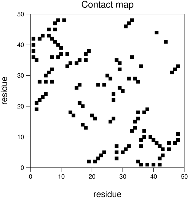
Figure 1: The native conformation used in this study (top) and the corresponding contact map (bottom). Each square in the contact map represents a non-covalent native contact, i.e., a contact that is not a covalent linkage.

Unless otherwise specified, folding is studied at the so-called optimal folding temperature, $T_{opt}$, the temperature that minimizes the folding time, $t$, 21 ; 22 ; 23 ; 24 ; 25 which is computed as the mean first passage time (MFPT) of 100 simulations. This optimal folding temperature may differ from the folding transition temperature, $T_{f}$, at which the probability for finding the protein in an unfolded state is the same as the probability for finding it in the native state. In the context of a lattice model $T_{f}$ may be defined as the temperature at which the average value of the fraction of native contacts $<Q>$ is equal to 0.5 26 . In order to determine $T_{f}$ we averaged $Q$, after collapse to the native state, over MC simulations lasting at least 20 times longer than the folding time computed at $T_{opt}$.

Protein energetics is modeled using the Gō and the Shakhnovich models.

II.2 The Gō model

In the Gō model 27 the energy of a conformation, defined by the set of bead coordinates $\{{\vec{r}}_{i}\}$, is given by the contact Hamiltonian

$$H(\{{\vec{r}}_{i}\})=\sum_{i>j}^{N}\epsilon_{ij}\Delta(\vec{r_{i}}-\vec{r_{j}}),$$ (1)

where the contact function $\Delta({\vec{r}}_{i}-{\vec{r}}_{j})$, is unity if any beads $i$ and $j$ are in contact but not covalently linked, and is zero otherwise. The Gō potential is based on the idea that the native fold is very well optimized energetically. Accordingly, it ascribes equal stabilizing energies, $\epsilon_{ij}=-1.0$, to all pairs of beads $i$ and $j$ that form a contact in the native structure, and neutral energies, $\epsilon_{ij}=0$, to all non-native contacts.

II.3 The Shakhnovich model

By contrast with the Gō model, which ignores the protein’s chemical composition, the Shakhnovich model (see e.g., 28 ) addresses the dependence of protein folding dynamics on the amino acid sequence by considering interactions between the $20$ different amino acids used by Nature in the synthesis of real proteins. Accordingly, the contact Hamiltonian that defines the energy of each conformation is given by

$$H(\{\sigma_{i}\},\{{\vec{r}}_{i}\})=\sum_{i>j}^{N}\epsilon(\sigma_{i},\sigma_{j})\Delta({\vec{r}}_{i}-{\vec{r}}_{j}),$$ (2)

where $\{\sigma_{i}\}$ represents an amino acid sequence, and $\sigma_{i}$ stands for the chemical identity of bead $i$. In this case both the native and the non-native contacts contribute energetically to the folding process. The interaction parameters $\epsilon$ are taken from the $20\times 20$ Miyazawa-Jernigan matrix, derived from the distribution of contacts of native proteins 29 .

Two non-homologous sequences, numbered 1 and 2, were studied within the context of the Shakhnovich model. The latter were designed to fold into the native conformation shown in Figure 1 with the method developed by Shakhnovich and Gutin based on random heteropolymer theory and simulated annealing techniques 30 .

Table 1 summarizes some kinetic and thermodynamic properties of the model proteins discussed above.

Sequence	Enat	Topt	Tf	$\log_{10}({t})$
Gō	$-57.00$	0.65	0.770	5.95 $\pm$ 0.03
$1:$ EPEWQLEFDNSNYAWPANYAQHLPGMYRFTVFDMQRNHTSCKLCFLFS	$-24.34$	0.29	0.305	6.84 $\pm$ 0.04
$2:$ CIFDLEFECPAFPAPIGWLGLVSVVYLFPVRYCRLCMFNCRFKTKTRC	$-26.84$	0.32	0.332	6.53 $\pm$ 0.04

Table 1: Kinetic and thermodynamic properties of the three model proteins. The folding time, $t$, is measured at the optimal folding temperature, $T_{opt}$. Also shown is the folding transition temperature, $T_{f}$, and the native state’s energy $E_{nat}$.

III A general strategy to identify the folding nucleus

We define the FN as a specific set of native contacts which, once formed, prompts rapid and highly probable folding to the native state. In what follows we render a methodology to investigate the existence of folding nuclei in the folding of 48-mer lattice polymers whose energetics are modeled by the Gō or by the MJ potential.

The vast majority of small (i.e. with less than 100 amino acids), single domain proteins fold in a two-state manner with a relaxation rate following single-exponential kinetics 31 . Two-state folding is often rationalized through a ‘classical’ mass-action scheme 32 . Accordingly, the ensemble of conformations that make up the unfolded state ($U$) is separated from the native fold ($N$) by a free energy barrier along some appropriately defined reaction coordinate. The ensemble of conformations that lie on the top of the reaction barrier is the so-called transition state (TS). By definition, TS’s conformations have folding probability $P_{fold}=1/2$ (in other words, TS’s conformations have a probability 0.5 to fold before they unfold) 33 . If folding occurs via nucleation, conformations that rapidly reach the native state with high probability $P_{fold}\gg 1/2$ are post-transition state conformations in which the FN is formed. The latter is indeed a postcritical FN since its formation inevitably leads to the formation native state 4 . In the present study we are therefore interested in postcritical folding nuclei. An appropriate structural analysis of a significantly large ensemble of such conformations should therefore reveal, with a high degree of statistical confidence, a set of common contacts which is the FN. To build such an ensemble we consider 1000 different folding events and, for each individual event, we identify the earliest formed conformation (EFC) that folds rapidly and with high probability, $P_{fold}\geq P^{*}_{fold}$. In order to determine the EFC for a given folding event conformations are sampled at times

$$t_{s}(n)={\rm FPT}-n\Delta t,$$ (3)

where $\Delta t$ is an appropriate sampling interval and $n=1,2,...$. More precisely, starting with $n=1$, the folding probability, $P_{fold}$, of the conformation collected at time $t_{s}(1)$ is computed; this amounts to determining the fraction of folding simulations (in a set of 100 MC runs) which, starting from that conformation reach the native state without passing through conformations with $Q<Q_{U}$, i.e., the protein folds before it unfolds (we consider a protein to be unfolded if its fraction of native contacts is smaller than some cut-off $Q_{U}$). If $P_{fold}<P^{*}_{fold}$ the conformation is discarded. Otherwise, if the folding time $t$ is smaller than some cut-off time $t_{max}$, the procedure described above is repeated for $n=2$ etc. The EFC for a given folding event is the conformation corresponding to the largest $n$ which has $P_{fold}\geq P^{*}_{fold}$ and $t<t_{max}$. In the following section we discuss in some detail the procedure used to fix the parameters $Q_{U}$, $\Delta t$ and $t_{max}$.

III.1 Nucleation in the Gō model

III.1.1 Determination of $Q_{U}$, $t_{max}$ and $\Delta t$

While it is trivial to identify the native state (since is the unique conformation with $Q=1.0$) it is not straightforward to decide weather a conformation belongs to the ensemble of unfolded conformations or is kinetically close (i.e., rapidly converts) to the native state.

The fraction of native contacts $Q$ has been extensively used in simulation studies as a reaction coordinate, i.e., as a parameter that quantifies the degree of folding 26 ; pande ; sali ; socci . In general, however, $Q$ measures closeness to the native structure in energetic (or thermodynamic) terms only. It has been argued that, unless the energy landscape is considerably smooth, thermodynamic closeness does not necessarily imply kinetic proximity to the native structure 34 . However, even if the suitability of $Q$ as a reaction coordinate is questionable, very small $Q$s must necessarily identify unfolded conformations (i.e., that are thermodynamically and kinetically distant from the native fold ).

In order to distinguish unfolded conformations from other conformers we have computed the probability of finding a conformation with a fraction of native contacts $Q$ as a function of $Q$ in a sample of 200 different folding events. Two peaks are apparent in the graph reported in Figure 2: a high-probability peak centered at $Q=0.088$ and another one, of considerably lower probability, that appears immediately prior to the native fold. The high probability peak is clearly associated with the unfolded states. The cut-off $Q_{U}$ is chosen such that more than half of the unfolded peak lies to the left of $Q=Q_{U}$. In what follows we take $Q_{U}=0.15$ but note that other values of $Q_{U}$ were tested and were found to lead to the same results.

The probability for the protein to be in high-$Q$ conformations is small but non negligible (Fig 2). This happens because the optimal folding temperature $T_{opt}$, at which data was collected, is well below the system’s folding transition temperature $T_{f}$ (Table 1). Accordingly, the protein may be trapped in low energy conformations that share a high degree of structural similarity with the native fold (i.e., whose fraction of native contacts is $Q\sim 0.8$).

Figure 2: Probability of finding a conformation with fraction of native contacts $Q$ a function of $Q$. $Q_{U}$ is the fraction of native contacts below which the protein is considered to be unfolded. The probability of $Q=1.0$ vanishes since the simulation stops when the protein reaches the native state.

By definition, the formation of the FN prompts rapid and highly probable folding ($P_{fold}\geq P^{*}_{fold}$). The cut-off parameter $t_{max}$ (i.e., the maximum number of MC steps in which the protein is required to reach the native fold) is therefore a particularly important step of the procedure proposed to identify the FN.

A tentative sampling interval (about 2 orders of magnitude smaller than the folding time for this model protein) was used to collect an ensemble of $\sim 2000$ conformations with $P^{*}_{fold}=1$ from 100 different folding events. The vast majority ($>90$%) of such conformations were found to reach the native state in time $t$ less than $1.4$x$10^{4}$ MCS while about 10% take a considerably longer time to fold (Figure 3).

Two (folding) time scales are clearly distinguished in this ensemble of conformations. The shorter time scale corresponds to conformations where the FN has the highest probability of being formed, while the longer one is associated with folding events during which the protein is trapped in low energy states which, despite despite sharing a large similarity with the native fold, do not have the FN formed (Figure 2). In order to eliminate the latter conformations $t_{max}$ was set to $1.4$x$10^{4}$ MCS.

Figure 3: Fraction of unfolded conformations as a function of time (in a $\log_{10}$-scale). About 90% of the conformations fold in $1.4$x10⁴ MCS while the remaining 10% fold in times that are about one order of magnitude longer.

The efficiency of the sampling procedure may be improved by choosing the sampling interval, $\Delta t$, appropriately. Let $\rm FPT-FPT_{\rm EFC}$ be the number of MC steps required to complete folding once the EFC forms at time $\rm FPT_{\rm EFC}$ in a given folding event. We define $t_{\rm EFC}$ as the average folding time of the EFC of 100 folding events (i.e., $t_{\rm EFC}$ is the average of $\rm FPT-FPT_{\rm EFC}$ computed over 100 folding events). Ideally, the sampling interval should be smaller than $t_{\rm EFC}$, or at least of the same order of magnitude. In practice, for a tentative $\Delta t$, we compute $t_{\rm EFC}$ by averaging $N\Delta t$ in 100 folding events where $N$ is the maximum value of $n$ for each event. We fix $\Delta t$ if the corresponding $t_{\rm EFC}$ lies between 5$\Delta t$ or 10$\Delta t$. For the model protein considered in this section we have found that $t_{\rm EFC}\sim 6000$ for $\Delta t=1000$ MCS, which means that, on average, the EFCs are collected at a sampling time $t_{s}(6)$.

In Figure 4 the dependence of $P_{fold}$ on $n$ is shown for a single folding event. The folding probability is zero when $n=16$ but as time approaches the FPT (i.e. for $n<16$) the protein explores a series of conformations, with $P_{fold}\neq 0$ and reaches the native state with $P_{fold}=1$ when $n=0$. The conformations corresponding to $n=1$ and $n=2$ have $P_{fold}=1$ as well and reach the native state in time $t_{f}<t_{max}$. Thus, the EFC for this folding event is the conformation which corresponds to $n=2$.

Figure 4: A typical plot of $P_{fold}$ as a function of $n$ (with $\Delta t=1000$). Conformations collected at small $n$ have a very high $P_{fold}$ and some of them have $P_{fold}=1$.

III.1.2 A folding nucleus determined solely by native topology

Having fixed the parameters $Q_{U}$, $\Delta t$ and $t_{max}$ we ran 1000 different folding events from which an ensemble of 1000 conformations (one conformation per folding run) were collected. The latter are all EFCs, i.e., the earliest conformations in folding events that collapse rapidly to the native state (i.e., their folding time is $t<t_{max}=14000$ MCS) with unit folding probability. The average fraction of native contacts of this ensemble of conformations is $<Q>_{\rm EFC}=0.67$.

We start by labeling the 57 native contacts as in Table 2.

Contact	Ri :	Rj	Contact	Ri :	Rj	Contact	Ri :	Rj	Contact	Ri :	Rj	Contact	Ri :	Rj
0	0 :	41	12	6 :	35	24	21 :	26	35	32 :	35	46	5 :	44
1	7 :	44	13	23 :	26	25	5 :	42	36	1 :	20	47	14 :	33
2	10 :	47	14	27 :	34	26	6 :	41	37	2 :	21	48	15 :	34
3	11 :	32	15	28 :	33	27	7 :	40	38	3 :	22	49	17 :	36
4	12 :	33	16	0 :	35	28	8 :	39	39	4 :	23	50	18 :	37
5	14 :	25	17	1 :	34	29	9 :	38	40	6 :	27	51	24 :	29
6	15 :	26	18	2 :	27	30	11 :	36	41	8 :	35	52	25 :	28
7	17 :	34	19	4 :	29	31	12 :	17	42	9 :	36	53	28 :	31
8	40 :	43	20	5 :	30	32	13 :	16	43	0 :	39	54	30 :	45
9	0 :	37	21	6 :	31	33	15 :	20	44	2 :	41	55	31 :	46
10	1 :	18	22	7 :	46	34	16 :	19	45	3 :	42	56	32 :	47
11	4 :	27	23	8 :	47

Table 2: For structures that like ours are maximally compact cuboids with $N=48$ residues there are 57 native contacts. This table displays the correspondence between the contact number and the pair of residues involved in each contact.

For each native contact we define the contact probability as the number of conformations in which the contact is formed normalized to the total number of conformations in the sample. Results reported in Figure 5 show that the contact probability varies considerably among the 57 native contacts, an observation that is particularly evident for probabilities larger than 50%. This finding strongly suggests that, while the establishment of some contacts (e.g., 12 and 41, which are present in over 95% of the conformations analyzed) is an essential requirement to ensure rapid folding, the formation of others (e.g., 2 and 54 which appear with probability $<$40%) does not appear to be a requisite to fast folding. The set of 9 contacts, involving residues 6, 8, 9, 11, 28, 31-33, 35, and 36 (Figure 6, left), and identified by contact number in Figure 5, seems to be particularly relevant. Indeed, each individual contact is formed in more than 85% of the conformations analyzed, and all of the 9 contacts are simultaneously formed in 64% of the conformers. Moreover, on average, $8.2$ of them are present in the ensemble of conformations considered.

The fact that rapid folding is associated with the formation of a set of highly probable contacts suggests that such a contact set is the FN.

There is, of course, a certain degree of arbitrariness in the choice of the probability cut-off that is used to identify the highly probable contacts, and therefore the set of contacts identified above is a putative FN.

Figure 5: The contact histogram for the Gō model showing, for each native contact, the probability of being formed in the ensemble of 1000 EFC conformations that fold in time $t<1300$ MCS with unit folding probability. The nine contacts identified by number have the highest probability (i.e. probability $>85$%) of being formed.

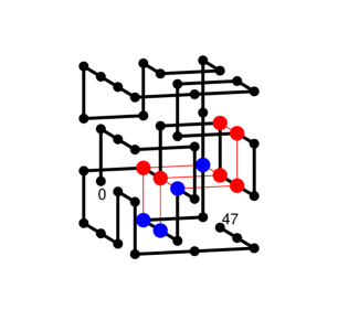
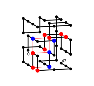
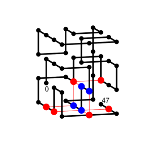
Figure 6: The folding nucleus for the Gō model (left), for sequence 1 (center) and for sequence 2 (right) is the set of 9, 10 and 8 contacts, respectively, colored in red. Residues whose number along the sequence is less than 12 are colored in blue and those whose number along the sequence is larger than 26 are colored in red.

III.2 Nucleation in the Shakhnovich model

In order to investigate the importance of amino acid sequence in the formation of the FN, we studied the folding of two non-homologous sequences (numbered 1 and 2) (Table 1).

III.2.1 Determination of $Q_{U}$, $\Delta t$ and $t_{max}$

In the Gō model the so-called topological frustration 36 results from polymer properties of the chain such as connectivity 9 ; 33 , excluded volume effects, and quirks of the native topology, such as lack of symmetry 37 . Topological frustration is the only type of frustration in models which, like the Gō model, are native centric. On the other hand, by taking into account the protein chemistry, the Shakhnovich model also exhibits energetic frustration. The latter typically leads to longer folding times and, at temperatures below the folding transition temperature, the chain is prone to get trapped in low energy states 37 . This implies that, in contrast with the Gō model, for which $T_{opt}$ is well below $T_{f}$, the two Shakhnovich protein sequences have optimal folding temperatures which are close to the system’s folding transition temperatures (Table 1). Thus, although the observed folding times are longer than those found for the Gō model (Table 1), the Shakhnovich model proteins do not get trapped in high-$Q$, low energy states. Indeed, the $Q$ probability distributions are not peaked in the high-$Q$ ($Q\sim 0.8$) region (Figure 7) although both models exhibit a well defined, high-probability low-$Q$ peak, at $Q=0.20$, corresponding to the unfolded states. Applying the same criterion for the choice of cut-off $Q_{U}$, one considers a conformation unfolded if $Q<Q_{U}=0.25$. As before, we have found that the results for the FN are robust with respect to small variations in the choice of $Q_{U}$.

Figure 7: Probability of having a conformation with fraction of native contacts $Q$ for sequences 1 (top) and 2 (bottom). The peak at small $Q$ is well defined for both model proteins. The probability curve for sequence 2 falls sharply to zero as $Q$ increases, while for sequence 1 there is a small probability for the system to be found in conformations with $0.5<Q<0.7$. In either case the protein is considered to be unfolded when the fraction of native contacts is smaller than $Q_{U}=0.25$.

In order to fix $t_{max}$, a set of $\sim$ 1200 conformations (per sequence), with $P^{*}_{fold}=0.90$, is collected from 100 different folding events and the corresponding folding times are measured. For sequence 1, two folding time scales are observed (Figure 8, top). The fraction of native contacts in the ensemble of sequence 1’s conformations is $Q=0.72\pm 0.12$. Since there is a small probability for sequence 1 to be in conformations with $Q\sim$ 0.7 (Figure 7) the longer time-scale may be ascribed to the population of these relatively high-$Q$ conformations which, being local energy minima, will slow down folding. In order to disregard these conformations the cut-off time is set to $t_{max}=30000$ MCS. By contrast, for sequence 2 the folding times are all of the same order of magnitude (Figure 8, bottom) and there is no need to use a cut-off time, $t_{max}$.

The reason for taking $P^{*}_{fold}=0.9$, instead of $P^{*}_{fold}=1.0$ as in the Go model, is that the latter leads, in the Shakhnovich model, to an ensemble of conformations with a high average fraction of native contacts ($<Q>\sim 0.85$). The latter are practically folded and thus are not suitable to distinguish the contacts that belong to the FN from other trivial contacts.

Figure 8: Fraction of unfolded conformations as a function of time starting from conformations with $P_{fold}>0.90$. For sequence 1 (top) two time-scales, differing by one order of magnitude, may be observed. In order to select the fastest folders the cut-off time is fixed at $t_{max}=30000$ MCS. For sequence 2 (bottom) there is no need to use a cut-off time since all folding are of the same order of magnitude.

To improve the efficiency of the sampling procedure we have, also for the Shakhnovich model proteins, optimized the sampling intervals as described previously. We have found that $\Delta t=1000$ MCS works well for both proteins yielding $t_{\rm EFC}\sim 9500$ MCS and $t_{\rm EFC}\sim 14000$ MCS for sequence 1 and 2 respectively, i.e., on average the EFCs for sequence 1 are collected at $t_{s}(10)$ while for sequence 2 they are collected at $t_{s}(14)$.

III.2.2 Folding nuclei determined by topology and protein sequence

Two ensembles, each comprising 1000 EFCs, were obtained for sequences 1 and 2 using the parameters discussed in the previous section, with $<Q>_{EFC}=0.65$ and $<Q>_{EFC}=0.62$ for sequences 1 and 2 respectively. These values of $<Q>$ are similar to that of the Gō model and considerably lower than those obtained if $P^{*}_{fold}=1.0$ is used for the Shakhnovich model, allowing the distinction of the contacts in a putative FN from other spurious contacts.

The native structure of sequences 1 and 2 is the same as that of the Gō model and the same numbering of native contacts is used (Table 2).

Figure 9: Contact histograms for sequence 1 (top) and sequence 2 (bottom). Contacts present with the highest probability ($>95\%$) are identified by contact number.

From the analysis of the contact histograms we observe that some native contacts are present with very high probability ($>95\%$)(Figure 9). We consider the putative FN as the set of the most probable contacts.

For sequence 1 the FN is thus formed by 10 native linkages (identified by contact number in Figure 9, top) involving 12 residues (namely, 2, 4, 6, 7, 27, 28, 33, 34, 35, 40, 41, and 43)(Figure 6, center). The 10 contacts forming the FN are simultaneously present in 82% of the EFC conformations analyzed and, on average, the latter have 9.7 of these contacts formed. It is interesting to note that the average stability of the contacts forming the FN is 62% higher than the average stability of the 57 native contacts of the folded protein (Table 3). For sequence 2 the FN is formed by 8 native contacts (identified by contact number in Figure 9, bottom) and 10 residues (namely, residues 5, 6, 7, 8, 32, 35, 39, 40, 44, and 46) (Figure 6, right). The 8 contacts forming the FN are simultaneously present in 90% of the EFC conformations analyzed and, on average, the latter have 7.9 of these contacts formed. In this case the average stability of the FN’s contacts is 53% higher than the average stability of the protein’s native contacts (Table 3).

The two folding nuclei have 2 native contacts (12 and 27) and 4 residues in common. These native contacts are non-local linkages between residues 6 and 35 and between residues 7 and 40, suggesting that the establishment of the corresponding long range interactions might be determinant to ensure rapid folding.

Structurally speaking the FN of sequence 1 consists of two loops, one formed by residues 2, 27, 41, and 6 and the other by residues, 41, 6, 40, and 7 (Figure 6, center). Each of these loops is formed by contacts located in the interior of the protein, while in sequence 2 a significant fraction of the FN’s contacts are located on the fold’s surface (Figure 6, right).

III.3 Nucleation scenarios and contact stability

The Gō FN shares 22% of its contacts with sequence 1 and 33% with sequence 2. The presence of these contacts in the folding nuclei of the Shakhnovich models is driven by native topology. Indeed, the average stability of the Shakhnovich contacts that are also present in the Gō model is up to 25% lower than the average stability of the remaining contacts in the FN (Table 3, columns 3 and 4) but they are formed with equally high probability $>95$%.

The extremely high probability ($\sim$1) of the contact between residues 6 and 35 (i.e. contact 12 in the contact histograms) in all the three model proteins is a robust feature of the nucleation mechanism. Another interesting observation regarding these residues is that they make-up a network of 7 native contacts in the fold (whose average range is 25 units of backbone distance) and about half of these contacts are present in each FN which suggests that they might be key residues in the folding process. We have performed exhaustive single-point mutations in all of the 48 residues and, in agreement with the above hypothesis, we have found that two mutations, one on residue 6, and the other on residue 35, lead to the largest increases in folding times (the folding time increases by up to 6-fold with respect to that of the wild-type sequence) 38 .

The average stability of the Gō FN’s contacts that do not participate in the Shakhnovich folding nuclei, of sequences 1 and 2, is up to 66% lower than the protein’s 57 native contacts (Table 3, columns 1 and 5). By contrast, the contacts that are exclusive to the Shakhnovich folding nuclei are up to 90% more stable than the protein’s 57 native contacts (Table 3, columns 1 and 4). Moreover, as we have already pointed out, the Shakhnovich folding nuclei are up to 81% more stable than the protein’s 57 native contacts (Table 3, columns 1 and 2).

Clearly, by ascribing different stabilities to the protein’s native contacts, the protein sequence promotes an overall change of the nucleation scenario, which in the Gō model is driven solely by the topological features of the native fold. To see how this happens in more detail we investigated the effect of contact stability in the contact histogram (i.e. in the determination of the FN) of sequence 2. The most stable contacts in this case are contacts 1, 16, 23, 25, 28, 35, 41, 43, 46, 56 (Figure 10) and, not surprisingly, half of them belong to the FN (Figure 9). It is interesting to note that, by being particularly stable, some contacts may indirectly promote an increase in the probability of occurrence of other less stable contacts. This feature is well illustrated by residue 47 and the three contacts it establishes in the fold. The latter appear with considerably high probabilities in the contact histogram. The probabilities of contacts 23 and 56 (which are considerably lower in the Gō model) may be ascribed to their very high stabilities. However, contact 2 is a neutral one and, in spite of its relative low stability, its probability is higher when compared with other stable contacts in the protein. This presumably happens because the very high stability of contacts 23 and 56 forces residue 47 to be in its native environment (i.e. to have all of its native contacts formed simultaneously) which naturally increases the probability with which contact 2 is formed.

Stability is indeed a considerably determinant factor for the Shakhnovich FN, but is not the whole story. The presence of Gō contacts in the nucleus, is not energetically favorable (Table 3, columns 2 and 3), but is very relevant from a functional point of view as discussed in the next section.

Mean energy per contact
	protein	SFN	SFN $\wedge$ GōFN	SFN $\wedge$ ($\sim$ GōFN)	($\sim$ SFN) $\wedge$ GōFN
Sequence 1	-0.427	-0.691	-0.579	-0.719	-0.424
Sequence 2	-0.471	-0.854	-0.783	-0.896	-0.283

Table 3: Mean energy per contact in different contact sets. In the the first column the average is computed over the protein’s 57 native contacts. S_FN stands for the Shakhnovich FN and Gō_FN stands for the Gō FN. Accordingly, the second column displays the contact’s mean energy in S_FN; the contact’s mean energy in the set of contacts that are common to the Shakhnovich nuclei and Gō_FN is shown in the third column. The fourth column refers to the set of contacts that are in S_FN but not in Gō_FN and finally, in the fifth column, one considers the contacts that are in Gō_FN but not in S_FN.

Figure 10: Energy of each native contact. Half of the most stable contacts, identified in the figure by contact number, are present in sequence’s 2 folding nucleus.

III.4 The ‘topological’ role of the folding nucleus

Despite clear differences, which are driven by contact stability, the three folding nuclei are nonetheless topologically similar. The residues that participate in the set of native contacts forming the folding nuclei split into two groups located in different regions of the protein chain. Indeed, in all cases there is a group of 4 residues located in one region of the chain that comprises residues 2 to 11 and there is another group of 6 (or 8) residues located in a distant part of the chain that extends between residue 27 and residue 46. This is illustrated in Figure 6 where the residues whose number along the sequence is less than 12 are colored in blue while those whose number along the sequence is larger than 26 are colored in red. It then follows that more than two thirds of the contacts that make up the folding nuclei are non-local contacts whose range lies between 18 to 30 units of backbone separation. In the three protein models the FN performs the same ‘topological’ role, that of linking residues located in two distant parts of the protein chain.

IV Conclusions

In the present work we have proposed and discussed in detail a methodology to the identify the folding nucleus (i.e. a specific subset of native contacts which, once formed, prompts very rapid and highly probable folding) in small lattice proteins and applied it to investigate the nucleation mechanism of three model proteins with chain length N=48. We have found that a folding nucleus (FN) which is solely driven by the native fold’s topological features (as it happens in the Gō model) is not globally robust with regard to protein sequence. The latter distinguishes native contacts, based on the stability of their interaction energies, and the nucleation pattern is biased towards the most stable contacts. In other words: in a (more realistic) lattice model, like a sequence-specific one, the FN is, to some extent, formed by the most stable contacts, and the presence of other less stable contacts in the FN is uniquely determined by the fold’s topology. However, we have found that, independently of protein sequence, the residues forming the three folding nuclei are distributed along the protein chain in a similar and well defined manner. Accordingly, the nucleation mechanism comprises the coalescence of two distinct and distant parts of the protein chain through the establishment of the long range interactions corresponding to the non-local contacts forming the FN. Therefore we conclude that the fold’s topology determines, to a large extent, the overall position of the FN in the protein chain. However, as shown by Tiana et al. tiana , sequences as dissimilar as ours may have a different set of key residues (e.g. residues 6 and 35 in our models) in the FN, which may lead to the latter being topologically distinct.

A particularly interesting finding of this work regards the existence of 2 residues which, in the three model systems, are involved in about 30% of the contacts forming the FN and appear to be determinant in ensuring fast folding. We speculate that the network of native contacts formed by these residues is sufficient to determine the overall fold of the protein in a way that is similar to that found by Vendruscolo et al. 40 for a 98-residue protein model off-lattice.

Previous simulation efforts on lattice models have focused on smaller (namely N=28 5 and N=36 4 ) as well as on proteins with the same chain length 39 . We have found that the size of the FN is similar to the size of the nuclei identified by Shakhnovich and collaborators (containing between 8 and 11 native contacts) which suggests that, at least for small proteins, the size of the FN does not depend on the size of the chain. This could provide an explanation for the small correlation between chain length and folding rates found in real proteins 41 ; gal ; pra .

Generalizations of the methodology described here, may be useful to investigate the folding pathways of model proteins. A very preliminary analysis of our data indicates that there is a higher degree of structural similarity among the EFCs of the Shakhnovich model than among those of the Gō model. Indeed, we have determined how many different native contacts exist between each pair of conformations in the three ensembles that were used to identify the FNs (i.e. in the three ensembles of EFCs) and computed its mean value over the total number of possible pairs. We have found that, on average, two EFCs in the Gō model differ by 11.3 native contacts. Sequences 1 and 2, on the other hand, differ by 9.7 and 7.2 native contacts respectively. We speculate that the higher structural similarity between conformations in the Shakhnovich model may be related to a smaller number of rapid folding pathways. However, a definite conclusion requires further quantitative analysis.

V Acknowledgements

PFNF would like to thank Fundação para a Ciência e Tecnologia (FCT) for financial support through grant SFRH/BPD/21492/2005. This work was also supported by FCT’s grants POCI/FIS/55592/2004 and POCTI/ISFL/2/618. RDMT wishes to thank Eugene Shakhnovich and Guido Tiana for helpful and elucidating discussions.

References

- (1) Kim PS, Baldwin RL 1982 Annu. Rev. Biochem. 51 459
- (2) Baldwin RL, Rose GD 1999 TIBS 24 77
- (3) Karplus M, Weaver DL 1979 Biopolymers 18 1421
- (4) Abkevich VI, Gutin AM and Shakhnovich EI 1994 Biochemistry 33 10026
- (5) Lewyn L, Mirny LA, Shakhnovich EI 2000 Nature Struct. Biol. 7 336 200
- (6) Fersht AR Proc. Natl. Acad. Sci. USA 92 10869
- (7) Wetlaufer DE 1973 Proc. Natl. Acad. Sci. USA 70 697
- (8) Klimov DK, Thirumalai D 1998 J. Mol. Biol. 282 471
- (9) Makarov DE, Plaxco KW 2003 Prot. Sci. 12 17
- (10) Broglia, RA and Tiana G 2001 J. Chem. Phys. 114 7267
- (11) Tiana G, Broglia RA, 2001 J. Chem. Phys. 114 2503
- (12) Wallin S, Chan HS 2005 Protein Sci. 14 1643
- (13) Wallin S, Chan HS 2006 J. Phys. Condens. Matt. 18 307
- (14) Plaxco KW, Simmons KT, Baker, D 1998 J. Mol. Biol. 277 985
- (15) Gromiha MM, Selvaraj S 2001 J. Mol. Biol. 310 27
- (16) Zhou H, Zhou Y 2002 Biophys. J. 82 458
- (17) Micheletti C 2003 Proteins Struct. Funct. Genet. 51 74
- (18) Mirny L, Shakhnovich EI 2001 Ann. Rev. Biomol. Struct. 30 361
- (19) Galzitskaya OV 2002 Molecular Biology 36 386
- (20) Shakhnovich EI 2006 Chem. Rev. 106 1559
- (21) Metropolis N, Rosenbluth AW, Rosenbluth MN, Teller AH, Teller, E 1953 J. Chem. Phys. 21 1087
- (22) Landau DP, Binder KA 2000 A Guide to Monte Carlo Simulations in Statistical Physics. pp. 122-123, Cambridge University Press.
- (23) Gutin AM, Abkevich, VI, Shakhnovich, EI 1996 Phys. Rev. Lett. 77 5433
- (24) Gutin AM, Abkevich VI, Shakhnovich EI 1998 Fold. Desg. 3 183
- (25) Cieplack M, Hoang TX, Li MS 1999 Phys. Rev. Lett. 83 1684
- (26) Faisca PFN Ball, RC 2002 J. Chem. Phys. 116 7231
- (27) Faisca PFN, da Gama MM, Nunes, A 2005 Prot. Struc. Func. Bio. 60 712
- (28) Abkevich VI, Gutin AM, Shakhnovich EI 1995 J. Mol. Biol. 252 460
- (29) Go N, Taketomi H 1978 Proc. Natl. Acad. Sci. USA 75 559
- (30) Shakhnovich EI 1994 Phys. Rev. Lett. 72 3907
- (31) Miyazawa S, Jernigan RL 1985 Macromolecules 18 534
- (32) Shakhnovich EI, Gutin AM 1993 Proc. Natl. Acad. Sci. USA 90 7195
- (33) Jackson SE 1998 Fold Des. 3 81
- (34) Dill KA 1999 Protein Sci. 8 1166
- (35) Du R, Pande VS, Grosberg AYu, Tanaka T, Shakhnovich EI 1998 J. Chem. Phys. 111 10375
- (36) Pande VS, Grosberg AYu, Tanaka T 1997 Fold. Desg. 2 109
- (37) Sali A, Shakhnovich EI, Karplus M 1994 Nature 369 248
- (38) Socci ND, Onchic JN, Wolynes PG 1996 J. Chem. Phys. 104 5860
- (39) Chan HS, Dill KA 1998 Prot. Struc. Func. Gen. 30 2
- (40) Nelson ED, Teneyck LF, Onuchic JN 1997 Phys. Rev. Lett. 79 3534
- (41) Gutin A, Sali A, Abkevich V, Karplus M, Shakhnovich EI 1998 J. Chem. Phys. 108 6466
- (42) Faisca PFN, da Gama MMT, Ball RC, Shakhnovich EI 2006, in preparation
- (43) Tiana G, Broglia RA, Shakhnovich EI 2000 Prot Struc. Func. Gen 39 244
- (44) Vendruscolo M, Paci E, Dobson CM, Karplus M 2001 Nature 409 641
- (45) Shakhnovich E, Abkevich V, Ptitsyn O 1996 Nature 379 95
- (46) Plaxco KW, Simmons KT, Ruczinski I, Baker D 2000 Biochemistry 39 11177
- (47) Galzitskaya OV, Grabuzynskiy SO, Ivankov DN, Finkelstein AV, Protein Sci 2003 51 162
- (48) Prakash N, Bhuyan AK Biochemistry 2006 45 3805