Back-stepping, hidden substeps, and conditional dwell times in molecular motors

Abstract

Processive molecular motors take more-or-less uniformly sized steps, along spatially periodic tracks, mostly forwards but increasingly backwards under loads. Experimentally, the major steps can be resolved clearly within the noise but one knows biochemically that one or more mechanochemical substeps remain hidden in each enzymatic cycle. In order to properly interpret experimental data for back/forward step ratios, mean conditional step-to-step dwell times, etc., a first-passage analysis has been developed that takes account of hidden substeps in $N$-state sequential models. The explicit, general results differ significantly from previous treatments that identify the observed steps with complete mechanochemical cycles; e.g., the mean dwell times $\tau_{+}$ and $\tau_{-}$ prior to forward and back steps, respectively, are normally unequal although the dwell times $\tau_{++}$ and $\tau_{--}$ between successive forward and back steps are equal. Illustrative ($N=2$)-state examples display a wide range of behavior. The formulation extends to the case of two or more detectable transitions in a multistate cycle with hidden substeps.

I Introduction

Processive motor proteins or molecular motors howard ; bray (such as kinesin, cytoplasmic dynein, and myosin V) “walk” along molecular tracks (microtubules and actin filaments) taking observed mechanical steps of well defined (mean) spacing $d$ , each step being of “negligibly short” ($\lesssim 100\,\mu s$) duration relative to the mean time(s) between steps that are of order $1$ to $20\,\textrm{ms}$  howard ; bray ; mehta99 ; rief00 ; nishiyama02 ; block03 ; nishiyama03 ; yildiz03 ; snyder04 ; uemura04 ; baker04 ; oiwa05 ; carter05 ; taniguchi05 ; clemen05 ; guydosh06 ; toba06 . Steps may be taken forwards ($+$) or backwards ($-$). The mean velocity (observed over 10’s to 100’s ) of steps, $V$, is a function of the load $\textbf{F}=(F_{x},F_{y},F_{z})$ exerted on the motor and the fuel concentration [ATP] (for most cases) fisher99 ; kolomeisky03 ; fisher05 and, in general, of other features of the aqueous solution including the pH, ionic strength, temperature $T$, and other reagents/reactants such as [ADP], [Pi], [AMP-PNP], [BeF₂], etc.)howard ; block03 ; carter05 ; guydosh06 .

Motor proteins are enzymatic catalysts that, following biochemical knowledge and principles, turn over one “fuel molecule” (usually ATP) for each full step via (in the simplest case) a linear sequence of reversible kinetic transitions (or reactions) embodying $N$ (bio)chemical states per turnover fisher99 ; kolomeisky03 ; fisher05 ; fisher99a ; kolomeisky00 ; kim05 ; bustamante01 . This situation is embodied in the following basic sequential model

$$\cdots\begin{array}[]{c}u_{N-1}\\ \xleftarrow{\quad\quad\quad}\\ \vspace{-10 mm}\hfil\\ \xrightarrow{\quad\quad\quad}\\ w_{0\equiv N}\end{array}[0]_{l}\begin{array}[]{c}u_{0}\\ \xleftarrow{\quad\quad\quad}\\ \vspace{-10 mm}\hfil\\ \xrightarrow{\quad\quad\quad}\\ w_{1}\end{array}(1)_{l}\begin{array}[]{c}u_{1}\\ \xleftarrow{\quad\quad\quad}\\ \vspace{-10 mm}\hfil\\ \xrightarrow{\quad\quad\quad}\\ w_{2}\end{array}(2)_{l}\begin{array}[]{c}u_{2}\\ \xleftarrow{\quad\quad\quad}\\ \vspace{-10 mm}\hfil\\ \xrightarrow{\quad\quad\quad}\\ w_{3}\end{array}\cdots$$ (21)

$$\cdots\begin{array}[]{c}u_{N-2}\\ \xleftarrow{\quad\quad\quad}\\ \vspace{-10 mm}\hfil\\ \xrightarrow{\quad\quad\quad}\\ w_{N-1}\end{array}(N-1)_{l}\begin{array}[]{c}u_{N-1}\\ \xleftarrow{\quad\quad\quad}\\ \vspace{-10 mm}\hfil\\ \xrightarrow{\quad\quad\quad}\\ w_{N}\end{array}[N]_{l}\equiv[0]_{l+1}\begin{array}[]{c}u_{0}\\ \xleftarrow{\quad\quad}\\ \vspace{-10 mm}\hfil\\ \xrightarrow{\quad\quad}\\ w_{1}\end{array}\cdots,$$ (37)

which is understood to repeat periodically as the motor moves processively along its track. The subscript $l=1,2,\cdots$ labeling the $N$ basic states $[0]$, $(1)$, $\cdots(N-1)$, denotes the sites on the linear track spaced at distance $d$ apart.

By convention the state $(i)=[0]$ is “bound” or “nucleotide-free” so that the transition $[0]\rightarrow(1)$ represents the binding of one fuel molecule to the awaiting motor. Thus we write

$$u_{0}=k_{0}[\mbox{ATP}],$$ (38)

where the pseudo-first-order rate constant $k_{0}$ and all the remaining rate constants $u_{i}$, $w_{j}$ depend also on F. But under fixed conditions (F, [ATP], $\cdots$), the rates do not change. Note that this formulation embodies the tight coupling principle of one fuel molecule being consumed per (forward) step howard ; fisher99 ; kolomeisky03 ; bustamante01 . This is assumed in the basic model, which also neglects irreversible detachments from the track (which, however, can be included readily in principle fisher99 ; fisher99a ; kolomeisky00 ).

When convenient we will allow the state labels $i$, $j$, $\cdots$ to take values outside the basic range $[0,N-1]$; for that reason we adopt the periodicity convention

$$u_{i+lN}\equiv u_{i},\;\;w_{j+lN}\equiv w_{j},\;\;l=0,\pm 1,\pm 2,\cdots.$$ (39)

Now, in the simplest experimental situation, as observed for kinesin, no mechanical substeps are detected nishiyama02 ; carter05 to within the noise level (which amounts to $\Delta x\lesssim 1\,\textrm{nm}$). Furthermore to within the resolution time ($\lesssim 100\,\mu s$), successive steps occur at times, say, $\cdots,t_{k-1},\;t_{k},\;t_{k+1},\cdots$. Thus, between the identifiable mechanical steps of (mean) magnitude $d$, the motor dwells in a mechanical state that, within the noise level $\Delta x$, appears well defined with no systematically detectable substeps, forwards or backwards. Then, individual dwell times in the mechanical states, namely,

$$\tau_{k}=t_{k}-t_{k-1},$$ (40)

can be measured to reasonable precision and averages may be computed, over “many” observations encompassing, say, $n$ steps, to yield an overall mean dwell time

$$\tau=\left<\tau_{k}\right>\approx\frac{1}{n}\sum_{k=1}^{n}\tau_{k}.$$ (41)

Here and below we use the “asymptotically equals” symbol $\approx$ to indicate an approximate equality that becomes exact in a long run under steady-state conditions.

Given a (sufficiently long) sequence of $n$ observed steps with $n_{+}$ forward steps and $n_{-}$ backward steps, we can also define the (steady-state) step splitting probabilities or back-step and forward-step fractions

$$\pi_{+}\approx n_{+}/n,\qquad\pi_{-}\approx n_{-}/n,$$ (42)

where, since $n=n_{+}+n_{-}$, one has

$$\pi_{+}+\pi_{-}=1.$$ (43)

Furthermore, dwell times before a $+$ or $-$ step can be (and have been carter05 ) measured separately leading to distinct prior dwell times

$$\tau_{+}=\frac{1}{n_{+}}\mbox{$\sum^{+}$}\tau_{k}\qquad\mbox{and}\qquad\tau_{-}=\frac{1}{n_{-}}\mbox{$\sum^{-}$}\tau_{k},$$ (44)

the restricted sums including just $+$ or $-$ steps, respectively.

To the degree that the runs are long so that $\pi_{+}$ and $\pi_{-}$ may be accurately considered as probabilities one must evidently also have

$$\pi_{+}\tau_{+}+\pi_{-}\tau_{-}=\tau.$$ (45)

As discussed recently in some detail fisher05 ; kim05 , each individual biochemical state $(i)$, may be characterized by a definite (mean) longitudinal location in physical space, i.e., along the track, which we supposed aligned with the $x$ coordinate, and, possibly, transverse to the track, the $y$-coordinate, or normal to the track, the $z$-coordinate. Hence the basic model implies the existence of substeps, say, of magnitude

$$d_{j}=x_{j+1}-x_{j},$$ (46)

between successive mechanochemical states foot0 . However, the great majority of these mechanical displacements will be hidden by noise and so unobservable. This is the crucial issue.

The evidence (in particular for kinesin nishiyama02 ; carter05 ) reveals the existence of one principal or major mechanical substep of magnitude

$$d_{M}=x_{M+1}-x_{M}\simeq d,$$ (47)

that corresponds to a specific transition $(M)\!\!\rightarrow\!\!(M+1)$ for a forward or $+$ step. Such a unique forward-step is sometimes called a “power stroke”. Then, clearly, within the basic model a back-step ($-$) corresponds to the specific transition $(M+1)\!\rightarrow\!(M)$.

For simplicity we will initially suppose that there is only one such single, well defined and observable principal mechanical transition in the processive reaction cycle: it will be referred to as a major transition while all other smaller, unobservable displacements, presumed “hidden,” will be termed substeps.

It is of interest, all the same, to analyze situations in which, within the full cycle, there are a number of visible (or observable) substeps. Indeed, an initial substep large enough to be readily observable was predicted for myosin V by Kolomeisky and Fisher kolomeisky03 on the basis of dwell-time data obtained at different [ATP] and force levels mehta99 ; it was later observed unambiguously by Uemura et al uemura04 . Thus, in Sec. V below, the case of $K$ ($<N$) distinct major substeps is considered explicitly foot0A .

Nevertheless, since most of the forward and reverse transitions, $(i)\rightarrow(i-1)$ and $(i-1)\rightarrow(i)$, are not observable, one does not know (and cannot tell) the (bio)chemical (sub)state of the motor during an observed dwell time, $\tau_{k}$, between steps $k-1$ and $k$: see (40). Indeed, the biochemical state will change as time progresses and not necessarily in a uniform sense, e.g., ATP might bind and then be released (or unbind) without undergoing a hydrolysis step. For this crucial reason once the basic model has $N=2$ or more states the expressions for $\tau_{+}$ and $\tau_{-}$ in terms of the basic rates $u_{i}$ and $w_{j}$ cannot be trivial — and the same goes for the splitting or backwards and forwards probabilities $\pi_{+}$ and $\pi_{-}$.

The basic theoretical problem is thus to find explicit expressions for $\pi_{+}$, $\pi_{-}$, and for the partial dwell times as well as for conditional or pairwise stepping fractions, $\pi_{++}$, $\pi_{-+}$, $\cdots$, and dwell times, $\tau_{++}$, $\tau_{-+}$, $\cdots$, that it is natural to introduce (as seen below). Indeed, it is clear that these general statistical concepts are not restricted to linear or translocational motors, on which we have focussed; in fact, they apply equally to rotary stepping motors like F₁-ATPase yasuda98 ; shimabukuro03 ; nishizaka04 ; shimabukuro05 , F₁F₀-ATPase diez04 ; ueno05 , and bacterial flagellar motors bray ; sowa05 . However, since, in these respects, kinesin and myosin V have been studied more extensively, we will retain the language appropriate for processive motor proteins walking on linear tracks.

In previous theoretical studies kolomeisky03 ; kolomeisky05 ; qian06 ; wang06 splitting probabilities and conditional mean dwell times have been introduced in the context of molecular motors via the following definitions (which are distinguished from those used in the discussion above by haceks) specifically: $\check{\pi}_{+}\equiv\pi_{0,N}$ and $\check{\pi}_{-}\equiv\pi_{0,-N}$ are the probabilities that a motor starting at a well defined physical site $l$ along the track in the binding state $(j)=[0]$ will arrive at the next site $l+1$ or back at the previous site $l-1$ (in both cases in state $(j)=[0]$) without having undergone the opposite transition to complete a full backward or forward cycle, respectively. Then, similarly, $\check{\tau}_{\pm}\equiv\tau_{0,\pm N}$ are the average times a motor spends at site $l$ (starting at $j=0$) before completing a full forward or backward cycle to site $l\pm 1$ (in state $(j)=[0]$). Exact results for such statistics can be derived by mapping into a Markov renewal process qian06 ; wang06 .

With these definitions the explicit formulae obtained kolomeisky03 ; kolomeisky05 for $\;\check{\pi}_{\pm}\;$ and $\;\check{\tau}_{\pm}\;$ correspond to a full mechanochemical cycle during which a complete forward or backward step is certainly taken. However, the resulting expressions can be applied to the analysis of experimental stepping data only if these data allow one to identify each full cycle. If, instead, the observed noise hides one or more of the $N>1$ biochemical or mechanochemical substeps, while only major mechanical transitions are detectible, one cannot in general decide unambiguously whether a motor executed the detectable steps (or power strokes) with or without completing a full cycle. In such cases, the previous expressions cannot be applied to account for the observed step fractions and dwell times $\pi_{\pm}$ and $\tau_{\pm}$. Instead, the results must be modified to allow for the ambiguity arising from the hidden substeps. It transpires, as we show below, that this rather subtle and at first-sight inconsequential small difference actually leads to significant changes in the load dependence especially (but not exclusively) when the fractions of back-steps and forward-steps are similar in frequency, i.e., on approaching stall conditions when the velocity, $V$, becomes small relative to its load-free value fisher99 ; kolomeisky03 ; fisher05 .

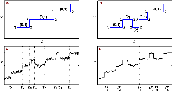
Figure 1: Schematic graphs illustrating why the full-cycle interpretation is not adequate for describing stepping data: Plot (a) depicts a hypothetical time series of forward steps for an ($N=4$) cycle with $M=2$. The (0,1)’s indicate that the states $[0]_{l}$ and $(1)_{l}$ are both certain to occur at least once between the pairs of states $(3)_{l-1}$ and $(2)_{l}$. (See the text.) Then (b) represents a similar time series but with one major back-step. The question-marks between the forward-back and back-forward steps indicate that one does not know if the motor has ever passed through the states $[0]_{l}$ and/or $(1)_{l}$ in these intervals. Finally, (c) and (d) depict two equivalent time series for a motor with $N=3$ and $M=1$ but with different noise levels. The first plot allows one to identify only major forward and backward transitions at times $t_{k}$ (marked on the axis) while the states $[0]_{l}$ and corresponding substeps are hidden in the noise. However, the second plot reveals all the transitions and substeps, so that the $t^{0}_{k}$, marking the beginning (or end) of each full cycle, can be determined. These schematic examples demonstrate that detectable transitions do not necessarily correspond to a full biochemical cycle so that a proper statistical analysis must take account of substeps hidden in the noise. Notice, indeed, that the three major transitions identified as forward and back steps at times $t_{3}$, $t_{4}$ and $t_{5}$ (on the left) are associated with only a single complete cycle from $t^{0}_{2}$ to $t^{0}_{3}$.

To clarify the issues involved, suppose the cycle has four states ($N=4$) and the major transition occurs between states $(2)_{l}$ and $(3)_{l}$ (i.e., $M=2$). Then in stepping time series such as illustrated in Figs. 1(a) and (b), one can identify all the moments of time at which the motor leaves state $(2)_{l}$ and reaches state $(3)_{l}$ on moving forwards or when it leaves state $(3)_{l}$ for state $(2)_{l}$ on moving backwards. When successive forward steps are realized, as illustrated in Fig. 1(a), one knows that the motor must pass through the remaining two states, $[0]$ and $(1)$, at some points between the major transitions [see Fig. 1(a)] because state $(2)$ cannot otherwise be reached following state $(3)$ at the same site $l$. Thus in a sequence of three successive $+$ steps one can conclude that the middle step is associated with a complete (forward) cycle. The corresponding observations are equally true for successive back steps. On the other hand, when the overall stepping sequence encompasses both back-steps and forward-steps, which is the interesting (and usual) situation [see Fig. 1(b)], it is impossible, for example, to be sure that the motor has completed a full forward cycle when a (detectable) forward step is followed by a back step; likewise, one cannot tell if a full back cycle was completed. In such cases, the full-cycle assumption is not valid.

The full-cycle assumption can be inadequate even when only a run of forward steps is seen, as in Fig. 1(a), in that back steps may merely be infrequent. This is somewhat counterintuitive since one might well argue that each $+$ step does then correspond to a full cycle. However, if the enzymatic cycle is reversible there is always the possibility of a completed back step; thus explicit expressions in terms of the basic rates $\{u_{j},\;w_{j}\}$ will differ when potentially hidden substeps are allowed for. Never-the-less, as we demonstrate in Sec. IV, there are various cases in which the quantitative differences may be small.

To demonstrate further the consequences of different conceivable interpretations, consider an ($N=3$)-state motor with two possible substeps. Fig. 1(c) illustrates a stepping series with a relatively high noise level so that only the major transitions, say $(1)_{l}\rightleftharpoons(2)_{l}$ for $M=1$, at times $t_{k}$ (with the corresponding dwell times $\tau_{k}=t_{k}-t_{k-1}$) can be measured. On the other hand, Fig.1(d) shows exactly the same series of steps, but with a much lower noise level revealing the previously obscured small substeps, $[0]_{l}\rightleftharpoons(1)_{l}$ and $(2)_{l}\rightleftharpoons[0]_{l+1}$. In the latter case, one can determine the times $t^{0}_{k}$ when the motor reaches the bound state $[0]_{l}$ for the first time (i.e., when a cycle is completed). And then one can reliably determine the number $\check{n}_{+}$ of full forward, and $\check{n}_{-}$ of full backward cycles. In general, when both forward- and back-steps are present the mean values of the cycle times $\check{\tau}_{i}=t^{0}_{i}-t^{0}_{i-1}$ (and so $\check{\tau}$, $\check{\tau}_{+}$, and $\check{\tau}_{-}$) are quite different from the mean step-to-step dwell times $\tau$, $\tau_{+}$ and $\tau_{-}$, that one can obtain from the noisy stepping series in Fig.1(c). The difference between the splitting probabilities, $\check{\pi}_{\pm}$ and $\pi_{\pm}$, is even more obvious. For example in Fig. 1(d) one has only one back cycle since one must not consider the major transitions at times $t_{3}$ and $t_{4}$ as indicating full stepping cycles because the motor never actually reached the next bound state $[0]$: hence from this sequence one should estimate $\check{\pi}_{+}\simeq 5/6$ and $\check{\pi}_{-}\simeq 1/6$ and $\check{\pi}_{+}/\check{\pi}_{-}\simeq 5$. Conversely in Fig. 1(c) one would count 6 forward and 2 back steps (or to be more precise, major transitions) leading to the estimates $\pi_{+}\simeq 3/4$ and $\pi_{-}\simeq 1/4$ so that $\pi_{+}/\pi_{-}\simeq 3$.

From a mathematical viewpoint, although most of the transitions and biomechanochemical states remain unseen, there is one bright spot! Specifically, in light of the basic feature or model assumption embodied in Eq. (37), at the instant of time before the moment, say $t_{k}$, at which a $+$ step occurs, one can be sure the motor was in state ($M$) while in the instant just after $t_{k}$ the motor is in state ($M+1$); and, likewise, just before a backward ($-$) step the state ($M+1$) is occupied, while just after a back-step the state ($M$) is definitely occupied. Together with the standard Markovian premise of chemical kinetics, namely, that once in a well defined chemical state the subsequent departures are independent of the mode of arrival, this crucial observation enables the systematic calculation of splitting probabilities and conditional dwell times for general $N>1$ via the Theory of First Passage Times: specifically, as we now explain, we may use the analysis as formulated by van Kampen kampen .

II Conditional splitting probabilities and dwell times

Before undertaking explicit calculations to obtain expressions for $\pi_{+}$, $\pi_{-}$, and $\tau_{+}$, $\tau_{-}$, in terms of the $u_{i}$ and $w_{j}$ for general $N$ and $M$, we introduce some further statistical properties that are straightforward to observe experimentally and might prove mechanistically informative. At the same time, they enter naturally in to the first-passage analysis that is presented in Sec. III.

In addition to the prior dwell times defined in (44) one may separately observe post dwell times by measuring intervals following after $+$ or $-$ major steps: we will label the corresponding mean dwell times $\tau_{+\diamond}$ and $\tau_{-\diamond}$, where the subscript $\diamond$ is read as ‘diamond’ and denotes, here and below, a $+$ or a $-$ step. However, such dwell times may be truncated by detachments (or dissociations or disconnections) in which the motor leaves the track (essentially irreversibly) so ending a run. The rates of detachment from states $(i)$, say $\delta_{i}$, can certainly be included in the basic sequential kinetic model fisher99 ; fisher99a ; kolomeisky00 ; but in the first instance they may be neglected provided, as we will suppose, only time intervals between observed $+$ or $-$ mechanical steps are considered. (Their effects, however, would be significant if dwell times prior to detachments or immediately following attachments were considered which might, indeed, prove informative.)

Neglecting such “initial” and “final” dwell times (although the former have been examined by Veigel et al. for myosin V in seeking observable mechanical substeps veigel05 ) one may still observe the four distinct conditional mean dwell times:

$$\begin{array}[]{ll}\!\!\tau_{++}:&\mbox{between two successive forward (+) steps},\\ \!\!\tau_{+-}:&\mbox{between a + step followed by a back-step},\\ \!\!\tau_{-+}:&\mbox{between a back-step followed by a + step},\\ \!\!\tau_{--}:&\mbox{between two successive back-steps},\end{array}$$ (48)

defined, as in (44), in terms of the observed intervals $\tau^{++}_{k}=t^{(+)}_{k}-t^{(+)}_{k-1}$, averaged over $n_{++}$ pairs of successive $+$ steps, and likewise for $n_{+-}$ pairs of $+$ steps followed by $-$ steps, etc.

Another aspect is to note that for realistic runs of limited length, deviations of order $1/n$ will arise. Thus, for example, for a run of length $n=n_{+}+n_{-}$ starting with a $+$ step the overall mean dwell time is given by

$$\tau=[(n_{+}-1)\tau_{+}+n_{-}\tau_{-}]/(n-1),$$ (49)

there being only $(n-1)$ measurable (prior) dwell times $\tau_{l}=t_{l}-t_{l-1}$. Using the definitions (42) then yields

$$\tau=\pi_{+}\tau_{+}+\pi_{-}\tau_{-}-\frac{\pi_{-}(\tau_{+}-\tau_{-})}{n-1}.$$ (50)

In fitting asymptotic ($n\gg 1$) expressions to real data from finite runs such systematic deviations should be recognized. Here, however, we will neglect such finite-$n$ or end-effects.

To proceed further it is also helpful to introduce the pairwise step probabilities $\;\pi_{++}$ and $\pi_{+-}$ defined as the probability that a $+$ step is followed by a $+$ or, respectively, by a $-$ step, and likewise, $\pi_{-+}$ and $\pi_{--}$. These then satisfy

$$\pi_{++}+\pi_{+-}=1\qquad\mbox{and}\qquad\pi_{-+}+\pi_{--}=1.$$ (51)

Again, in a finite run of $n$ steps one can divide the $n-1$ successive pairs into $n_{++}$ of $+$ steps followed by a $+$ step, and so on, and use $\pi_{++}\approx n_{++}/(n_{++}+n_{+-})$, $\pi_{+-}\approx n_{+-}/(n_{+-}+n_{++})$, etc. Noting that in a given run one must have $|n_{+-}-n_{-+}|\leq 1$, and neglecting finite-$n$ corrections, leads to the valuable relation

$$\pi_{+}\pi_{+-}=\pi_{-}\pi_{-+}.$$ (52)

From this follows the connections

$$\pi_{+}=1-\pi_{-}=\pi_{-+}/(\pi_{+-}+\pi_{-+}),$$ (53)

$$\frac{1}{\pi_{+}}=1+\frac{\pi_{+-}}{\pi_{-+}}\qquad\mbox{and}\qquad\frac{1}{\pi_{-}}=1+\frac{\pi_{-+}}{\pi_{+-}}.$$ (54)

Together with (51) these relations show that the pair $\pi_{+-}$ and $\pi_{-+}$ or, equivalently, $\pi_{++}$ and $\pi_{--}$ serve to determine all the back/forward or splitting probabilities.

It is worthwhile to carry these considerations a stage further by recognizing the Markovian character of the basic $N$-state model (37). Thus, neglecting detachments, the four division or splitting probabilities $\pi_{++}$, $\pi_{+-}$, $\pi_{-+}$, and $\pi_{--}$ satisfying (51) can be regarded as the elements of a $2\!\times\!2$ stepping matrix, $[\pi_{\alpha\beta}]$, that stochastically determines the transitions from one (major) step, $+$ or $-$, to the next. By virtue of the conservation of probability, the largest eigenvalue is $\;\lambda_{0}=1;\;$ but the second eigenvalue, which determines the decay per step of step-step correlations, is just

$$\lambda_{1} = 1-\pi_{+-}-\pi_{-+}$$ (55)

$$= \pi_{++}-\pi_{-+}=\pi_{++}+\pi_{--}-1.$$

This vanishes when $\pi_{+-}=\pi_{-+}=\frac{1}{2}$ which corresponds to $\pi_{+}=\pi_{-}$ and hence, to stall conditions in which the mean velocity, $V$, vanishes.

Counting arguments similar to those yielding (49)-(52) also lead to relations for the conditional mean dwell times. For completeness and consistency with later expressions, we utilize the $+/\!\!-`diamond$’ notation introduced before. For the prior dwell times, we thus find

$$\tau_{+}\equiv\tau_{\diamond+}=\pi_{++}\tau_{++}+\pi_{+-}\tau_{-+},$$ (56)

$$\tau_{-}\equiv\tau_{\diamond-}=\pi_{-+}\tau_{+-}+\pi_{--}\tau_{--},$$ (57)

which, in turn, are fully consistent with the relation (45) for $\tau$ in terms of $\tau_{+}$ and $\tau_{-}$ where we should note

$$\pi_{+}\equiv\pi_{\diamond+}\equiv\pi_{+\diamond}\quad\mbox{and}\quad\pi_{-}\equiv\pi_{\diamond-}\equiv\pi_{-\diamond}.$$ (58)

Then the post dwell times likewise satisfy

$$\tau_{+\diamond}=\pi_{++}\tau_{++}+\pi_{+-}\tau_{+-},$$ (59)

$$\tau_{-\diamond}=\pi_{-+}\tau_{-+}+\pi_{--}\tau_{--},$$ (60)

while the overall mean dwell time is given by

$$\tau\equiv\tau_{\diamond\diamond}=\pi_{+}\tau_{+\diamond}+\pi_{-}\tau_{-\diamond}.$$ (61)

Each of these pairwise fractions and dwell times can be obtained from the same experimental data (i.e., stepping time series) that have been used experimentally to obtain the step splitting probabilities and the prior dwell times in the course of studying the dynamics of a motor as a function of load and [ATP], etc. But by observing such further independent statistical parameters one can test the basic theory more completely and hope to obtain more reliable and constrained fitting values for the rates determining the full mechanochemical cycle.

At a more detailed level it is also useful to define $\;\;n_{i,+}^{\rho\sigma}\;\;$ and $\;\;n_{j,-}^{\rho\sigma}\;\;$ with $\;\;\rho,\sigma=\diamond,+,\;\mbox{or}\;-$, as the mean number of hidden forward and backward transitions, possibly hidden, from states $(i)$ and $(j)$, respectively, in the intervals between (major) steps subject to the conditions specified by the pair $(\rho,\sigma)$. If these transitions prove to be detectable, they can be counted and used in fitting parameters; but if they pertain to hidden transitions (e.g., the hydrolysis of ATP, etc.), it is of interest to estimate how often they occur given specific rates. The appropriate calculations on the basis of the model (37) are developed below in Sec. III.5.

It is appropriate here to mention various hidden-Markov methods, etc. smith01 ; milescu06 ; mckinney06 ; milescu06a , that have been derived and employed to locate steps in the presence of noise (and to fit their amplitudes, or kinetic parameters, etc.). These approaches require an input stochastic model smith01 ; milescu06a ; foot1 ; we believe the present approach could provide a valuable complement in the extraction of kinetic parameters from such experimental data since, as we will see, it reveals the kinds of behavior different models can generate.

III Explicit calculations

III.1 Formulation and Notation

The various stepping fractions, dwell times, etc., introduced in Sec. I and II can be derived explicitly in terms of the basic kinetic rates by using van Kampen’s analysis for one-dimensional, nearest-neighbor first-passage processes kampen . Accordingly, following the basic sequential model (37), with the $N$-periodicity conventions (39) for the sequential forward and backward rates, $u_{i}$ and $w_{j}$, we envisage a random walker on a one-dimensional lattice with sites labeled $i,j=0,\pm 1,\pm 2,\cdots$, corresponding, in turn, to the motor states $(i)$, $(j)$, etc. (again subject to the periodicity convention). If the single major or observable step per cycle corresponds to the transitions $(M)\rightleftharpoons(M+1)$ with $M\in[0,N-1]$ we introduce (following kampen ) absorbing boundaries on the left and the right via

$$L\equiv M\qquad\mbox{and}\qquad R\equiv M+1+N.$$ (62)

If, for given initial conditions at time $t=0$ (to be selected below), $q_{i}(t)$ is the probability that the motor/walker is in state $(i)$ at time $t$ we may construct the $N\!\times\!N$ transition matrix ${\bf A}=[A_{ij}]$ with elements

$$A_{i,j}=u_{j}\delta_{i,j+1}+w_{j}\delta_{i+1,j}-(u_{j}+w_{j})\delta_{i,j},$$ (63)

where $i,j\in[L+1,R-1]=[M+1,M+N]$. Then if $\textbf{q}^{\textrm{T}}=[q_{M+1},q_{M+2},\cdots,q_{M+N}]$ is the state vector, the governing rate equations are

$$\frac{d\textbf{q}(t)}{dt}\;=\;\textbf{A}\textbf{q}(t),$$ (64)

This completes the first-passage formulation kampen . Before proceeding, however, we record some convenient notation for the various products and sums of the rate constants that enter the analysis. To that end, our first definition foot2 is of the $(m\!\geqslant\!1)$-term product

$$\Gamma_{l,m}=\prod_{j=1}^{m}\frac{w_{l+j}}{u_{l+j}},$$ (65)

which, by periodicity, is invariant under $l\Rightarrow l\pm N$. Likewise, the $N$-term product $\Gamma_{l,N}$ is independent of $l$ yielding, specifically,

$$\Gamma_{N}=\Gamma_{l,N}=\prod_{j=0}^{N-1}\frac{w_{j}}{u_{j}},$$ (66)

foot2 . Then for all $l=0,\pm 1,\pm 2,\ldots$ a central role will be played by the $(n-1)$-term sum

$$\Delta_{l,n}=\sum_{m=1}^{n-1}\Gamma_{l,m}\qquad(n\geqslant 1),$$ (67)

where, for the empty sum, we set $\Delta_{l,1}\equiv 0$. Indeed, these sums appear in previous analyses fisher99 ; fisher99a ; kolomeisky00 ; foot2 via “renormalized” inverse forward rates (or transition times)

$$r_{l}=u_{l}^{-1}(1+\Delta_{l,N}).$$ (68)

Specifically, these enter into the expression fisher99 ; fisher99a ; kolomeisky00

$$V/d=(1-\Gamma_{N})\left/\mbox{$\sum_{l=0}^{N-1}r_{l}$}\right.$$ (69)

for the mean velocity $V$, which we recall here for convenience of reference. (Note that $d$ is the mean spacing of sites along the track.) One sees directly from this that stall conditions, i.e., $V=0$, are determined by $\Gamma_{N}({u_{i},w_{j}})=1$. The situation near stall will be a major focus for our discussions in Sec. IV.

The analysis of van Kampen kampen may now be put to work. Readers uninterested in the details may skip to the next section or peruse the main results, namely, (73)-(77) for $\pi_{++}$, etc., (90)-(93) for $\tau_{++}$, etc., and (96)-(98) for $\tau_{+}$, $\tau_{-}$ and $\tau$.

III.2 Pairwise step splitting probabilities

To proceed, let $\pi_{k}^{L}$ be the total probability that a motor starting at $t=0$ in state $(k)$ with $L<k<R$, so that $q_{i}(0)=\delta_{ik}$, eventually reaches the left absorbing state $(L)$ for the first time, i.e., without having been absorbed at sites $L$ or $R$. A moment’s thought confirms

$$\pi_{k}^{L}=w_{L+1}\int_{0}^{\infty}q_{L+1}(t)dt;$$ (70)

likewise, for reaching the boundary state $(R)$ for the first time, one has

$$\pi_{k}^{R}=u_{R-1}\int_{0}^{\infty}q_{R-1}(t)dt.$$ (71)

Then we may appeal to Ref. kampen , Ch.XII, Eq.(2.8) which, using the notation (65), states

$$\pi_{k}^{L}=1-\pi_{k}^{R}=\frac{\sum_{m=k-L}^{R-L-1}\Gamma_{L,m}}{1+\sum_{m=1}^{R-L-1}\Gamma_{L,m}}.$$ (72)

For $L$ and $R$ we have (62). If the motor starts just after a (major) forward or $+$ step it is in the initial state $(k)=(M+1)$; then $\pi_{k}^{L}$ and $\pi_{k}^{R}$ correspond, respectively, to $\pi_{+-}$ and $\pi_{++}$. Conversely, just after a (major) back or $-$ step the motor is in state $(M)$ which, by periodicity is equivalent to starting $k=M+N$; then we may identify $\pi_{k}^{L}$ and $\pi_{k}^{R}$ with $\pi_{--}$ and $\pi_{-+}$, respectively. On using the notation (66) and (67) we thus obtain

$$\pi_{++}(M,N)=1-\pi_{+-}=\frac{1}{1+\Gamma_{N}+\Delta_{M,N}},$$ (73)

$$\pi_{-+}(M,N)=1-\pi_{--}=\frac{1+\Delta_{M,N}}{1+\Gamma_{N}+\Delta_{M,N}}.$$ (74)

It is interesting to note the cross-relation

$$\pi_{--}=\Gamma_{N}\pi_{++}.$$ (75)

At stall this implies $\pi_{++}=\pi_{--}$ and $\pi_{+-}=\pi_{-+}$ which reflects the expected $+\!/\!-$ symmetry. The results (73) and (74) also yield, via the identities (53) and (54), the explicit step fraction expressions

$$\pi_{+}=1-\pi_{-}=\frac{1+\Delta_{M,N}}{1+\Gamma_{N}+2\,\Delta_{M,N}},$$ (76)

$$\pi_{-}=\frac{\Gamma_{N}+\Delta_{M,N}}{1+\Gamma_{N}+2\,\Delta_{M,N}}.$$ (77)

III.3 Pairwise and prior dwell times

Now, following van Kampen kampen , Ch.XII, Eqs.(1.7)-(1.8), the conditional mean first-passage times for arriving either at the left or right absorbing boundaries starting from a state point $k\in[L+1,R-1]=[M+1,M+N]$ as before, are

$$\tau_{k}^{L}=\frac{\int_{0}^{\infty}tq_{L+1}(t)dt}{\int_{0}^{\infty}q_{L+1}(t)dt},\qquad\tau_{k}^{R}=\frac{\int_{0}^{\infty}tq_{R-1}(t)dt}{\int_{0}^{\infty}q_{R-1}(t)dt},$$ (78)

where the $q_{i}(t)$ are the solutions of (64) subject, for our purposes, to the two, alternative initial conditions,

$$q_{i}^{+}(0)=\delta_{i,M+1}\quad\mbox{and}\quad q_{i}^{-}(0)=\delta_{i,M+N},$$ (79)

as discussed in deriving (73) and (74).

To obtain the pairwise conditional mean dwell times we proceed in two steps. First, we integrate the kinetic equations (64) over all times recognizing that the $q_{j}(t)$ approach zero exponentially fast for all $j\in[M+1,M+N]$, since the walker must eventually be absorbed at either $L$ or $R$. This yields

$$-\textbf{q}^{\pm}(0)=\textbf{A}\textbf{T}^{\pm},$$ (80)

where the superscripts identify the alternative initial conditions (79). The elements of the vector $\textbf{T}^{\pm}$ have the dimensions of time and are given simply by

$$T_{k}^{\pm}=\int_{0}^{\infty}q^{\pm}_{k}(t)dt.$$ (81)

By the definitions (70) and (71) with (62), we also have the relations

$$T_{M+1}^{+}=\pi_{+-}/w_{M+1}, T_{M+1}^{-}=\pi_{--}/w_{M+1},$$ (82)

$$T_{M+N}^{+}=\pi_{++}/u_{M+N}, T_{M+N}^{-}=\pi_{-+}/u_{M+N}.$$ (83)

Since A is a tridiagonal matrix the equations (80) can be inverted recursively to obtain

$$T_{j}^{+} = \pi_{++}\frac{\Gamma_{N}+\Delta_{M,N}-\Delta_{M,j-M}}{u_{j}\Gamma_{M,j-M}},$$ (84)

$$T_{j}^{-} = \pi_{--}\frac{1+\Delta_{M,j-M}}{u_{j}\Gamma_{M,j-M}}.$$ (85)

One general approach to this inversion can be found in Ref. kampen , Ch.XII, Sec.2. On recalling $\Delta_{l,1}\equiv 0$, one may check that these solutions verify the relations (82) and (83).

The next step is to multiply (64) by $t$ and again integrate over all time which yields

$$-\textbf{T}^{\pm}=\textbf{A}\textbf{S}^{\pm},$$ (86)

where, with the same superscript conventions, etc., we have

$$S_{k}^{\pm}=\int_{0}^{\infty}tq^{\pm}_{k}(t)dt.$$ (87)

From (78) and following the arguments above (73) and (74), we can now make the identifications

$$\tau_{k}^{L+} = \tau_{+-}=S_{M+1}^{+}/T_{M+1}^{+},$$ (88)

$$\tau_{k}^{R-} = \tau_{-+}=S_{M+N}^{-}/T_{M+N}^{-},$$ (89)

and similarly for $\tau_{--}$ and $\tau_{++}$. Inverting (80) finally leads to the basic pairwise dwell time expressions

$$\tau_{++} = \sum_{j=M+1}^{M+N}T_{j}^{+}(1+\Delta_{M,j-M}),$$ (90)

$$\tau_{-+} = \sum_{j=M+1}^{M+N}T_{j}^{-}\frac{1+\Delta_{M,j-M}}{1+\Delta_{M,N}},$$ (91)

$$\tau_{+-} = \sum_{j=M+1}^{M+N}T_{j}^{+}\frac{\Gamma_{N}+\Delta_{M,N}-\Delta_{M,j-M}}{\Gamma_{N}+\Delta_{M,N}},$$ (92)

$$\tau_{--} = \sum_{j=M+1}^{M+N}T_{j}^{-}\frac{\Gamma_{N}+\Delta_{M,N}-\Delta_{M,j-M}}{\Gamma_{N}}.$$ (93)

By using (73) and (74) for $\pi_{++}$ and $\pi_{--}$ in (84) and (85) we may establish the unanticipated, general equality

$$\tau_{++}=\tau_{--},\qquad\mbox{all}\;M,\;N.$$ (94)

En route to the prior dwell times $\tau_{+}$ and $\tau_{-}$ it is convenient to introduce

$$T_{j}=\pi_{+}T_{j}^{+}+\pi_{-}T_{j}^{-}=\frac{(1+\Delta_{j,N})/u_{j}}{1+\Gamma_{N}+2\;\Delta_{M,N}},$$ (95)

where we have used (76) and (77) and may recall that the numerator is the inverse rate defined in (68) and used in the past. Note also that by virtue of the periodicity we have $T_{j\pm N}\equiv T_{j}$ and, likewise, for the $T_{j}^{\pm}$. Then, by utilizing (56), (57), (73), and (74) we obtain the prior dwell times in the form

$$\tau_{+}\equiv\tau_{\diamond+}=\frac{1}{\pi_{+}}\sum_{j=M+1}^{M+N}T_{j}\frac{1+\Delta_{M,j-M}}{1+\Gamma_{N}+\Delta_{M,N}},$$ (96)

$$\tau_{-}\equiv\tau_{\diamond-}=\frac{1}{\pi_{-}}\sum_{j=M+1}^{M+N}T_{j}\frac{\Gamma_{N}+\Delta_{M,N}-\Delta_{M,j-M}}{1+\Gamma_{N}+\Delta_{M,N}}.$$ (97)

Finally, with the aid of (45), the overall mean dwell time is simply

$$\tau=\sum_{j=M+1}^{M+N}T_{j}\equiv\sum_{i=0}^{N-1}T_{i}.$$ (98)

Although, we have introduced the various step fractions via the pairwise fractions $\pi_{++}$, etc., this was not a necessary move from the mathematical point of view. Indeed, one can the results (76) and (77) for $\pi_{+}$ and $\pi_{-}$, and the present expressions for $\tau_{+}$, $\tau_{-}$ and $\tau$, directly by solving the basic rate equations (64) with the initial conditions

$$q_{k}(0)=\pi_{+}\delta_{k,M+1}+(1-\pi_{+})\delta_{k,M+N},$$ (99)

together with the relations (80) and (86) and appropriate boundary conditions. By this route one need not mention the pairwise splitting probabilities or pairwise dwell times. Nevertheless, the pairwise stepping fractions and dwell times can be useful in data analysis and to test theory, since they represent additional force and [ATP] dependent parameters that can be measured without significant extra experimental effort.

III.4 Individual and post dwell times

Now the form (98) for $\tau$ strongly suggests that $T_{j}\equiv T_{j}^{\diamond\diamond}$ is actually the overall individual mean dwell time spent in state $(j)$ irrespective, as indicated by the use of the $+\!/\!-$ or diamond notation [see (56)-(61)] of the stepping sequence. This conclusion is, indeed, justified since it follows from (81) that we may identify $T_{j}^{+}=T_{j}^{+\diamond}$ and $T_{j}^{-}=T_{j}^{-\diamond}$ as individual post $+$ and $-$ step mean dwell times in state $(j)$, respectively. Consequently, the mean overall post dwell times, are given by

$$\tau_{+\diamond}=\sum_{i=0}^{N-1}T_{i}^{+\diamond}\quad\mbox{and}\quad\tau_{-\diamond}=\sum_{i=0}^{N-1}T_{i}^{-\diamond}.$$ (100)

From these results one may verify that (61) is satisfied.

Likewise, we anticipate relations like

$$\tau_{++}=\sum_{i=0}^{N-1}T_{i}^{++},$$ (101)

etc., and, hence, from (90) and (93) we surmise that the conditional individual state dwell times are

$$T_{j}^{++} =T_{j}^{--}$$

$$=\frac{(1+\Delta_{M,j-M})(\Gamma_{N}+\Delta_{M,N}-\Delta_{M,j-M})}{u_{j}\;\Gamma_{M,j-M}\;(1+\Gamma_{N}+\Delta_{M,N})},$$ (102)

while (92) and (91) yield

$$\!\!T_{j}^{-+}=\frac{\Gamma_{N}(1+\Delta_{M,j-M})^{2}}{u_{j}\Gamma_{M,j-M}(1+\Delta_{M,N})(1+\Gamma_{N}+\Delta_{M,N})},$$ (103)

$$\!\!T_{j}^{+-}=\frac{(\Gamma_{N}+\Delta_{M,N}-\Delta_{M,j-M})^{2}}{u_{j}\Gamma_{M,j-M}(\Gamma_{N}+\Delta_{M,N})(1+\Gamma_{N}+\Delta_{M,N})}.$$ (104)

In terms of these we can define the prior individual (or partial) dwell times via

$$T_{j}^{\diamond+} = \pi_{++}T_{j}^{++}+\pi_{+-}T_{j}^{-+},$$ (105)

$$= \frac{r_{j}(1+\Delta_{M,j-M})}{(1+\Delta_{M,N})(1+\Gamma_{N}+\Delta_{M,N})},$$

$$T_{j}^{\diamond-} = \pi_{-+}T_{j}^{+-}+\pi_{--}T_{j}^{--},$$ (106)

$$= \frac{r_{j}(\Gamma_{N}+\Delta_{M,N}-\Delta_{M,j-M})}{(\Gamma_{N}+\Delta_{M,N})(1+\Gamma_{N}+\Delta_{M,N})},$$

where the $r_{j}$ are defined in (68). Hence one can check the expressions for the mean overall prior dwell times, $\tau_{\diamond+}$ and $\tau_{\diamond-}$, given in (96) and (97).

Evidently, the analysis presented does not fully justify the inferences regarding (102)-(106). However, these expressions have been checked by direct computation for $N=2$ (as recorded in Appendix A) and the various cross-checks for general $M$ and $N$ also serve as validation. However, a complete justification requires a more elaborate calculation that we hope to present in the future. By the same route one can derive the mean conditional counts, $n_{j,+}^{\rho\sigma}$ and $n_{j,-}^{\rho\sigma}$ [see after Eqs. (59)-(61)] of the hidden substeps as we now proceed to demonstrate. Corresponding results for $N=2$ are also presented in Appendix A.

III.5 Counting the hidden substeps

As touched on briefly in the penultimate paragraph of Sec. II, it is surely of interest in light of our basic premise to estimate for a particular model how many hidden substeps actually arise on average in the typical intervals $\tau\equiv\tau_{\diamond\diamond}$, $\tau_{+\diamond}$, $\tau_{++}$, etc., between specified successive observable steps, i.e., major transitions between states $(M)$ and $(M+1)$. Granted the results obtained in the previous subsection for the $T_{j}^{\rho\sigma}$, where henceforth, $(\rho,\sigma)$ runs through the nine combinations

$$\{\rho,\sigma\}=\{\diamond\diamond;+\diamond,-\diamond,\diamond+,\diamond-;++,+-,-+,--\},$$ (107)

this is a reasonably straightforward exercise.

Notice, first, that the mean dwell time in a given state $(j)$, say $\bar{\tau}_{j}$, is, by virtue of the Markovian character of the relevant biochemical reactions independent of whether the state was reached from state $(j-1)$ or $(j+1)$ and of whether the motor departs to states $(j+1)$ or $(j-1)$: formally, we may write

$$\bar{\tau}_{j}=(u_{j}+w_{j})^{-1} = \tau_{j}^{(-)\rightarrow(+)}=\tau_{j}^{(-)\rightarrow(-)}$$ (108)

$$= \tau_{j}^{(+)\rightarrow(+)}=\tau_{j}^{(+)\rightarrow(-)},$$

where the superscripts have an obvious interpretation.

Then, if $n_{j\rightarrow j+1}$ and $n_{j\rightarrow j-1}$ are the number of transitions, i.e., substeps, forwards or backwards, respectively, from state $(j)$ in an interval between observable steps we desire the conditional mean values

$$n_{j,+}^{\rho\sigma}=\left\langle n_{j\rightarrow j+1}\right\rangle_{\rho\sigma}\quad\mbox{and}\quad n_{j,-}^{\rho\sigma}=\left\langle n_{j\rightarrow j-1}\right\rangle_{\rho\sigma}.$$ (109)

In terms of these we will have for the overall mean numbers of $+$ or $-$ hidden transitions per step-to-step interval

$$\bar{n}_{+}^{\rho\sigma} = \frac{1}{N-1}\sum_{j=M+1}^{M+N-1}n_{j,+}^{\rho\sigma},$$ (110)

$$\bar{n}_{-}^{\rho\sigma} = \frac{1}{N-1}\sum_{j=M+2}^{M+N}n_{j,-}^{\rho\sigma},$$ (111)

for all nine pairs $(\rho,\sigma)$. As a moments thought reveals, the limits on the summations here must be carefully set: thus, after a forward step to state $(M+1)$ any putative forward hidden substep transformation from state $(M+N)$ would represent a full observable $+$ step (i.e., a major transition) and so is to be excluded from the sum of substeps; equally, any back transition from state $(M+1)$ would represent an observable (back)step whereas back substeps from state $(M+N)$, prior to the final forward step, are to be counted: See, for example, Fig. 2 which can be regarded as a noise-free version of Fig. 1(d) [but for an $(N=4)$-state model].

Now consider $T_{j}^{\rho\sigma}$, the mean time spent during a $(\rho,\sigma)$ step interval in a state $(j)$ that is neither an initial nor a final state of a major transition, so that $j\neq M,\;M+1$. On average this state will be visited on $T_{j}^{\rho\sigma}\left/\bar{\tau}_{j}\right.=(u_{j}+w_{j})T_{j}^{\rho\sigma}$ separate occasions during the interval; thus it entails $n_{j,+}^{\rho\sigma}$ forward substep departures and $n_{j,-}^{\rho\sigma}$ back substep departures. Equally, it entails, on average, $n_{j-1,+}^{\rho\sigma}$ forward substep arrivals and $n_{j+1,-}^{\rho\sigma}$ back substep arrivals. As a result we have the frequency relations

$$\omega_{j}^{\rho\sigma}\equiv(u_{j}+w_{j})T_{j}^{\rho\sigma}=n_{j,+}^{\rho\sigma}+n_{j,-}^{\rho\sigma},$$ (112)

for $j\in[M+2,M+N-1]$ and, similarly,

$$\omega_{j}^{\rho\sigma}=n_{j-1,+}^{\rho\sigma}+n_{j+1,-}^{\rho\sigma},$$ (113)

where the units of $\omega_{j}$ may be regarded as substeps per interval.

For the reasons explained after (111) and illustrated in Fig. 2 the ‘boundary states’ $j=M+1$ and $j=M+N$, require special consideration. As noted, one cannot have substeps that go backwards from state $(M+1)$ and, in the case of a prior forward step, the certain incoming arrival must be included in the individual mean dwell time. Thus we are led to the four boundary frequency relations

$$\omega_{M+1}^{++} = n_{M+1,+}^{++}=n_{M+2,-}^{++}+1,$$ (114)

$$\omega_{M+1}^{+-} = n_{M+1,+}^{+-}+1=n_{M+2,-}^{+-}+1,$$ (115)

$$\omega_{M+1}^{-+} = n_{M+1,+}^{-+}=n_{M+2,-}^{+-},$$ (116)

$$\omega_{M+1}^{--} = n_{M+1,+}^{--}+1=n_{M+2,-}^{--}.$$ (117)

Complementary arguments apply for the opposite boundary state $(j)\equiv(M+N)$, yielding

$$\omega_{M+N}^{++} = n_{M+N,-}^{++}+1=n_{M+N-1,+}^{++},$$ (118)

$$\omega_{M+N}^{+-} = n_{M+N,-}^{+-}=n_{M+N-1,+}^{+-},$$ (119)

$$\omega_{M+N}^{-+} = n_{M+N,-}^{-+}+1=n_{M+N-1,+}^{-+}+1,$$ (120)

$$\omega_{M+N}^{--} = n_{M+N,-}^{--}=n_{M+N-1,+}^{--}+1.$$ (121)

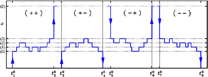
Figure 2: Schematic plots illustrating substeps and their counting rules (see text) in the $N=4$ case with $M=3$ for $(++)$, $(+-)$, $(-+)$, and $(--)$ stepping intervals. Thus, for example, from the first plot one confirms $n^{++}_{0,+}=n^{++}_{1,-}+1$ and, correspondingly, that the motor visited the state $[0]$ three times in this realization; and, likewise, $n^{++}_{1,+}+n^{++}_{1,-}=n^{++}_{0,+}+n^{++}_{2,-}$ is, here, equal to $4$ so that, correspondingly, the motor spent time in the substate $(1)$ on four occasions before undergoing the forward major transition $(3)\!\rightarrow\!(4\equiv 0)$. Similarly, the other plots serve to establish the frequency relations (112)-(121).

The frequency relations (112) and (113) with the boundary relations (114)-(121) constitute, together with the definition $\omega_{j}^{\rho\sigma}=(u_{j}+w_{j})T_{j}^{\rho\sigma}$ in (112), a complete set from which we may derive explicit general expressions for all the $n_{j,+}^{\rho\sigma}$ and $n_{j,-}^{\rho\sigma}$. To proceed, we note first that the purely counting arguments involving $\pi_{+}$, $\pi_{-}$, and $\pi_{++}$, $\pi_{--}$, etc., that led to the ‘reduced’ relations (56,57) and (59,60), apply equally to $\omega_{j}^{++}$, $\omega_{j}^{+-}$, etc. Accordingly, we obtain the post boundary frequency relations

$$\omega_{M+1}^{+\diamond} = n_{M+2,-}^{+\diamond}+1=n_{M+1,+}^{+\diamond}+\pi_{+-},$$ (122)

$$\omega_{M+N}^{+\diamond} = n_{M+N-1,+}^{+\diamond}=n_{M+N,-}^{+\diamond}+\pi_{++},$$ (123)

$$\omega_{M+1}^{-\diamond} = n_{M+2,-}^{-\diamond}=n_{M+1,+}^{-\diamond}+\pi_{--},$$ (124)

$$\omega_{M+N}^{-\diamond} = n_{M+N-1,+}^{-\diamond}+1=n_{M+N,-}^{-\diamond}+\pi_{-+},$$ (125)

while the prior relations are

$$\omega_{M+1}^{\diamond+} = n_{M+1,+}^{\diamond+}=n_{M+2,-}^{\diamond+}+\pi_{++},$$ (126)

$$\omega_{M+N}^{\diamond+} = n_{M+N,-}^{\diamond+}+1=n_{M+N-1,+}^{\diamond+}+\pi_{+-},$$ (127)

$$\omega_{M+1}^{\diamond-} = n_{M+1,+}^{\diamond-}+1=n_{M+2,-}^{\diamond-}+\pi_{-+},$$ (128)

$$\omega_{M+N}^{\diamond-} = n_{M+N,-}^{\diamond-}=n_{M+N-1,+}^{\diamond-}+\pi_{--},$$ (129)

Finally, in analogy to (61), we obtain

$$\omega_{M+1}^{\diamond\diamond} = n_{M+2,-}^{\diamond\diamond}+\pi_{+}=n_{M+1,+}^{\diamond\diamond}+\pi_{-},$$ (130)

$$\omega_{M+N}^{\diamond\diamond} = n_{M+N-1,+}^{\diamond\diamond}+\pi_{-}=n_{M+N,-}^{\diamond\diamond}+\pi_{+}.$$ (131)

Now (130) clearly implies the result

$$n_{M+1,+}^{\diamond\diamond}=\omega_{M+1}^{\diamond\diamond}-\pi_{-}=(u_{j}+w_{j})T_{M+1}^{\diamond\diamond}-\pi_{-},$$ (132)

where $\pi_{-}$ and $T_{M+1}^{\diamond\diamond}\equiv T_{M+1}^{\diamond\diamond}\!\left(\{u_{j},w_{j}\};M,N\right)$ are given explicitly in (77) and (95). A similar result follows from (130) for $n_{M+2,-}^{\diamond\diamond}$. But by appealing to (113) for $j=M+2$ we also obtain

$$n_{M+3,-}^{\diamond\diamond}=\omega_{M+2}^{\diamond\diamond}-n_{M+1,+}^{\diamond\diamond},$$ (133)

which, with the aid of (132), yields an explicit expression in terms of $T_{M+1}$ and $T_{M+2}$. Substituting $j=M+3$ in (112) then leads to an expression for $n_{M+3,+}^{\diamond\diamond}$. By proceeding recursively in this fashion we eventually obtain, for $k=1,2,\cdots$, the general expressions

$$n_{M+2k,-}^{\diamond\diamond}=\sum_{j=M+1}^{M+2k-1}(-)^{j-M-1}(u_{j}+w_{j})T_{j}^{\diamond\diamond}-\pi_{+},$$ (134)

$$n_{M+2k+1,-}^{\diamond\diamond}=\sum_{j=M+1}^{M+2k}(-)^{j-M}(u_{j}+w_{j})T_{j}^{\diamond\diamond}+\pi_{-},$$ (135)

for the average number of hidden back-substeps from the $N-2$ hidden intermediate states $(M+2)$ to $(M+N-1)$ and from the pre-step state $(M+N)\equiv(M)$. We may also note the sum rule

$$\sum_{l=0}^{N-1}(-)^{l}(u_{l}+w_{l})T^{\diamond\diamond}_{l}=\left\{\begin{array}[]{cccc}0&\mbox{for}&N&\mbox{even},\\ 1&\mbox{for}&N&\mbox{odd},\end{array}\right.$$ (136)

and the special relations $\pi_{+}=u_{M+N}T_{M+N}^{\diamond\diamond}$ and $\pi_{-}=w_{M+1}T_{M+1}^{\diamond\diamond}$, so that $n_{M+1,+}^{\diamond\diamond}=u_{M+1}T_{M+1}^{\diamond\diamond}$ and $n_{M+N,-}^{\diamond\diamond}=w_{M+N}T_{M+N}^{\diamond\diamond}$.

More generally (134) and (135) can be extended to arbitrary $(\rho,\sigma)$ if, following the sequence (107), $\pi_{+}$ and $\pi_{-}$ are replaced by

$$\tilde{\pi}_{+}=\{\pi_{+};\;1,0,\pi_{++},\pi_{-+};\;1,1,0,0\},$$ (137)

$$\tilde{\pi}_{-}=\{\pi_{-};\;\pi_{+-},\pi_{--},0,1;\;0,1,0,1\},$$ (138)

respectively. Finally, one finds that the mean number of forward substeps from the $N-2$ hidden intermediate states and the post-step state $(M+1)$ in specified intervals can be written

$$\!n_{M+2k,+}^{\rho\sigma}=\!\!\!\sum_{j=M+1}^{M+2k}\!\!\!(-)^{j-M}(u_{j}+w_{j})T_{j}^{\rho\sigma}+\tilde{\pi}_{+},$$ (139)

$$\!n_{M+2k-1,+}^{\rho\sigma}=\!\!\!\sum_{j=M+1}^{M+2k-1}\!\!\!(-)^{j-M-1}(u_{j}+w_{j})T_{j}^{\rho\sigma}-\tilde{\pi}_{-},$$ (140)

for $k=1,2,\cdots$. Some examples of these various expressions for small $N$ are listed in Appendix A.

IV Discussion and illustrations

First, it is appropriate to look more closely at the difference between our present results [see (76),(77), and (96)-(98)] and those of the previously published analysis kolomeisky03 ; kolomeisky05 . As in Sec. I [after (47)] we use a ha$\check{\textrm{c}}$ek to distinguish the results that presuppose the completion of a full enzymatic cycle between all pairs of successive major, i.e., observable steps. In the present notation one then has kolomeisky05

$$\check{\pi}_{+}=\frac{1}{1+\Gamma_{N}},\qquad\check{\pi}_{-}=\frac{\Gamma_{N}}{1+\Gamma_{N}},$$ (141)

for the forward/back fractions while the mean, prior, and post dwell times are all given by

$$\check{\tau}=\check{\tau}_{+}=\check{\tau}_{-}=\sum_{n=0}^{N-1}r_{n}\left/(1+\Gamma_{N})\right.,$$ (142)

where $r_{n}$ is defined in (68). On the other hand, when allowing for hidden substeps, these three times are all distinct: see (96)-(98).

Then, if one considers the average velocity defined by

$$V=d(\pi_{+}-\pi_{-})/\tau,$$ (143)

one finds that the result is the same in both cases, namely,

$$V=\check{V}=d(1-\Gamma_{N})\!\!\left/\mbox{$\sum_{n=0}^{N-1}$}r_{n}\right.,$$ (144)

as previously fisher99 ; kolomeisky03 ; fisher05 ; fisher99a ; kolomeisky00 . This is not really surprising, because the asymptotic ratio of the total distance to the total time should not depend on the way one takes into account (or ignores) substeps. Note that $\Gamma_{N}=1$ is the condition for stall, when $\pi_{+}=\pi_{-}$, in both analyses.

Now let us take a closer look at the ratio of splitting fractions, because this is a quantity which one can readily obtain from stepping observations to test theory. The effect of an external force, $\vec{F}=(F_{x},F_{y},F_{z})$, on the rates can be expressed in leading order fisher99 ; kim05 as

$$u_{l}=u^{0}_{l}\exp(+d\mbox{\boldmath$\theta$}^{+}_{l}\mbox{\boldmath$\cdot$}\,{\bf F}/k_{B}T),$$ (145)

$$w_{l}=w^{0}_{l}\exp(-d\mbox{\boldmath$\theta$}^{-}_{l}\mbox{\boldmath$\cdot$}\,{\bf F}/k_{B}T),$$ (146)

where $u^{0}_{l},w^{0}_{l}$ are the load-free rates while the load-distribution vectors $\mbox{\boldmath$\theta$}^{+}_{l}$ and $\mbox{\boldmath$\theta$}^{-}_{l}$ serve to specify how the $2N$ distinct rates respond to the stress. The periodicity of the stepping along the track (which we suppose is in the $x$ direction) implies

$$\sum_{n=0}^{N-1}\left(\mbox{\boldmath$\theta$}^{+}_{n}+\mbox{\boldmath$\theta$}^{-}_{n}\right)=\hat{\bf e}_{x}=(1,0,0).$$ (147)

Rearranging these relations leads to

$$\Gamma_{N} = \prod_{n=0}^{N-1}\frac{w_{n}}{u_{n}}=\exp\left(-\frac{dF_{x}}{k_{B}T}\right)\prod_{n=0}^{N-1}\frac{w^{0}_{n}}{u^{0}_{n}}$$ (148)

$$= \exp[-d(F_{x}-F_{S})/k_{B}T],$$

where the stall force is given by fisher99 ; kim05

$$F_{S}=\frac{k_{B}T}{d}\ln\left(\prod_{n=0}^{N-1}\frac{w^{0}_{n}}{u^{0}_{n}}\right).$$ (149)

From (141) we thus conclude

$$\ln(\check{\pi}_{+}/\check{\pi}_{-})=-\ln\Gamma_{N}=d(F_{x}-F_{S})/k_{B}T.$$ (150)

This is a strong prediction since it asserts that the logarithm of the stepping ratio $(\check{\pi}_{+}/\check{\pi}_{-})$ depends linearly on $F_{x}$ with a slope, $d/k_{B}T$, determined solely by the step size $d$. However, this result depends crucially on the assumption that the forward and back steps identified correspond to full enzymatic cycles (as the haceks indicate). In a typical experiment, however, the hidden substeps result in a violation of this assumption as we have explained.

Accordingly, let us, instead, compute the stepping fraction $(\pi_{+}/\pi_{-})$ for which (76) and (77) yield

$$\ln(\pi_{+}/\pi_{-})=d^{*}(F_{x}-F_{S})/k_{B}T,$$ (151)

where, for the sake of comparison with (150), we have introduced an effective step size

$$d^{*}=\frac{-k_{B}T}{F_{x}-F_{S}}\ln\left(\frac{\Gamma_{N}+\Delta_{M,N}}{1+\Delta_{M,N}}\right).$$ (152)

In general, this clearly depends on all the rates $\{u_{j},w_{j}\}$ and hence on the force $F_{x}$. In the special case $\Delta_{M,N}=0$, however, $d^{*}$ reduces [via (150)] to $d$. This condition is, in fact, realized when $N=1$ since $\Delta_{M,1}$ vanishes identically. But an $N=1$ model is unlikely to be adequate. Thus in real systems neither the full linearity vs. $F_{x}$ nor the equality $d^{*}=d$ are to be expected. In the vicinity of $F_{S}$, however, we can estimate $d^{*}$ by expanding in powers of $\delta F_{x}\equiv F_{x}-F_{S}$. This yields

$$\Gamma_{N}=1-d\,\delta F_{x}/k_{B}T+O(\delta F_{x}^{2}),$$ (153)

$$\Delta_{M,N}=\Delta_{S}+\Delta^{\prime}_{S}\delta F_{x}+O(\delta F_{x}^{2}),$$ (154)

where $\Delta_{S}=\Delta_{M,N}(F_{x}\!\!\,=\!F_{S})$ while $\Delta^{\prime}_{S}$ is the corresponding derivative. Thence we find

$$d^{*}=\frac{d}{1+\Delta_{S}}+O(\delta F_{x}).$$ (155)

It follows from the definition (67) that $\Delta_{S}$ cannot be negative so that, quite generally, one has $d^{*}\leqslant d$.

On the other hand, to be concrete, consider an ($N=2$, $M=1$) model for which we have

$$\!\!\Delta_{S} =(w_{0}/u_{0})_{S}=(u_{1}/w_{1})_{S}$$

$$=(u^{0}_{1}/w^{0}_{1})\exp\{d[F_{S}-(\mbox{\boldmath$\theta$}^{+}_{0}+\mbox{\boldmath$\theta$}^{-}_{0})\,\mbox{\boldmath$\cdot$}\,{\bf F}_{S}]/k_{B}T\},$$ (156)

where the subscript $S$ denotes evaluation at ${\bf F=F}_{S}=(F_{x}\!\!=\!F_{S},F_{y},F_{z})$ in which $F_{y}$ and $F_{z}$ need not vanish at stall kim05 . It is evident, that $\Delta_{S}$ is not bounded above so that $d^{*}/d$ is not bounded below. Indeed, the experiments on kinesin of Nishiyama et al. nishiyama03 and of Carter and Cross on kinesin carter05 lead to the estimates $d^{*}\simeq 3.2\;\mathrm{nm}$ and $d^{*}\simeq 4.0\;\mathrm{nm}$, respectively, whereas the step size is $d\simeq 8.2\;\mathrm{nm}$. This clearly indicates the importance of the hidden substeps in understanding the stepping fractions near stall.

As another concrete example we quote

$$\Delta_{S} = \left(\frac{w_{0}}{u_{0}}+\frac{w_{0}w_{1}}{u_{0}u_{1}}+\frac{w_{0}w_{1}w_{2}}{u_{0}u_{1}u_{2}}\right)_{S}$$ (157)

$$= \left(\frac{u_{1}u_{2}u_{3}}{w_{1}w_{2}w_{3}}+\frac{u_{2}u_{3}}{w_{2}w_{3}}+\frac{u_{3}}{w_{3}}\right)_{S},$$

for an ($N=4$, $M=3$) model. From this, however, one sees that $d^{*}$ will be close to $d$ if $(u_{3}/w_{3})_{S}$ and/or $(w_{0}/u_{0})_{S}$ are sufficiently small.

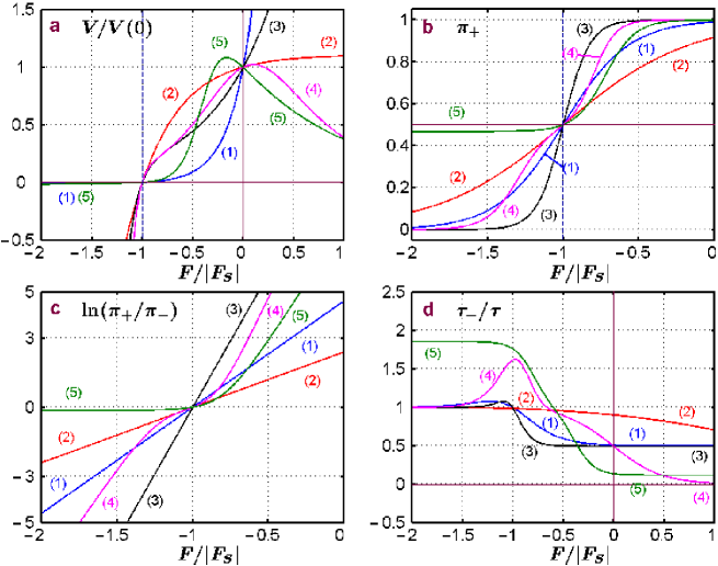
Figure 3: Plots illustrating different dependencies on the normalized force, $F/|F_{S}|$, of (a) the normalized velocity $V(F)/V(0)$; (b) the forward splitting fraction $\pi_{+}$; (c) the logarithm of the splitting fraction ratio $(\pi_{+}/\pi_{-})$; and (d) the ratio of mean prior backward to mean total dwell time, $\tau_{-}(F)/\tau(F)$. The individual plots, labeled (1) to (5), correspond to ($N=2$, $M=1$) models under scalar loading, $\textbf{F}\!=\!(F,0,0)$, with the selected parameter values presented in Table I.

More generally it seems likely that both the full cycle assumption and the hidden substep analysis should produce similar results when the rates, $u_{M}$ and $w_{M+1}$, for the major transition are slow relative to the substep rates. To demonstrate this explicitly let us suppose that the latter rates satisfy

$$u_{M}=\eta\,\tilde{u}_{M}\quad\mbox{and}\quad w_{M+1}=\eta\,\tilde{w}_{M+1},\\$$ (158)

where $\eta$ is small while $\tilde{u}_{M}$ and $\tilde{w}_{M+1}$ and all the substep rates, $u_{l}\equiv\tilde{u}_{l}$ $(l\neq M)$ and $w_{l}\equiv\tilde{w}_{l}$ $(l\neq M+1)$, are held fixed. Then one finds

$$\Gamma_{M,s}=\prod_{n=1}^{s}\frac{w_{M+n}}{u_{M+n}} = \eta\,\tilde{\Gamma}_{M,s}\quad\mbox{for}\quad s\in[1,N-1],$$ (159)

$$= \tilde{\Gamma}_{N}=\Gamma_{N}\quad\mbox{for}\quad s=N,$$

where $\tilde{\Gamma}_{M,s}=\prod_{n=1}^{s}(\tilde{w}_{M+n}/\tilde{u}_{M+n})$, and similarly, via (67),

$$\Delta_{M,N}=\eta\sum_{p=1}^{N-1}\tilde{\Gamma}_{M,p}\equiv\eta\tilde{\Delta}_{M,N}.$$ (160)

With the aid of these expressions we can rewrite the previous results (76,77) and (98) as

$$\pi_{+}=\frac{1+\eta\tilde{\Delta}_{M,N}}{1+\tilde{\Gamma}_{N}+2\eta\tilde{\Delta}_{M,N}}=1-\pi_{-},$$ (161)

$$\tau=\check{\tau}\frac{1+\tilde{\Gamma}_{N}}{1+\tilde{\Gamma}_{N}+2\eta\tilde{\Delta}_{M,N}}.$$ (162)

Evidently to zero order in $\eta$, the analyses are equivalent as anticipated.

As seen in earlier investigations that were confined to the velocity vs. force relation fisher99 ; fisher99a , a surprisingly wide range of behavior under varying loads is displayed even by the basic $(N=2)$-state models when the rates are subject to the exponential force distribution laws embodied in (145-147) fisher99 ; kim05 . This is illustrated in Fig.3(a) which depicts the velocity $V$, normalized by its value $V(0)$ under zero load, as a function of the imposed load $F$ (supposed parallel to the $x$-axis) normalized by the stall force magnitude $|F_{S}|$. The labeled plots (1) to (5) in Fig. 3 correspond to the selected parameter values listed in Table I. Note that superstall loads are included ($F/|F_{S}|<-1$) which for the parameter sets (1) and (5) results in only a relatively small negative velocity (as uncovered in the kinesin experiments of Carter and Cross carter05 ). Similarly, assisting loads ($F/|F_{S}|>0$) are also covered and for sets (2), (4), and (5) result in a saturating or, even, decreasing velocity under increasing load. In the substall resistively loaded region ($0>F/|F_{S}|>-1$) convex, concave, inflected, and even nonmonotonic [see parameter set (5)] behavior is realized.

For these different cases the corresponding forward stepping fractions $\pi_{+}(F)$ and the logarithmic ratios of forward/back steps, ($\pi_{+}/\pi_{-}$), are depicted in Figs. 3(b) and (c). [Note that in these figures only the resisting range of force, $F<0$, is displayed.] Although the variation is always monotonically increasing with $F$ (and $\pi_{+}=\pi_{-}=\frac{1}{2}$ when $F\!=\!F_{S}$), a wide range of forms is evident. In the logarithmic plot, Fig.3(c), one sees linear, concave, and inflected variation close to stall. Furthermore, the value of the effective step size $d^{*}$ varies markedly: see the last column in Table I.

By using the explicit expressions in the Appendix the nature of other statistical observables such as $\pi_{+-}(F)$, etc., is readily explored. Experiments often measure the overall mean dwell time, $\tau(F)$, between steps. Under assisting loads $(F>0)$, when $\pi_{-}$ is negligible, $\tau(F)$ directly mirrors the reciprocal of the velocity $V(F)$; but, in view of the factor $(\pi_{+}-\pi_{-})$ in (143), it varies somewhat differently under resisting loads. More interesting is the behavior of the partial dwell time $\tau_{-}(F)$ observed prior to back steps. This is shown in Fig. 3(d) normalized by the overall dwell time $\tau(F)=\pi_{+}\tau_{+}+\pi_{-}\tau_{-}$ [see (45)]. Even though, the ratio $\tau_{-}/\tau$ is confined to the range $(0,2)$ beyond superstall (since $\tau_{-}/\tau<1/\pi_{-}$ and $\pi_{-}>\frac{1}{2}$ for $V<0$), striking nonmonotonic and inflected variation arises.

Needless-to-say, many more plots exhibiting unexpected and surprising behavior can be generated; but further exploration seems most useful in connection with specific experimental data. Such applications are planned.

Table 1: Parameter values for ($N=2$, $M=1$) models under scalar loading, $F\equiv F_{x}$, employed in Fig. 3 to illustrate different force-dependencies. The last column presents the computed values of the effective step size $d^{*}$. [See (152).]

	$d|F_{S}|/k_{B}T$	$w^{0}_{0}/u^{0}_{0}$	$w^{0}_{1}/u^{0}_{0}$	$\theta^{+}_{1}$	$\theta^{-}_{0}=\theta^{-}_{1}$	$d^{*}/d$
(1)	9.2	10-2	10-2	0.5	0	0.501
(2)	2.5	10-2	10-2	0	0.5	0.966
(3)	23	10-5	10-5	0.07	0.43	0.503
(4)	23	10-5	10-5	$-$0.07	0.48	0.113
(5)	10	3.4$\times$10-4	2.5$\times$10-3	$-$0.1	0.1	0.118

V Multiple observed transitions

In the previous sections we have derived expressions only for the case of a single major transition in each enzymatic cycle; that, indeed, is the typical situation for experiments on conventional kinesin nishiyama02 ; block03 ; nishiyama03 ; carter05 . However, our results can be generalized to the case in which several substeps are sufficiently large to be clearly detected, while others remain hidden in the noise. Suppose there are $K$ visible substeps of (average) magnitudes $d_{A}$, $d_{B}$, $\cdots$, together totalling

$$d_{A}+d_{B}+\dots+d_{K}\simeq d,$$ (163)

that occur between states ($M_{J}$) and ($M_{J}+1$) with, in sequence,

$$0\leq M_{A}<M_{B}<\dots<M_{K}\leq N-1.$$ (164)

Then between states ($M_{J-1}+1$) and ($M_{J}$) there are $M_{J}-M_{J-1}$ hidden states and, consequently, all these states belong (within the noise) to what we may call the same mechanical level, $J$: see Fig. 4.

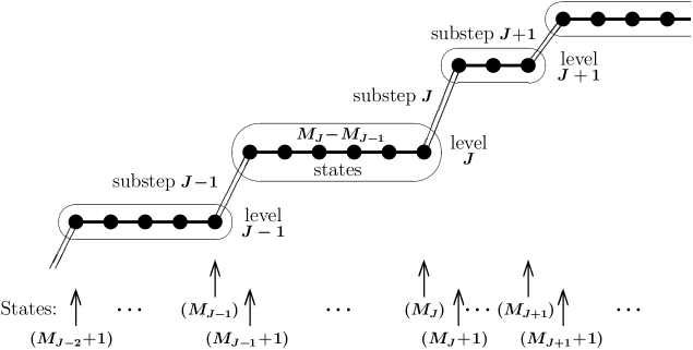
Figure 4: Schematic depiction of individual biochemical states, $(i)$, organized into mechanical levels, $A$, $B$, $\cdots$, $J-1$, $J$, $\cdots$ when there are $K>1$ detectable substeps or major transitions with substep $J$ going forward from state $(M_{J})$ to state $(M_{J}+1)$.

Now one can count all forward and backward detectable transitions in a long run. Accordingly, let $n^{J}_{++}$ be the number of pairs of observed substeps that enter the mechanical level $J$ via a $+$ transition, i.e., a step ($J-1$), and leave via a $+$ transition taking a step $J$, and similarly for $n^{J}_{+-}$, $n^{J}_{-+}$, and $n^{J}_{--}$. Then, as previously, we can estimate pairwise splitting fractions for level $J$ via

$$\pi^{J}_{++} = \frac{n^{J}_{++}}{n^{J}_{++}+n^{J}_{+-}}=1-\pi^{J}_{+-},$$ (165)

$$\pi^{J}_{-+} = \frac{n^{J}_{-+}}{n^{J}_{-+}+n^{J}_{--}}=1-\pi^{J}_{--}.$$ (166)

Likewise, we can introduce pair-wise dwell times, $\tau^{J}_{\rho\sigma}$, for each mechanical level $J$ as the mean times spent between a $\rho$ and $\sigma$ substep into and out of that level.

With these definitions we may adopt the same approach used in Sec. III by setting absorbing boundaries at states $(L)=(M_{J-1})$ and $(R)=(M_{J}+1)$ around each level $J$ and studying the appropriate first-passage processes. If we set

$$N_{J}=\; |M_{A}\!-\!M_{B}|,\;|M_{B}\!-\!M_{C}|,\;\cdots,$$

$$|M_{K}\!-\!M_{K-1}|,\;|N\!-\!M_{K}\!+\!M_{A}|,$$

$$\mbox{for}\quad J=A,\;B,\;\cdots,\;K-1,\;K,$$ (167)

we can then conclude, using the previous results (73,74), that

$$\pi^{J}_{\rho\sigma}=\pi_{\rho\sigma}(M_{J-1},N_{J-1}).$$ (168)

Similarly, recalling the definitions (84,85) for $T^{+}_{j}(M,N)$ and $T^{-}_{j}(M,N)$ and the results (90-93), we obtain

$$\tau^{J}_{\rho\sigma}=\tau_{\rho\sigma}(M_{J-1},N_{J-1}).$$ (169)

The counting of individual hidden substeps developed in Sec. III.5 can be carried forward to obtain the mean number of substep transitions between two specified major transitions. The results (134-140) essentially apply directly with $M\Rightarrow M_{J-1}$ and $N\Rightarrow N_{J-1}$.

In terms of the conditional individual state dwell times introduced in (102-104) we also have

$$\tau^{J}_{\rho\sigma}=\sum_{k=M_{J-1}+1}^{M_{J}}T_{k}^{\rho\sigma}(M_{J-1},N_{J-1}).$$ (170)

as a measure of the observable mean overall time spent in the mechanical level $J$ subject to the ($\rho,\sigma$) conditions.

As regards potential applications of these results, the case $K=2$ may be reasonable for a first analysis of data for myosin V where, as mentioned, a significant observable substep was originally predicted kolomeisky03 and later observed uemura04 ; however, the experiments also suggest uemura04 ; baker04 that stepping may proceed through two (or more) alternative pathways so that a purely sequential model (to which our attention has been restricted) may be inadequate foot0A . For the F₁-ATPase motor nishizaka04 ; shimabukuro03 ; ueno05 substeps have also been reported and occasional back steps have been observed. Thus our results should be applicable.

VI Summary and conclusion

As explained in the Introduction, the need to develop the hidden substep analysis we have presented arises from the fact that experimentally detectable steps in the motion of a motor protein along its track do not necessarily delineate the completion of full biochemical enzymatic cycles. As a consequence, previous analyses that addressed such observable statistics as back-stepping fractions, $\pi_{-}$, and mean dwell times, $\tau_{+}$ and $\tau_{-}$, measured prior to forward (or $+$) and back (or $-$) steps, were not adequate to relate the underlying rates in a biomechanochemical model, say $u_{i}$ and $w_{j}$ to the experimental data.

We have considered the basic $N$-state sequential kinetic model set out in (37) and specified by $N$ forward rates $u_{i}$ from biochemical state $(i)$ and $N$ reverse rates $w_{j}$ from state $(j)$. In general, the rates depend on the concentration of various reagents [see, e.g., (38)] and, in particular, vary experimentally with the load force ${\bf F}=(F_{x},F_{y},F_{z})$: see (145,146).

The basic problem may then be set up by supposing that as the motor progresses (or retrogresses) along its molecular track only a single “major transition” from state $(M)$ to $(M+1)$ $\>(0\leq M<N)$, or its reverse, corresponds to a “visible” or detectable “step” in the $N$-state cycle. All the other transitions are “hidden”: see Fig. 1. [Cases in which more than one major transition or observable (sub)step occur in each full enzymatic cycle are analyzed in Sec. V.] It then transpires that two crucial combinations of the rates $\{u_{i},w_{j}\}$ play a central role, namely, $\Gamma_{N}$ and $\Delta_{M,N}$ as defined in (65)-(67).

Indeed, explicit expressions for the forward and backward stepping fractions, $\pi_{+}$ and $\pi_{-}$, are derived in terms of $\Gamma_{N}$ and $\Delta_{M,N}$ in Sec. III.2 and presented in (76) and (77). It proves helpful, furthermore, to relate $\pi_{+}$ and $\pi_{-}$ to the conditional or pairwise step probabilities, $\pi_{++}$, $\pi_{+-}$, etc., for $+$ steps followed by a $+$ step, or by a $-$ step, etc., that can be defined via counting observations, as explained in (51)-(54) and the associated text. These pairwise probabilities are likewise expressible in terms of $\Gamma_{N}$ and $\Delta_{M,N}$: see (73) and (74).

From these results one can see – as explained in further detail in Sec. IV – that only when $\;\Delta_{M,N}\ll\min\{1,\Gamma_{N}\}\;$ can one neglect the hidden substeps without risk of serious error. Particularly instructive is the variation of $\;\ln(\pi_{+}/\pi_{-})\;$ as the load $F_{x}$ passes through stall (at which $\;\pi_{+}=\pi_{-}=\frac{1}{2}\;$ so that the mean velocity vanishes). One may then define an effective step length, $d^{*}$, via (151) and (152). When $\Delta_{M,N}\rightarrow 0$ (or if hidden substeps are ignored) one has the simple equality $\;d^{*}=d$, where $d$ is the full step size of the motor (per cycle). But, in fact, $d^{*}/d$ must always be less than unity and, as seen in experiment and illustrated in Table I, this ratio is typically of magnitude only 0.3 to 0.5.

Going beyond simple counts of backward and forward steps, one may also define conditional mean dwell times, $\tau_{++}$, $\tau_{+-}$, etc., for the time spent between a pair of successive $+$ steps, or a $+$ step followed by a $-$ step, etc.: see (48). These pairwise mean times can likewise be calculated [see (90) to (93)] in terms of individual-state post dwell times, $T_{j}^{+}(\equiv T_{j}^{+\diamond})$ and $T_{j}^{-}(\equiv T_{j}^{-\diamond})$, that represent the mean time spent in a state $(j)$ following a $+$ or $-$ step, respectively: see Sec. III.4 for a fuller explanation of the notation, etc. The corresponding explicit expressions, (84) and (85), involve the basic rate products $\Gamma_{l,m}$ and their sums, $\Delta_{l,n}$, as again defined in (65) and (67). The final results for $\tau_{+}$, $\tau_{-}$, and for the overall mean dwell time $\tau$ (between $+$ or $-$ steps) for general $M$ and $N$ entail slightly simpler sums: see (95)-(98).

More transparent formulae for the stepping fractions and dwell times for $N=2$ models (involving only the rates $u_{0}$, $u_{1}$, $w_{0}$, and $w_{1}$,) and for selected $N=4$ models, are presented in Appendix A. In addition, the parts of Fig. 3 and the associated discussion in Sec. IV, illustrate that a wide range of different types of behavior of $\pi_{+}(F)$, $\ln[\pi_{+}(F)/\pi_{-}(F)]$, and $\tau_{-}(F)$ as functions of load can be realized even within simple $N=2$ models.

At a higher level of detail, conditional individual-state dwell times, $T_{j}^{++}$, $T_{j}^{+-}$, $\cdots$, can be derived [see (102)-(104)] and, likewise, post (as against the previously mentioned prior) dwell times, $\tau_{+\diamond}$ and $\tau_{-\diamond}$: see (100). Finally, one can obtain the expressions (134), (135), (139), and (140), for the mean number, $n_{j,+}^{\rho\sigma}$ and $n_{j,-}^{\rho\sigma}$ of hidden, forwards and backwards, substeps from an individual state $(j)$ that occur in a time interval between detectable steps, i.e., major transitions specified by $\{\rho,\sigma\}=\{\cdots,+-,-+,\cdots\}$: see (107). These results provide quantitative estimates for the number of “lost” or “hidden” transitions occurring in an enzymatic cycle. Such information could be of particular interest for real motor proteins since, when operating in cells to achieve mitosis, etc., they may frequently be in close-to-stall conditions where reverse substeps are likely to be most frequent grill03 ; pecreaux06 .

In conclusion, we have provided a detailed analysis of the statistics of mechanochemical transitions that must be hidden in the experimental noise when a motor protein on its track moves processively via distinct steps, or reaches stall. As experimental resolution at the microsecond and nanometer scales improves, we can expect that such analyses will be increasingly valuable for extracting reliable inferences about motor mechanisms from observational data.

Appendix A   Expressions for Two-State and Four-State Models

For convenience of reference we provide here explicit expressions for $N=2$ models with $M=1$. First, we recall the full-cycle expressions kolomeisky03 ; kolomeisky05

$$\check{\pi}_{+}=1-\check{\pi}_{-}=\frac{u_{0}u_{1}}{u_{0}u_{1}+w_{0}w_{1}},$$ (171)

$$\check{\tau}_{+}=\check{\tau}_{-}=\check{\tau}=\frac{u_{0}+u_{1}+w_{0}+w_{1}}{u_{0}u_{1}+w_{0}w_{1}},$$ (172)

the result for general $N$ being given in (141),(142). Allowing for hidden substeps leads to

$$\pi_{+}=1-\pi_{-}=\frac{u_{1}(u_{0}+w_{0})}{u_{0}u_{1}+w_{0}w_{1}+2u_{1}w_{0}},$$ (173)

while the distinct prior dwell (or stepping) times are given by

$$\tau_{+}\equiv\tau_{\diamond+}=\frac{(u_{0}+w_{0})^{2}+u_{0}(u_{1}+w_{1})}{(u_{0}+w_{0})(u_{0}u_{1}+w_{0}w_{1}+u_{1}w_{0})},$$ (174)

$$\tau_{-}\equiv\tau_{\diamond-}=\frac{(u_{1}+w_{1})^{2}+w_{1}(u_{0}+w_{0})}{(u_{1}+w_{1})(u_{0}u_{1}+w_{0}w_{1}+u_{1}w_{0})},$$ (175)

with the mean overall dwell time

$$\tau=\pi_{+}\tau_{+}+\pi_{-}\tau_{-}=\frac{u_{0}+u_{1}+w_{0}+w_{1}}{u_{0}u_{1}+w_{0}w_{1}+2u_{1}w_{0}}.$$ (176)

For general $N$ see (76), (77), and (96)-(98).

The partial or conditional pairwise step probabilities follow, by specializing (73) and (74), as

$$\pi_{++}=1-\pi_{+-}=\frac{u_{0}u_{1}}{u_{0}u_{1}+w_{0}w_{1}+u_{1}w_{0}},$$ (177)

$$\pi_{-+}=1-\pi_{--}=\frac{u_{1}(u_{0}+w_{0})}{u_{0}u_{1}+w_{0}w_{1}+u_{1}w_{0}}.$$ (178)

The denominators here, say

$$\mathfrak{D}_{2}=u_{0}u_{1}+w_{0}w_{1}+u_{1}w_{0},$$ (179)

should be contrasted with those in (173) and (176), namely,

$$\mathfrak{D}^{+}_{2}=\mathfrak{D}_{2}+u_{1}w_{0}=u_{0}u_{1}+w_{0}w_{1}+2u_{1}w_{0}.$$ (180)

At the next level of individual (or partial) (sub)state properties, the individual or substate dwell times follow from (95), which yields

$$T_{0}=(u_{1}+w_{1})/\mathfrak{D}^{+}_{2},\qquad T_{1}=(u_{0}+w_{0})/\mathfrak{D}^{+}_{2},$$ (181)

which, in accord with (98), satisfy $\tau=T_{0}+T_{1}$. The partial substate dwell times, given generally in (84,85), are

$$T_{0}^{+}=(u_{1}+w_{1})/\mathfrak{D}_{2},\mathfrak{\qquad}T_{1}^{+}=u_{0}/\mathfrak{D}_{2},$$ (182)

$$T_{0}^{-}=w_{1}/\mathfrak{D}_{2},\mathfrak{\qquad}T_{1}^{-}=(u_{0}+w_{0})/\mathfrak{D}_{2}.$$ (183)

Finally, the conditional or pairwise mean dwell or stepping times are

$$\tau_{++} = \tau_{--}=(u_{0}+u_{1}+w_{0}+w_{1})/\mathfrak{D}_{2},$$ (184)

$$\tau_{+-} = [(u_{1}+w_{1})^{2}+u_{0}w_{1}]/(u_{1}+w_{1})\mathfrak{D}_{2},$$ (185)

$$\tau_{-+} = [(u_{0}+w_{0})^{2}+u_{0}w_{1}]/(u_{0}+w_{0})\mathfrak{D}_{2}.$$ (186)

The mean numbers of hidden transitions follow from the results in Sec. III.5. For the simplest $N=2$ ($M=1$) case we obtain

$$n_{0,+}^{++}-1 =n_{0,+}^{+-}=n_{0,+}^{-+}=n_{0,+}^{--}=n_{0,+}^{-\diamond}$$

$$=n_{0,+}^{\diamond-}=n_{1,-}^{++}=n_{1,-}^{+-}=n_{1,-}^{-+}$$

$$=n_{1,-}^{--}-1=n_{1,-}^{+\diamond}=n_{1,-}^{\diamond+}=u_{0}w_{1}/\mathfrak{D}_{2},$$ (187)

$$n_{0,+}^{+\diamond} =n_{0,+}^{\diamond+}=u_{0}(u_{1}+w_{1})/\mathfrak{D}_{2},$$ (188)

$$n_{1,-}^{-\diamond} =n_{1,-}^{\diamond-}=w_{1}(u_{0}+w_{0})/\mathfrak{D}_{2},$$ (189)

$$n_{0,+}^{\diamond\diamond} =u_{0}(u_{1}+w_{1})/\mathfrak{D}^{+}_{2},$$ (190)

$$n_{1,-}^{\diamond\diamond} =w_{1}(u_{0}+w_{0})/\mathfrak{D}^{+}_{2}.$$ (191)

To provide further insight we quote some results for $N=4$ models with $M=3$, i.e., with the major step as the last transition from state (3) to $[4\equiv 0]$. Thus we have

$$\pi_{-}=w_{0}\mathfrak{N}_{0}/\mathfrak{D}^{+}_{4},\qquad\pi_{+}=u_{3}\mathfrak{N}_{3}/\mathfrak{D}^{+}_{4},$$ (192)

$$\tau=(\mathfrak{N}_{0}+\mathfrak{N}_{1}+\mathfrak{N}_{2}+\mathfrak{N}_{3})/\mathfrak{D}^{+}_{4},$$ (193)

where, to write the numerator and denominator contributions compactly, we introduce the short-hand product notation

$$u_{0,1}=u_{0}u_{1},\;u_{0,1,2}=u_{0}u_{1}u_{2},\;\cdots,$$

$$w_{0,1}=w_{0}w_{1},\;w_{0,1,2}=w_{0}w_{1}w_{2},\;\cdots,$$ (194)

etc. Then we have

$$\mathfrak{N}_{0} = u_{1,2,3}+w_{1}u_{2,3}+w_{1,2}u_{3}+w_{1,2,3},$$ (195)

$$\mathfrak{N}_{1} = u_{2,3,0}+w_{2}u_{3,0}+w_{2,3}u_{0}+w_{2,3,0},$$ (196)

$$\mathfrak{N}_{2} = u_{3,0,1}+w_{3}u_{0,1}+w_{3,0}u_{1}+w_{3,0,1},$$ (197)

$$\mathfrak{N}_{3} = u_{0,1,2}+w_{0}u_{1,2}+w_{0,1}u_{2}+w_{0,1,2},$$ (198)

while the denominator is given by

$$\mathfrak{D}^{+}_{4} = w_{0}\mathfrak{N}_{0}+u_{3}\mathfrak{N}_{3}=u_{0,1,2,3}+2w_{0}u_{1,2,3}$$ (199)

$$+ 2w_{0,1}u_{2,3}+2w_{0,1,2}u_{3}+w_{0,1,2,3}.$$

For the purpose of comparison we quote the result for the velocity, namely,

$$V=d(u_{0,1,2,3}-w_{0,1,2,3})/(\mathfrak{N}_{0}+\mathfrak{N}_{1}+\mathfrak{N}_{2}+\mathfrak{N}_{3}),$$ (200)

which, of course, is not simply $d/\tau$: see (143). Finally, then we also quote

$$\tau_{++}=\tau_{--} =[\mathfrak{N}_{0}+\mathfrak{N}_{1}+\mathfrak{N}_{2}+\mathfrak{N}_{3}$$

$$+w_{0}u_{3}(u_{1}+w_{1}+u_{2}+w_{2})]/\mathfrak{D}_{4},$$ (201)

and

$$\tau_{+}=\frac{u_{2,1,0}\mathfrak{N}_{0}+u_{2,1}\mathfrak{D}_{1}\mathfrak{N}_{1}+u_{2}\mathfrak{D}_{2}\mathfrak{N}_{2}+\mathfrak{D}_{3}\mathfrak{N}_{3}}{\mathfrak{D}_{4}\mathfrak{N}_{3}},$$ (202)

where

$$\mathfrak{D}_{N} =u_{0,1,\cdots,N-1}+w_{0}u_{1,2,\cdots,N-1}$$

$$+w_{0,1}u_{2,3,\cdots,N-1}+\cdots+w_{0,1,\cdots,N-1},$$ (203)

from which $\tau_{-}$ follows by using $\pi_{-}\tau_{-}+\pi_{+}\tau_{+}=\tau$. Of course, results for $M=0$, $1$, and $2$ and for $\pi_{++}$, $\tau_{++}$, $T_{j}$, etc., follow from the expressions derived in Sec. III.

References

- (1) J. Howard, Mechanics of Motor Proteins and the Cytoskeleton (Sinauer, Sunderland, 2001).
- (2) D. Bray, Cell Movements: From Molecules to Motility (Garland, New York, 2001).
- (3) A. D. Mehta, R. S. Rock, M. Rief, J. A. Spudich, M. S. Mooseker, and R. E. Cheney, Nature 400, 590 (1999).
- (4) M. Rief, R. S. Rock, A. D. Mehta, M. S. Mooseker, R. E. Cheney, and J. A. Spudich, Proc. Natl. Acad. Sci. USA 97, 9482 (2000).
- (5) M. Nishiyama, H. Higuchi, and T. Yanagida, Nature Cell Biol. 4, 790 (2002).
- (6) S. M. Block, C. L. Asbury, J. W. Shaevitz, and M. J. Lang, Proc. Natl. Acad. Sci. USA 100, 2351 (2003).
- (7) M. Nishiyama, H. Higuchi, Y. Ishii, Y. Taniguchi, and T. Yanagida, Biosystems 71, 145 (2003).
- (8) A. Yildiz, M. Tomishige, R. D. Vale, and P. R. Selvin, Science 303, 676 (2004).
- (9) G. E. Snyder, T. Sakamoto, J. A. Hammer, III, J. R. Sellers, and P. R. Selvin, Biophys. J. 87, 1776 (2004).
- (10) S. Uemura, H. Higuchi, A. O. Olivares, E. M. De La Cruz, and S. Ishiwata, Nat. Struct. Mol. Biol. 11, 877 (2004).
- (11) J. E. Baker, E. B. Krementsova, G. G. Kennedy, A. Armstrong, K. M. Trybus, and D. M. Warshaw, Proc. Natl Acad. Sci. USA 101, 5542 (2004).
- (12) K. Oiwa and H. Sakakibara, Curr. Opin. Cell Biol. 17, 98 (2005).
- (13) N. J. Carter and R. A. Cross, Nature 435, 308 (2005).
- (14) Y. Taniguchi, M. Nishiyama, Y. Ishii, and T. Yanagida, Nat. Chem. Biol. 1, 342 (2005).
- (15) A. E.-M. Clemen, M. Vilfan, J. J. Junshan Zhang, M. Bärmann, and M. Rief, Biophys. J. 88, 4401 (2005).
- (16) N. R. Guydosh and S. M. Block, Proc. Natl Acad. Sci. USA 103, 8054 (2006).
- (17) S. Toba, T. M. Watanabe, L. Yamaguchi-Okimoto, Y. Y. Toyoshima, and H. Higuchi, Proc. Natl Acad. Sci. USA 103, 5741 (2006).
- (18) See, e.g., M. E. Fisher and A. B. Kolomeisky, Proc. Natl Acad. Sci. USA 96, 6597 (1999); ibid. 98, 7748 (2001).
- (19) A. B. Kolomeisky and M. E. Fisher, Biophys. J. 84, 1642 (2003).
- (20) M. E. Fisher and Y. C. Kim, Proc. Natl Acad. Sci. USA 102, 16209 (2005).
- (21) M. E. Fisher and A. B. Kolomeisky, Physica A 274, 241 (1999).
- (22) A. B. Kolomeisky and M. E. Fisher, Physica A 279, 1; 284, 496 (2000).
- (23) Y. C. Kim and M. E. Fisher, J. Phys.: Condens. Matter 17, S3821 (2005).
- (24) C. Bustamante, D. Keller and G. Oster, Acc. Chem. Res. 34, 412 (2001).
- (25) It may be remarked parenthetically that, likewise, each biochemical transition proceeds via a chemical transition state, say , with -coordinate, say, . Thus, in turn, partial substeps of magnitudes and may be defined and, in principle, could be detectable. They satisfy kim05 .
- (26) It should be noted that K. I. Skau, R. B. Hoyle, and M. S. Turner, Biophys. J. 91, 2475 (2006), have presented a specific analytic treatment of backstep fractions in myosin V allowing for the two observed substeps in a full stepping cycle. Their approach differs from ours and, in particular, they do not seek statistical information regarding the detectable substeps separately.
- (27) R. Yasuda, H. Noji, K. Kinosita Jr., and M. Yoshida, Cell 93, 1117 (1998).
- (28) K. Shimabukuro, R. Yasuda, E. Muneyuki, K. Y. Hara, K. Kinosita Jr., and M. Yoshida, Proc. Natl Acad. Sci. USA 100, 14731 (2003).
- (29) T. Nishizaka, K. Oiwa, H. Noji, S. Kimura, E. Muneyuki, M. Yoshida, and K. Kinosita Jr, Nat. Struct. Mol. Biol. 11, 142 (2004).
- (30) K. Shimabukuro, E. Muneyuki, and M. Yoshida, Biophys. J. 90, 1028 (2005).
- (31) M. Diez, B. Zimmermann, M. Börsch, M. König, E. Schweinberger, S. Steigmiller, R. Reuter, S. Felekyan, V. Kudryavtsev, C. A. M. Seidel, and P. Gräber, Nat. Struct. Mol. Biol. 11, 135 (2004).
- (32) H. Ueno, T. Suzuki, K. Kinosita Jr., and M. Yoshida, Proc. Natl Acad. Sci. USA 102, 1333 (2005).
- (33) Y. Sowa, A. D. Rowe, M. C. Leake, T. Yakushi, M. Homma, A. Ishijima, and R. M. Berry, Nature 437, 916 (2005).
- (34) A. B. Kolomeisky, E. B. Stukalin, and A. A. Popov, Phys. Rev. E, 71, 031902 (2005).
- (35) H. Qian and X. S. Xie, Phys. Rev. E 74, 010902 (2006).
- (36) H. Wang and H. Qian, [to be published].
- (37) N. G. van Kampen, Stochastic Processes in Physics and Chemistry, Revised Edition (Elsevier, Amsterdam, 1992).
- (38) C. Veigel, S. Schmitz, F. Wang, and J. R. Sellers, Nature Cell Biol. 7, 861 (2005).
- (39) D. A. Smith, W. Steffen, R. M. Simmons, and J. Sleep, Biophys. J. 81, 2795 (2001).
- (40) L. S. Milescu, A. Yildiz, P. R. Selvin, and F. Sachs, Biophys. J. 91, 1156 (2006).
- (41) S. A. McKinney, C. Joo, and T. Ha, Biophys. J. 91, 1941 (2006).
- (42) L. S. Milescu, A. Yildiz, P. R. Selvin, and F. Sachs, Biophys. J. 91, 3135 (2006).
- (43) For reviews and other applications of hidden Markov processes in gene expression, communication theory, etc., see O. Zuk, I. Kanter, and E. Domany, J. Stat. Phys. 121, 343 (2005) and references therein.
- (44) Note that a related but distinct notation was used in Ref. kolomeisky00 and in A. B. Kolomeisky and M. E. Fisher, J. Chem. Phys. 113, 10867 (2000): specifically the products were defined along with , where is defined in (65).
- (45) S. W. Grill, J. Howard, E. Schäffer, E. H. K. Stelzer, and A. A. Hyman, Science 301, 518 (2003).
- (46) J. Pecreaux, J.-C. Röper, K. Kruse, F. Jülicher, A. A. Hyman, S. W. Grill, and J. Howard, Current Biology 16, 1 (2006).