An individual-based predator-prey model for biological coevolution: Fluctuations, stability, and community structure

Abstract

We study an individual-based predator-prey model of biological coevolution, using linear stability analysis and large-scale kinetic Monte Carlo simulations. The model exhibits approximate $1/f$ noise in diversity and population-size fluctuations, and it generates a sequence of quasi-steady communities in the form of simple food webs. These communities are quite resilient toward the loss of one or a few species, which is reflected in different power-law exponents for the durations of communities and the lifetimes of species. The exponent for the former is near $-1$, while the latter is close to $-2$. Statistical characteristics of the evolving communities, including degree (predator and prey) distributions and proportions of basal, intermediate, and top species, compare reasonably with data for real food webs.

I Introduction

Biological evolution presents many problems concerning interacting multi-entity systems far from equilibrium that are well suited for methods from nonequilibrium statistical physics Baake and Gabriel (2000); Drossel (2001). Among these are questions concerning the dynamics of the emergence and extinction of species on macroevolutionary timescales Newman and Sibani (1999); Newman and Palmer (2003); Bornholdt et al. . Traditionally it has been common to treat ecological and evolutionary processes on very different timescales. However, it has recently been realized that evolution often can take place on short timescales, comparable to those of ecological processes Thompson (1998, 1999); Drossel et al. (2001); Yoshida et al. (2003). A well-known example of very rapid evolution is provided by the cichlid fishes of East Africa Kocher (2004). Several models have therefore been proposed that, while spanning disparate scales of temporal and taxonomic resolution, consider the complex problem of coevolution of species in a fitness landscape that constantly changes with the composition of the community. Early contributions were simulations of parapatric and sympatric speciation Crosby (1970) and the coupled $NK$ model with population dynamics Kauffman and Johnsen (1991); Kauffman (1993). More recent work includes the Webworld model Caldarelli et al. (1998); Drossel et al. (2001, 2004), the tangled-nature model Christensen et al. (2002); Hall et al. (2002); di Collobiano et al. (2003) and simplified versions of the latter Rikvold and Zia (2003); Zia and Rikvold (2004); Sevim and Rikvold (2005), as well as network models Chowdhury et al. (2003); Chowdhury and Stauffer (2005). Recently, large individual-based simulations have also been performed of parapatric and sympatric speciation Gavrilets and Boake (1998); Gavrilets et al. (2000) and of adaptive radiation Gavrilets and Vose (2005).

Many of the models discussed above are deliberately quite simple, aiming to elucidate universal features that are largely independent of the finer details of the ecological interactions and the evolutionary mechanisms. Such features may include lifetime distributions for species and communities, as well as other aspects of extinction statistics, statistical properties of fluctuations in diversity and population sizes, and the structure and dynamics of food webs that develop and change with time.

In the present paper we continue our study of a simplified version of the tangled-nature model. In the early studies of this individual-based model of coevolution Rikvold and Zia (2003); Zia and Rikvold (2004); Sevim and Rikvold (2005), the interspecies interactions, which are described by an interaction matrix $\bf M$ Solé et al. (1996), were random and could produce any combination of pair interactions: favorable-favorable, deleterious-deleterious, or favorable-deleterious. Under those conditions the model was found to evolve through a sequence of quasi-stable communities, in which all species interact with mutually favorable interactions, i.e., mutualistic or symbiotic communities. For that reason we shall hereafter refer to that version of the model as the mutualistic model. Here we instead concentrate on a version that specifically describes the evolution of predator-prey communities. This restriction is enforced by means of an antisymmetric interaction matrix, so that an interaction that is favorable for one member of a pair is deleterious for the other, and vice versa. Many aspects of the dynamics of this predator-prey model are similar to the mutualistic model, such as approximate $1/f$ noise in species diversity and population sizes, and power-law distributions of the durations of communities and the lifetimes of species. However, some of the power-law exponents are different, and, most importantly, the predator-prey model produces communities that take the form of simple food webs. It also shares with the mutualistic model the property that mean population sizes and stability properties of fixed-point communities can be calculated exactly in the absence of mutations. Comparisons of some aspects of the predator-prey model (with a much smaller number of potential species than used here) to those of the mutualistic model have been presented in Refs. Rikvold (2005, a). The focus of the present paper is a much more detailed discussion of the dynamics and the structure of the resulting food webs (including comparison with real food webs) for the predator-prey model with a large number of potential species. For this purpose we use both exact linear-stability analysis and large-scale kinetic Monte Carlo simulations. In particular we wish to study the fluctuations in the statistically stationary state that develops for long times. A motivation is the hope that understanding of these stationary-state fluctuations can provide information about the system’s sensitivity to external perturbations in a way analogous to a fluctuation-dissipation relation Sato et al. (2003). We therefore carry out very long simulations.

The rest of this paper is organized as follows. The model is presented in Sec. II. Exact linear-stability analysis is performed in Sec. III, including fixed-point population sizes in Sec. III.1 and stability considerations in Sec. III.2. Numerical results are presented in Sec. IV, including species abundance distributions and time series of diversities and population sizes (Sec. IV.1), power spectral densities (Sec. IV.2), species lifetimes (Sec. IV.3), durations of evolutionarily quiet and active periods (Sec. IV.4), and community structure and stability with comparison with real food webs (Sec. IV.5). Our conclusions are summarized in Sec. V, and the method used to calculate the interaction matrices for systems with a large number of potential species is explained in Appendix A.

II Model

The model considered here is a version of the macroevolution model introduced by Rikvold and Zia Rikvold and Zia (2003) as a simplification of the tangled-nature model of Jensen and coworkers Hall et al. (2002); Christensen et al. (2002); di Collobiano et al. (2003). In this version, the interspecies interactions are constrained to represent a pure predator-prey system. As in Ref. Rikvold and Zia (2003), selection is provided by the reproduction rates in an individual-based, simplified multispecies population-dynamics model with nonoverlapping generations. This interacting birth/death process is augmented to enable evolution of new species by a mutation mechanism. The mutations act on a haploid, binary “genome” of length $L$, as introduced by Eigen for molecular evolution Eigen (1971); Eigen et al. (1988). This bit string defines the species, which are identified by the integer label $I\in[0,2^{L}-1]$. Typically, only a few of these $2^{L}$ potential species are resident in the community at any one time.

During reproduction, an offspring individual may undergo a mutation that flips a randomly chosen gene ($0\rightarrow 1$ or $1\rightarrow 0$) with a small probability, $\mu$. The mutation thus corresponds to diffusional moves from corner to corner along the edges of an $L$-dimensional hypercube Gavrilets (1999, 2004). A mutated individual is assumed to belong to a different species than its parent, with different properties. Genotype and phenotype are thus in one-to-one correspondence in this model. This is clearly a highly idealized picture, and it is introduced to maximize the pool of different species available within the computational resources. This picture is justified by a large-scale computational study of the mutualistic version of the model studied in Ref. Rikvold and Zia (2003), in which species that differ by as many as $L/2$ bits have correlated properties Sevim and Rikvold (2005). Remarkably, this study reveals that the more realistic, correlated model has long-time dynamical properties very similar to the uncorrelated model.

The reproduction probability $P_{I}(t)$ for an individual of species $I$ in generation $t$ depends on the individual’s ability to utilize the amount $R$ of available external resources, and on its interactions with the population sizes $n_{J}(t)$ of all the species present in the community at that time. The dependence of $P_{I}$ on the set of $n_{J}$ is determined by an interaction matrix $\bf M$ Solé et al. (1996) with offdiagonal elements ${M}_{IJ}$ that are continuously and symmetrically distributed on the interval $[-1,+1]$ in a way defined specifically in the next paragraph. The elements of $\bf M$ are chosen randomly at the beginning of each simulation run and are subsequently kept constant throughout the run (quenched randomness). (For a discussion of how the matrix elements are created for $L>13$, in which case the $2^{L}\times 2^{L}$ matrix does not fit into the memory of a standard workstation, see Appendix A. This method leads to a distribution that is triangular on $[-1,+1]$.)

In contrast to our previously studied model Rikvold and Zia (2003); Zia and Rikvold (2004); Sevim and Rikvold (2005), in which the interaction matrix has no particular structure, the predator-prey dynamics is enforced by the requirement that the off-diagonal part of $\bf M$ must be antisymmetric. Thus, if $M_{IJ}>0$ and $M_{JI}<0$, then species $I$ is the predator and $J$ the prey, and vice versa. In order to keep the connectance of the resulting communities consistent with food webs observed in nature Dunne et al. (2002a); Garlaschelli (2004) the $(M_{IJ},M_{JI})$ pairs are chosen nonzero with probability $c=0.1$. The nonzero elements in the upper triangle of $\bf M$ are chosen independently from the triangular distribution on $[-1,+1]$, described in Appendix A. Self-competition is included in the model by choosing the diagonal elements of $M$ randomly and uniformly from $[-1,0)$.

The reproduction probability for species $I$, $P_{I}(t)$, depends on $R$ and the set $\{n_{J}(t)\}$ through the nonlinear form,

$$P_{I}(t)=\frac{1}{1+\exp[-\Delta_{I}(R,\{n_{J}(t)\})]}\;,$$ (1)

where

$$\Delta_{I}(R,\{n_{J}(t)\})=-b_{I}+\eta_{I}R/N_{\rm tot}+\sum_{J}M_{IJ}n_{J}(t)/N_{\rm tot}\;.$$ (2)

Here $b_{I}$ is the “cost” of reproduction for species $I$ (always positive), and $\eta_{I}$ (positive for primary producers or autotrophs, and zero for consumers or heterotrophs) is the ability of individuals of species $I$ to utilize the external resource $R$. The latter is renewed at the same level every generation and does not have independent dynamics. The total population size is $N_{\rm tot}(t)=\sum_{J}n_{J}(t)$. [In contrast, the total number of species present in generation $t$ (the species richness) will be defined as $\mathcal{N}(t)$.] The population-limiting reproduction costs $b_{I}$ are chosen randomly and uniformly from the interval $(0,+1]$. Only a proportion $p$ of the $2^{L}$ potential species are producers that can directly utilize the resource. (For the numerical data shown here, we use $p=0.05$.) Thus, with probability $(1-p)$ the resource coupling $\eta_{I}=0$, representing consumers, while with probability $p$ the $\eta_{I}$ are independently and uniformly distributed on $(0,+1]$, representing producers of varying efficiency. In addition to the constraints on $\bf M$ mentioned above, we require that producers always are the prey of consumers. Thus, the case $\eta_{I}>0$ and $\eta_{J}=0$ with $M_{IJ}\equiv-M_{JI}>0$ is forbidden and is changed during setup of the matrix by reversing the signs of the interactions for the pair in question.

For large positive $\Delta_{I}$, (small birth cost, strong coupling to the external resources, and more prey than predators), the individual almost certainly reproduces, giving rise to $F$ offspring. In the opposite limit of large negative $\Delta_{I}$, (large birth cost, weak or no coupling to the external resources, and/or more predators than prey), it almost certainly dies without offspring. The nonlinear dependence of $P_{I}$ on $\Delta_{I}$ thus limits the growth rate of the population size, even under extremely favorable conditions. It also sets a practical negative limit on $\Delta_{I}$, below which conditions are so unfavorable that reproduction is virtually impossible. (A more general version of Eq. (2), in which population growth is directly limited by a “Verhulst factor” Verhulst (1838) or “environmental carrying capacity” Murray (1989) as is necessary in models that allow mutualistic interactions, is discussed in Ref. Rikvold (a).) We note that “energy dissipation” in this model is achieved through the birth costs $b_{I}$ and the self-competition terms $M_{II}$. Equivalent effects could have been produced by making the positive $M_{IJ}$ smaller than the corresponding negative ones by an “ecological efficiency” factor between zero and unity, as in the Webworld model Drossel et al. (2001); Caldarelli et al. (1998); Drossel et al. (2004).

The normalization of $\Delta_{I}$ with $N_{\rm tot}$ implies global competition. This is not very realistic, but it enables us to find exact expressions for the stationary values of the average population sizes in the mutation-free limit. (See Sec. III.1.) The model can thus be used as a benchmark for more realistic ones in future research.

An analytic approximation describing the development in time of the mean population sizes (averaged over independent realizations), $\langle n_{I}(t)\rangle$, can be written as a set of coupled difference equations,

$$\langle n_{I}(t+1)\rangle = \langle n_{I}(t)\rangle FP_{I}(R,\{\langle n_{J}(t)\rangle\})[1-\mu]$$ (3)

$$+(\mu/L)F\sum_{K(I)}\langle n_{K(I)}(t)\rangle P_{K(I)}(R,\{\langle n_{J}(t)\rangle\})\;,$$

where $K(I)$ is the set of species that can be generated from species $I$ by a single mutation (“nearest neighbors” of $I$ in genotype space).

III Linear Stability Analysis

III.1 Fixed-point communities

An advantage of the model studied here is that its fixed-point communities in the mutation-free limit can be found exactly within a mean-field approximation based on Eq. (3) Rikvold and Zia (2003). To obtain a stationary solution for a community of $\mathcal{N}$ species, we must require $P_{I}=1/F$ for all $\mathcal{N}$ species. Equations (1) and (2) then give rise to $\mathcal{N}$ linear relations, which can be written on the matrix form

$$-|\tilde{b}\rangle N_{\rm tot}^{*}+|\eta\rangle R+{\bf\hat{M}}|n^{*}\rangle=0\;,$$ (4)

where $\tilde{b}_{I}=b_{I}-\ln(F-1)$, $|\tilde{b}\rangle$, $|\eta\rangle$, and $|n^{*}\rangle$ are the column vectors of $\tilde{b}_{I}$, $\eta_{I}$, and $n_{I}^{*}$, respectively (in all cases including only those $\mathcal{N}$ species that have nonzero $n_{I}^{*}$), and $\bf\hat{M}$ is the corresponding $\mathcal{N}\times\mathcal{N}$ submatrix of $\bf M$. (For simplicity, we drop the $\langle\;\rangle$ notation for the average population sizes, and the asterisk superscripts denote fixed-point solutions.)

The solution for $|n^{*}\rangle$ is

$$|n^{*}\rangle=-{\bf\hat{M}}^{-1}\left[|\eta\rangle R-|\tilde{b}\rangle N_{\rm tot}^{*}\right]\;,$$ (5)

where ${\bf\hat{M}}^{-1}$ is the inverse of ${\bf\hat{M}}$. To find each $n_{I}^{*}$, we must first obtain $N_{\rm tot}^{*}\equiv\langle 1|n^{*}\rangle$, where $\langle 1|$ is an $\mathcal{N}$-dimensional row vector composed entirely of ones. Multiplying Eq. (5) from the left by $\langle 1|$, we obtain

$$R\mathcal{E}+\Theta N_{\rm tot}^{*}=0\;,$$ (6)

where the coefficients

$$\Theta=\frac{1-\langle 1|{\bf\hat{M}}^{-1}|\tilde{b}\rangle}{\langle 1|{\bf\hat{M}}^{-1}|1\rangle} \mathcal{E}=\frac{\langle 1|{\bf\hat{M}}^{-1}|\eta\rangle}{\langle 1|{\bf\hat{M}}^{-1}|1\rangle}$$ and (7)

have been written with ${\langle 1|{\bf\hat{M}}^{-1}|1\rangle}$ in the denominators in order to remain finite even for near-singular $\bf M$ Rikvold (a). They can be viewed as an effective interaction strength and an effective coupling to the external resource, respectively. The solution of Eq. (6) is

$$N_{\rm tot}^{*}=-\frac{R\mathcal{E}}{\Theta}=\frac{R\langle 1|{\bf\hat{M}}^{-1}|\eta\rangle}{\langle 1|{\bf\hat{M}}^{-1}|\tilde{b}\rangle-1}\;.$$ (8)

To find each $n_{I}^{*}$ separately, we now only need to insert this solution for $N_{\rm tot}^{*}$ in Eq. (5).

Only those $|n^{*}\rangle$ that have all positive elements can represent a feasible community Roberts (1974). If ${\bf\hat{M}}={\bf 0}$ or is otherwise singular, the set of equations (4) is inconsistent for $\mathcal{N}>1$, unless $\tilde{b}_{I}$ and $\eta_{I}$ both are independent of $I$ (this case is equivalent to $\mathcal{N}=1$). The only possible stationary community then consists of one single species, the one with the largest value of $\eta_{I}/\tilde{b}_{I}$. This is a trivial example of competitive exclusion Hardin (1960); Armstrong and McGehee (1980); den Boer (1986). If $\eta_{I}/\tilde{b}_{I}$ has the same value for all $\mathcal{N}$ values of $I$, we have an example of a neutral model Hubbell (2001).

In Ref. Rikvold (a) it was shown that Eq. (6) for fixed $\mathcal{E}$ and $\Theta$ can be seen as a maximization condition for a “community fitness” function,

$$\Phi(N_{\rm tot})=\left(1-\frac{1}{F}\right)\left(R\mathcal{E}N_{\rm tot}+\frac{\Theta}{2}N_{\rm tot}^{2}\right)\;.$$ (9)

This result would not be particularly remarkable if $\mathcal{E}$ and $\Theta$ were externally fixed parameters. However, extinctions and mutations provide a mechanism for both parameters to change as old species go extinct and new species emerge. In our numerical simulations we find that their values evolve toward and then fluctuate around values that maximize $\Phi$, limited only by the internal constraints on $\bf M$ and $|\tilde{b}_{I}\rangle$. In particular, this means that $\Theta$ approaches closely to 0 from the negative side Rikvold (a). In the simulations presented in this paper (see Sec. IV) averages over the final communities of twelve independent simulation runs yield $\overline{\Theta}\approx-0.10\pm 0.03$ and $\overline{\mathcal{E}}\approx 0.7\pm 0.2$, corresponding to $\overline{N_{\rm tot}^{*}}\approx(7.4\pm 1.4)R$. In comparison, for fourteen random, feasible communities obtained as described in Sec. IV.5.1 below, the corresponding parameters are $\overline{\Theta}\approx-0.39\pm 0.06$ and $\overline{\mathcal{E}}\approx 0.66\pm 0.08$, corresponding to $\overline{N_{\rm tot}^{*}}\approx(2.0\pm 0.3)R$. A detailed discussion of the statistical properties of these and other quantities characteristic of the simulated communities are given in Sec. IV.5.2.

III.2 Stability of fixed-point communities

The internal stability of an $\mathcal{N}$-species fixed-point community is obtained from the matrix of partial derivatives,

$$\left.\frac{\partial n_{I}(t+1)}{\partial n_{J}(t)}\right|_{|n^{*}\rangle}=\delta_{IJ}+\Lambda_{IJ}\;,$$ (10)

where $\delta_{IJ}$ is the Kronecker delta function and $\Lambda_{IJ}$ are elements of the community matrix $\bf\Lambda$ (Murray, 1989). Straightforward differentiation yields Rikvold (a)

$$\Lambda_{IJ}=\left(1-\frac{1}{F}\right)\frac{n_{I}^{*}}{N_{\rm tot}^{*}}\left[M_{IJ}-\frac{R\eta_{I}+({\bf\hat{M}}|n^{*}\rangle)_{I}}{N_{\rm tot}^{*}}\right]\;,$$ (11)

where $({\bf\hat{M}}|n^{*}\rangle)_{I}$ is the element of the column vector ${\bf\hat{M}}|n^{*}\rangle$, corresponding to species $I$. In order for deviations from the fixed point to decay monotonically in magnitude, the magnitudes of the eigenvalues of the matrix of partial derivatives in Eq. (10), $\bf{\Lambda}+{\bf 1}$, where $\bf 1$ is the $\mathcal{N}$-dimensional unit matrix, must be less than unity. The value of the fecundity used in this work, $F=2$, was chosen to satisfy this requirement for $\mathcal{N}=1$.

Since new species are created by mutations, we must also study the stability of the fixed-point community toward “invaders.” Consider a mutant invader $i$. Then its multiplication rate, in the limit that $n_{i}\ll n_{J}$ for all $\mathcal{N}$ species $J$ in the resident community, is given by

$$\frac{n_{i}(t+1)}{n_{i}(t)}=\frac{F}{1+\exp\left[-\Delta_{i}(R,\{n_{J}^{*}\})\right]}\;.$$ (12)

The Lyapunov exponent, $\ln[n_{i}(t+1)/n_{i}(t)]$, is the invasion fitness of the mutant with respect to the resident community (Metz et al., 1992; Doebeli and Dieckmann, 2000). It will be studied numerically in Sec. IV.5.1.

IV Numerical Results

We performed twelve independent, long simulation runs of $2^{25}=33\,554\,432$ generations of the model with the following parameters: genome length $L=20$ (1 048 576 potential species), external resource $R=2000$, and mutation rate $\mu=10^{-3}$, with connectance parameter $c=0.1$ and a proportion $p=0.05$ of the potential species as producers. These parameters were chosen to represent the realistic situation that the number of species resident in the community at any time is much smaller than the number of potential species (i.e., that $\mathcal{N}(t)\ll 2^{L}$), and also that $\mathcal{N}(t)\ll N_{\rm tot}(t)$ so that at least one species has a substantial population size. In this parameter range the model is not very sensitive to the exact parameter values Rikvold (a). We also note that the chosen connectance is above the percolation limit on the $L=20$ dimensional cube of potential genotypes Gavrilets (2004); Stauffer and Aharony (1992), so that a finite fraction of the genotypes can be connected by mutations along paths of nonzero interactions.

The very long simulation times were chosen because our main interest is in the statistically stationary dynamics of macroevolution over timescales much longer than the ecological ones of a few generations. Each run therefore starts with a “warm-up period” of about one million generations before the $2^{25}$-generation data-taking period. Details of the simulation algorithm were given in Ref. Rikvold and Zia (2003).

IV.1 Time series and species abundance distributions

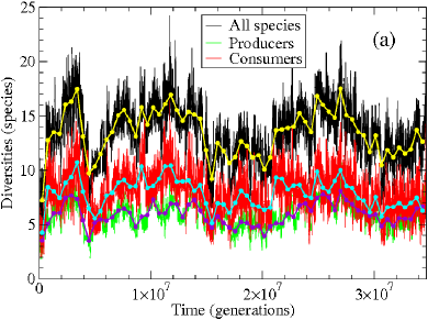
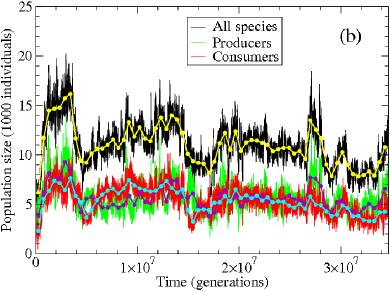
Figure 1: (Color online.) Time series for the Shannon-Wiener diversity index (a) and the population sizes (b). The jagged curves in the background show data sampled every 2048 generations to show the rapid fluctuations, while the curves in contrasting color/brightness in the foreground are running averages over 524 288 generations, emphasizing the slower fluctuations. The three sets of curves represent all species (black/light gray; black/yellow online), producer species (light gray/dark gray; green/violet online), and consumer species (medium gray/light gray; red/cyan online).

We collected time series of a number of quantities including several measures of diversity or species richness, as well as population sizes of producer and consumer species. Time series of diversities and population sizes for one representative run are shown in Fig. 1.

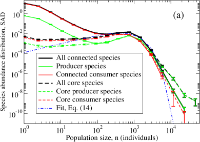
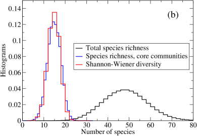
Figure 2: (Color online.) (a) Species abundance distributions (SADs), normalized to the number of species. Solid curves represent “full connected communities,” and dashed curves represent “core communities,” both extracted as described in the text. Both were sampled every 256 generations. The data were averaged over twelve independent simulation runs, and the error bars represent standard errors, based on the differences between runs. The dot-dashed curve is a fit to the curve describing all core species, using Eq. (14) with parameters $C=13.569$, $\mu=0.00210967$, and $\beta=1.89338$, interpolating between log-series and log-normal forms. (b) Histograms of the full-community species richness, the species richness of the core communities, and the Shannon-Wiener diversity for the sampled communities. The latter is seen to be an excellent approximation for the species richness of the core communities.

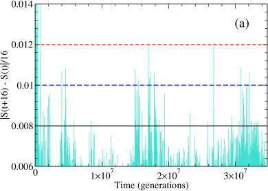
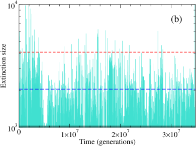
Figure 3: (Color online.) Time series for the same simulation run shown in Fig. 1, displaying quantities that measure the evolutionary activity: the magnitude of the logarithmic derivative of the Shannon-Wiener diversity index, $|dS/dt|$ (averaged over 16 generations) (a), and the size of extinctions per generation (b). The horizontal lines in each part indicate cutoff levels used to define quiet and active periods as discussed in Sec. IV.4.

In order to filter out noise from the small-population species that are mostly unsuccessful mutations, we use the diversity measure known in ecology as the exponential Shannon-Wiener index Krebs (1989). It is defined as the exponential function of the information-theoretical entropy of the population distributions, $D(t)=\exp\left[S\left(\{n_{I}(t)\}\right)\right]$, where

$$S\left(\{n_{I}(t)\}\right)=-\sum_{\{I|\rho_{I}(t)>0\}}\rho_{I}(t)\ln\rho_{I}(t)$$ (13)

with $\rho_{I}(t)=n_{I}(t)/N_{\rm tot}(t)$ for the case of the curves labeled “All species” in Fig. 1. For the producers or consumers, the sums and normalization constant include only the appropriate species. The utility of the Shannon-Wiener index is illustrated by the data presented in Fig. 2. In Fig. 2(a) we show two versions of the Species Abundance Distribution (SAD) for the model. This is one of the tools most widely used in ecology to describe the distribution of the number of species over population sizes Hughes (1986). The SADs shown as full lines in the figure represent full communities, from which we have only removed any consumer species that are not connected to the external resource through an unbroken chain of nonzero interactions. These we term “full connected communities” (”full communities” for short). (The removal of disconnected consumer species actually has a numerically insignificant effect on the SADs.) The SADs for the full communities are dominated by a large number of species with very small populations, which to a large extent represent unsuccessful mutants. This was explicitly shown by extracting “core communities” in the following way. Communities were sampled every 256 generations, and species with population sizes below eight were excluded. It was then checked whether each included species also existed with at least this minimum population 256 generations ago, and if this was not the case, the species was removed from the community as unstable. The fixed-point populations for the community of remaining species were then calculated according to Eq. (5), species with negative fixed-point populations (unfeasible species) were removed, and the fixed-point calculation was repeated until all species remaining in the community had positive populations. The SAD was then calculated for each of these feasible core communities and averaged over all communities in the twelve independent simulation runs. This procedure removes most of the low-population species, as shown by the dashed curves in Fig. 2(a). The core-community SAD appears to be intermediate between Fisher’s log-series distribution Hughes (1986); Fisher et al. (1943) and Preston’s log-normal distribution Hughes (1986); Preston (1948). It can be semiquantitatively approximated by fitting the constants $C$, $\mu$, and $\beta$ in the function Pigolotti et al. (2004)

$$p(n)=C\mu^{\beta}n^{\beta-1}e^{-\mu n}/\Gamma(\beta)\;,$$ (14)

which interpolates between these two limiting forms. The fit is shown by the dash-dotted curve in the figure. Additional evidence for the agreement between the Shannon-Wiener diversity index and the species richness of the core communities is shown in Fig. 2(b), where histograms of the two are in excellent agreement and both show a narrow peak near fifteen species (mean values of 15.7 and 15.3 species, respectively), while the raw species richness yields a wide distribution with a mean of 49.3 species. All three distributions are very well fit by gaussians and are much more symmetric than diversity distributions arising from Rossberg et al.’s speciation model of food webs Rossberg et al. (2006).

Time series of additional quantities that indicate the level of evolutionary activity are shown in Fig. 3 for the same simulation run as in Fig. 1. These are the magnitude of the logarithmic derivative of the Shannon-Wiener diversity index (Fig. 3(a)), and the size of extinctions per generation (Fig. 3(b)). The latter is defined as the sum of the maximum population sizes reached by the species that go extinct in each generation.

The properties of the fluctuations in the time series were analyzed with several methods, including power spectral densities (PSD), lifetimes of individual species, and the durations of quiet and active periods during the evolution. The results of each are reported in the following subsections.

IV.2 Power spectral densities

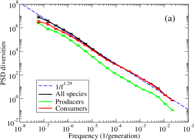
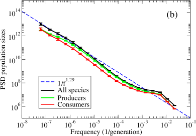
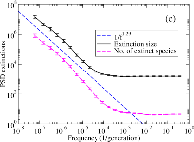
Figure 4: (Color online.) PSDs for the Shannon-Wiener diversities (a), population sizes (b), and the extinction sizes and number of species going extinct per generation (c), all averaged over twelve independent runs of $2^{25}$ generations. The error bars are standard errors, estimated from the variations between the individual runs. The dashed straight line with slope $-1.29$ in (a) is a weighted fit to the PSD for the overall diversity over the whole frequency range. The dashed lines in (b) and (c) are guides to the eye with the same slope.

PSDs of the diversity and population-size fluctuations, averaged over the twelve independent simulation runs, are shown in Fig. 4, both for the total population and for the producers and consumers separately. The spectra indicate $1/f$ like noise over more than five decades in time. A weighted fit to the PSD for the overall diversity in Fig. 4(a) yields a power law $f^{-\alpha}$ with $\alpha\approx 1.29\pm 0.01$. This power is also seen to fit reasonably well, both with the data for the diversities of producers and consumers over the whole frequency range in Fig. 4(a), and with the PSDs of all three population measures at low frequencies in Fig. 4(b), as well as for the extinction measures at low frequencies in Fig. 4(c). This suggests that the long-time fluctuations in the diversity, as well as in the population sizes and the extinction measures, obey the same power law on long timescales. On short timescales the PSDs for the population sizes have a more complicated structure, possibly indicating overdamped oscillations on a scale of a few hundred generations. The extinction measures show a wide region of white noise for high frequencies, due to the frequent extinction of unsuccessful mutants. However, the behaviors for low frequencies appear consistent with the diversities and the population sizes.

IV.3 Species lifetimes

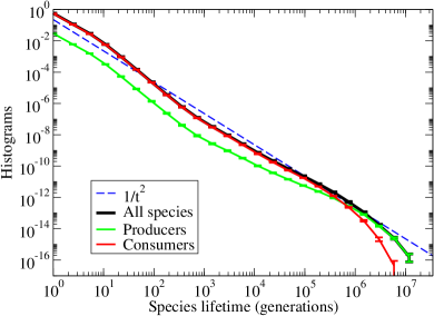
Figure 5: (Color online.) Histograms for the lifetimes of individual species. The dashed, straight line is a guide to the eye, corresponding to a $t^{-2}$ power law. Data averaged over 12 independent simulation runs.

The statistics of the lifetimes of individual species are characteristic of the evolution process. The species lifetime is defined as the time from a particular species enters the community, till it goes extinct (i.e., its first return time to zero population size). Histograms showing the distributions of species lifetimes, for all species as well as for producers and consumers separately, are shown in Fig. 5. Although there are some undulations in these curves, they remain close to a power law $t^{-\tau_{1}}$ with exponent $\tau_{1}\approx 2$ over more than six decades in time, which is the maximum we could expect with the length of our simulations.

The $t^{-2}$ dependence of the lifetime distributions is quite universal. It is found, e.g., in our previous studies of the mutualistic model Sevim and Rikvold (2005); Rikvold (2005, a), and it is in general characteristic of stochastic branching processes Pigolotti et al. (2005).

Lifetime distributions for marine genera that are compatible with a power-law exponent in the range $-1.5$ to $-2.5$ have been obtained from the fossil record Newman and Sibani (1999); Newman and Palmer (2003); Bornholdt et al. . However, the possible power-law behavior in the fossil record is only observed over about one decade in time – between 10 and 100 million years – and other fitting functions, such as exponential or log-normal, are also possible. Nevertheless, it is reasonable to conclude that the numerical results obtained from complex, interacting evolution models that extend over a large range of time scales support interpretations of the fossil lifetime evidence in terms of nontrivial power laws.

IV.4 Quiet and active periods

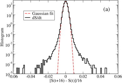
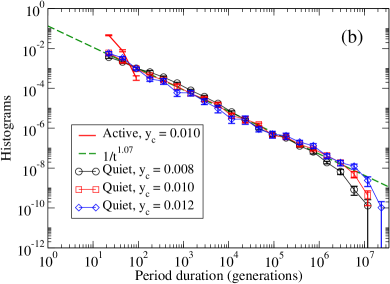
Figure 6: (a) Histogram of the logarithmic derivative of the overall diversity, $dS/dt$. The data were averaged over 16 generations for each run and then over 12 independent runs. The dashed curve is a gaussian fit. The time series of the magnitude of this quantity for one particular simulation run is shown in Fig. 3(a). (b) Histograms for the durations of active and quiet periods for various values of the cutoff $y_{c}$ for $|dS/dt|$, averaged over 12 independent runs. The dashed, straight line with slope $-1.07$ is a weighted fit to the histogram for the quiet periods for $y_{c}=0.010$ between 10 and $10^{6}$ generations. The steep histogram curve with only three data points between 10 and 100 generations corresponds to the active periods, which are always very short.

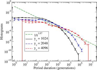
Figure 7: Histograms of the durations of quiet periods, obtained from the time series of extinction sizes, an example of which is shown in Fig. 3(b). Data averaged over 12 independent simulation runs. The straight, dashed line with slope $-1.07$ is a guide to the eye, based on the fit to the QSS duration distribution based on $|dS/dt|$, shown in Fig. 6(b).

From the time series shown in Figs. 1 and 3 one sees that periods of moderate fluctuations are punctuated by periods of high activity. The communities corresponding to the lower fluctuation intensities are known as quasi-steady states (QSS). (In the literature on the tangled-nature model Christensen et al. (2002); Hall et al. (2002); di Collobiano et al. (2003) the QSS are referred to as quasi evolutionarily steady strategies, or q-ESS.) The cores of these communities correspond to the fixed-point communities of the mutation-free system Rikvold and Zia (2003); Zia and Rikvold (2004), as discussed in Sec. IV.1. One measure of the degree of activity is the time derivative of the entropy or, equivalently, the logarithmic derivative of the total Shannon-Wiener diversity. Its magnitude is shown as a time series in Fig. 3(a), and a histogram is shown in Fig. 6(a). While the central part of the distribution is well approximated by a gaussian, the heavier wings appear to be exponential or even power-law. Quiet and active periods were defined as contiguous periods during which $|dS/dt|$ stayed below or above a cutoff $y_{c}$, respectively. Octave-binned histograms for the probability distributions of the durations of quiet and active periods are shown in Fig. 6(b) for various cutoffs. For the quiet periods a power law is seen with exponent near $-1$ (a weighted fit between 10 and $10^{6}$ generations gives $t^{-\tau}$ with $\tau\approx 1.07\pm 0.01$) and a long-time cutoff that increases with increasing $y_{c}$. The active periods for all values of $y_{c}$ are very brief in comparison. (Their histogram for $y_{c}=0.010$ is the steep curve with only three data points between 10 and 100 generations in Fig. 6(b).) As a consequence, the system spends most of its time in QSS communities – a situation consistent on the community level with Eldredge and Gould’s concept of punctuated equilibria Eldredge and Gould (1972); Gould and Eldredge (1977, 1993).

Durations of quiet periods could also be obtained from the time series of extinction sizes in Fig. 3(b). Due to the white noise at short timescales, which was also apparent in the PSDs in Fig. 4(c), the power-law behavior is limited to a window of longer times between about 1000 generations and the strongly cutoff-dependent long-time decay. As a result, this quantity does not provide as clear a quiet-period distribution as the entropy derivative. We therefore did not perform any independent fit to obtain a power-law exponent for the QSS durations measured this way. See Fig. 7. The decay with time is qualitatively consistent with that observed in Fig. 6(b) for the QSS duration distributions based on $|dS/dt|$.

It is quite remarkable that the exponent for the QSS durations is significantly different from the one for the species lifetimes, which is close to 2. This is particularly so because the two exponents appear to be approximately the same (both near 2) for the mutualistic version of the model Sevim and Rikvold (2005); Rikvold (2005, a). We believe that the explanation lies in the structure of the QSS communities generated by the present evolution process, which take the form of simple food webs. These are studied in Sec. IV.5 below.

IV.5 QSS community structure and stability

IV.5.1 General considerations

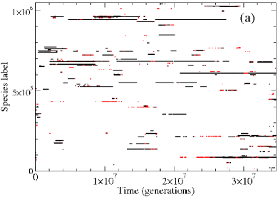
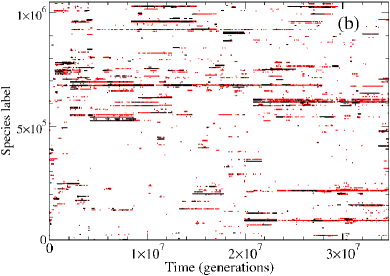
Figure 8: (Color online.) Major populated species shown vs time for the same simulation run shown in Figs. 1 and 3. The horizontal lines correspond to the species label, and the grayscale (color online) to the population size. Black: $n_{I}>1000$. Gray (red online): $n_{I}\in[101,1000]$. (a): Producers. (b): Consumers.

The evolution process in the present model generates dynamic communities, in which species emerge, exist for a shorter or longer time, and eventually go extinct. The emergence and extinction of a major species are quite fast processes on the evolutionary timescale, and so the vast majority of randomly selected communities are QSS communities. This is confirmed by the short durations of evolutionarily active periods, shown by the corresponding histogram in Fig. 6(b). Diagrams of the population sizes of major producer and consumer species as functions of time in a particular simulation run are shown in Figs. 8(a) and (b), respectively. In these figures a horizontal line represents a species. The beginning of the line represents the emergence of the species, and the end represents its extinction. The population size is represented by the color. We see that some species persist for tens of millions of generations, while others are so short-lived as to hardly be visible on the scale of these figures. This is consistent with the power-law behavior of the species-lifetime distribution (see Fig. 5). We also see that producer species appear to emerge and go extinct relatively independently of each other, while there is a significant correlation between the producer and consumer species. This correlation indicates that extinction of a producer species is likely to trigger a (limited) cascade of consumer extinctions. Conversely, a new producer species is likely to quickly acquire a group of consumer species. The structure of the plots in Fig. 8 contrasts with that of similar plots for the mutualistic model of Ref. Rikvold and Zia (2003) (see Fig. 2 of that paper), in which species tend to emerge as well as go extinct together. We believe this is the reason for the difference between the exponents for the species lifetimes and the durations of QSS communities in this model: the overall community is relatively resilient toward losing or gaining a single species Drossel et al. (2001); Dunne et al. (2002a); Dunne et al. (2004); Quince et al. (2005a). As a community it is more long-lived than the individual species, leading to the smaller value for the exponent of the distribution for the QSS durations (compare Figs. 5 and 6(b)). (A similar relationship has been noted between the lifetimes of orders and their constituent genera in the fossil record Bornholdt et al. .)

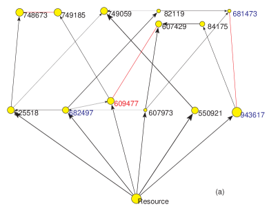
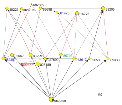
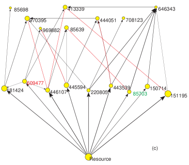
Figure 9: (Color online.) Food webs representing QSS core communities for the simulation shown in Figs. 1, 3, and 8 at times near $22\times 10^{6}$ generations (a), near $27\times 10^{6}$ generations (b), and at the end of the simulation near $35\times 10^{6}$ generations (c). The core communities were identified as described in Sec. IV.1. The thickness and head size of the arrows correspond to the magnitude of $M_{IJ}$, and the area of the circles to the stationary population size, as calculated analytically from Eq. (5). Light gray (red online) lines connect nearest neighbors in genotype space. Labels in red mark species that persist from the first to the last snapshot, (a) to (c), while blue labels mark species that persist from (a) to (b), and and green labels mark species that persist from (b) to (c). Black labels indicate species that are unique to the particular community.

Three representative QSS core communities from the same simulation run shown in Figs. 1, 3, and 8 are shown in Fig. 9. These are consecutive core communities near $22\times 10^{6}$, $27\times 10^{6}$, and $34\times 10^{6}$ generations, respectively, and they are all stable by the eigenvalue criterion discussed in Sec. III.2. The communities take the form of simple food webs with two trophic levels above the resource node. Communities with three trophic levels are also occasionally observed. The different branches of the webs are relatively independent of each other, and many consumer species have more than one prey. (See further quantitative discussion in Sec. IV.5.2.) Both features contribute to the resilience against mass extinctions discussed above.

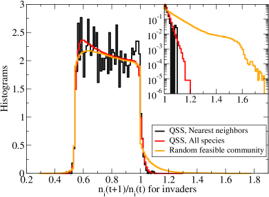
Figure 10: (Color online.) Histograms of the multiplication ratio, $n_{i}(t+1)/n_{i}(t)$ (exponential of the invasion fitness, Eq. (12)) for low-density invaders. Each curve is averaged over 14 different core communities. Black: nearest neighbors in genotype space against stable QSS communities. Dark gray (red online): All species not in the community against stable QSS communities. Light gray (orange online): All species not in the community against random feasible communities. Inset: The part of the distributions for potentially successful invaders, $n_{i}(t+1)/n_{i}(t)>1$, with the $y$-axis on logarithmic scale. The tails appear nearly exponential.

The relative stability of evolved QSS core communities with respect to invasion by mutants is illustrated in Fig. 10. The results are averaged over 14 QSS core communities – the three shown in Fig. 9 plus the final communities of the eleven other simulation runs. This figure shows the multiplication ratio of a small population of invaders (the exponential function of the invasion fitness), given by Eq. (12). Only about 2.3% of species outside the communities have multiplication ratios larger than unity, and most of these lie between 1.0 and 1.1. This percentage does not seem to depend significantly on the Hamming distance of the invader from the community. We note that the species that are removed from the community during extraction of the core community are among these low invasion fitness species. This is a further indication that the difference between core and full communities is mostly made up by unsuccessful mutants.

We also tested if the evolved core communities are more resilient toward invasion than randomly constructed feasible communities. Such communities are more difficult to construct in this model, than in the mutualistic model Rikvold and Zia (2003). To have the same level of statistics as for the QSS communities, we produced 14 such communities in the following way. We started a run with a random sample of 200 species, each with $n_{I}=10$, and evolved the community for 1024 generations without mutations. We then tested the remaining community for feasibility and removed species with a negative stationary population according to Eq. (5). The resulting feasible communities had much smaller diversities than the evolved QSS communities – an average of only 3.6 species per community. These communities had a significantly larger percentage of potential invaders – about 4%, with a maximum multiplication ratio near 1.7 (see inset in Fig. 10). While there thus is a clear difference between the stability against invaders of QSS communities and random feasible communities, the difference is not as large as it is for the mutualistic model of Ref. Rikvold and Zia (2003). (See Fig. 3 of that paper.)

IV.5.2 Detailed community structure and comparison with real food webs

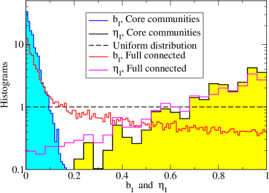
Figure 11: (Color online.) Log-linear plot of histograms of the birth cost $b_{I}$ (left) and producer coupling to the external resource, $\eta_{I}$ (right), for members of QSS core communities (shaded areas) and full communities (lines only). Both parameters are selected away from the uniform distributions of the full species pool (represented by the horizontal dashed line).

Next we turn to a detailed statistical description of the QSS core and full connected communities identified in Sec. IV.1. Since communities were extracted every 256 generations from twelve independent runs of $2^{25}$ generations each, data were averaged over $131\,072\times 12$ communities of each type. However, due to the long-time correlations in the evolution process, many of the communities from the same run are identical or similar. This sampling method thus ensures that the statistics for both communities and individual species are weighted according to their longevities. First we consider the properties of individual species, and next we turn to the collective properties of the corresponding food webs and a comparison with data for real food webs.

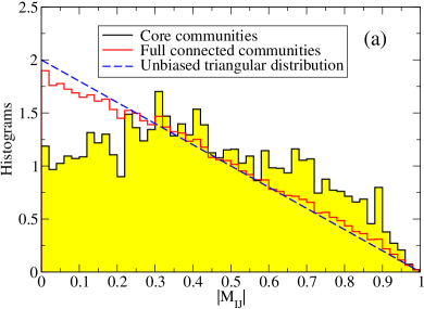
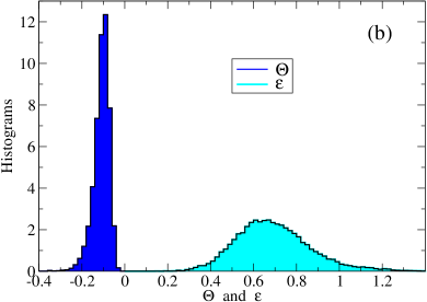
Figure 12: (Color online.) Histograms of community-level parameters. (a) The interspecies interaction strengths, $|M_{IJ}|$, for QSS core and full communities. (b) The effective interaction strength $\Theta$ (left) and resource coupling $\mathcal{E}$ (right) for QSS core communities, defined in Eq. (7).

The individual species are characterized by the birth cost $b_{I}$, the self interaction $M_{II}$, and for producers by the resource coupling $\eta_{I}$. In the total pool of potential species these are uniformly distributed on $(0,+1]$, $[-1,0)$, and $(0,+1]$, respectively. Not surprisingly, the most prevalent species in the core communities turn out to be the most “individually fit” ones in the sense that they have low birth cost and, for producers, relatively strong coupling to the external resource. The resulting probability densities for $b_{I}$ and $\eta_{I}$ are shown in Fig. 11. The selection for low birth cost is very strong for members of the core communities, and less so when the full communities are considered. This is further indication that the species that are ignored when extracting the core communities have higher $b_{I}$, and thus overall are less individually fit, than the core species. On the other hand, the moderate selection for strong coupling to the external resource (large $\eta_{I}$) is approximately equal for producers in both types of communities. In contrast, the self interactions appear to be evolutionarily neutral, and their probability density remains approximately uniform for the members of both core and full communities (not shown).

The first community-level quantities we consider are the nonzero interspecies interaction strengths, $|M_{IJ}|$. Histograms for these, based on the same sampling and averaging as previous results, are shown in Fig. 12(a). The distribution for the core communities is significantly skewed toward strong interactions, compared to the triangular distribution characteristic of the total species pool, which is shown as a dashed line. The bias is much weaker when all members of the full communities are considered. (See Appendix A for a discussion of the unbiased distribution.)

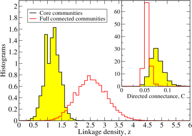
Figure 13: (Color online.) Histograms for the linkage density, $z=L/S$ (main part) and the directed connectance, $C=L/S^{2}$ (inset), for the model communities.

The biased distribution of interaction strengths combines with the strongly skewed distributions of $b_{I}$ and $\eta_{I}$ to produce values of the effective interaction strength $\Theta$ and effective resource coupling $\mathcal{E}$ for the core communities (defined in Eq. (7)) that are in excellent agreement with the expectations expressed in Sec. III.1. As shown in Fig. 12(b), $\Theta$ is narrowly distributed closely below 0 ($\overline{\Theta}=-0.10$), while $\mathcal{E}$ has a broader distribution over positive values with mean $\overline{\mathcal{E}}=0.71$. These averages are in excellent agreement with those obtained from the final communities of the twelve runs, obtained in Sec. IV.1.

Next we consider several quantities from network theory that can be compared with data from real food webs. These include the directed connectance, $C=L/S^{2}$, where $L$ is the number of links (i.e., the number of nonzero $M_{IJ}$, $M_{JI}$ pairs) and $S$ is the diversity (here defined as the species richness), the linkage density, $z=L/S=CS$, the probability distributions of a species’ number of prey species (its generality or indegree), number of predator species (its vulnerability or outdegree), and their sum (its total degree) Rossberg et al. (2006).

For comparison with the simulated food webs generated by our evolutionary model, we use data for seventeen empirical webs, including both aquatic and terrestrial communities. These data sets were kindly provided to us by J. A. Dunne. Tabular overviews of the parameters characterizing these communities are available in the literature Dunne et al. (2002a, b); Dunne et al. (2004); Quince et al. (2005b). For all the empirical webs we defined the diversity as the species richness $S$ in terms of trophic species. These are obtained by lumping together all taxa that share all their predators and prey Williams and Martinez (2000); Dunne et al. (2002b). Like the simulated communities analyzed, the empirical webs contain no disconnected species or subwebs Dunne et al. (2002b). The included empirical food webs are: Coachella Valley Polis (1991), El Verde Rainforest Wai (1996), Scotch Broom Memmott et al. (2000), St. Martin Island Goldwasser and Roughgarden (1993), and U.K. Grassland Martinez et al. (1999) (terrestrial); Bridge Brook Lake Havens (1992), Little Rock Lake Martinez (1991), and Skipwith Pond Warren (1989) (lake or pond); Canton Creek Townsend et al. (1998) and Stony Stream Townsend et al. (1998) (stream); Chesapeake Bay Baird and Ulanowicz (1989), St. Mark’s Estuary Christian and Luczkovich (1999), Ythan Estuary Hall and Raffaelli (1991), and Ythan Estuary with parasites Huxham et al. (1996), (estuaries); Benguela Yodzis (1998), Caribbean Reef – small Opitz (1996), and North-eastern U.S. continental shelf Link (2002) (marine).

As discussed above, the food webs produced by the evolutionary process in this model are relatively small, with average diversity $\overline{S}\approx 15$ for the QSS core communities and approximately 50 for the full communities. As seen in Fig. 13, the directed connectance $C$ is somewhat smaller ($\overline{C}\approx 0.08$ for core and $\overline{C}\approx 0.06$ for full communities) than the input connectance, $c=0.1$. However, this is partly because it is calculated in the conventional way as $L/S^{2}$ Rossberg et al. (2006), rather than as $L/S(S-1)$. The average linkage density is also quite small ($\overline{z}=1.17$ for core and $\overline{z}=2.58$ for full communities) compared to most of the real food webs that have been documented. For comparison, the seventeen documented food webs have $\overline{S}\approx 69$ with a range from 25 to 155, $\overline{C}\approx 0.13$ with a range from 0.03 to 0.32, and $\overline{z}\approx 6.9$ with a range from 1.6 to 17.8. However, Williams and Martinez’ niche model for food-web structure Williams and Martinez (2000) leads to a scaling hypothesis for the degree distributions (exact for the niche-model prey distribution and approximate for the predator distribution) Camacho et al. (2002a, b); Stouffer et al. (2005):

$$2zp(k)=\tilde{p}_{k}(k/2z)\;,$$ (15)

where $k$ can be either the generality, the vulnerability, or the total degree (with different scaling functions $\tilde{p}$ for each). As a consequence, cumulative degree distributions can also be rescaled by simply dividing the argument by $2z$. Using this niche-model result as a general scaling hypothesis Rossberg et al. (2006), we can compare the degree distributions for the communities generated by our model with scaled data for the seventeen real food webs.

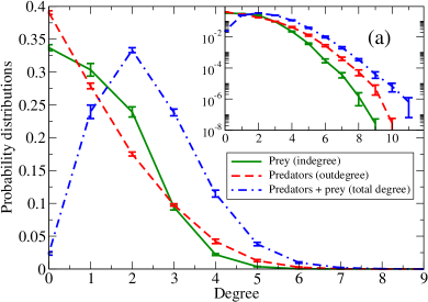
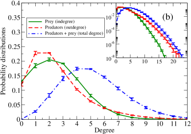
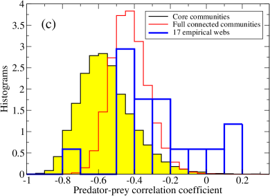
Figure 14: (Color online.) (a) Unscaled degree distributions for the QSS core communities, showing number of prey (solid), number of predators (dashed), and total degree (dot-dashed). The distributions were individually normalized for each community, and then averaged over all communities. The error bars are standard errors, based on the spread between the twelve simulation runs. Average linkage density is $\overline{z}=1.17$. The inset on log-linear scale shows that these distributions decay at least exponentially with increasing argument. (b) Same as (a), for the full communities. Average linkage density is $\overline{z}=2.58$. (c) Histograms over individual sampled communities of the correlation coefficient between a species’ numbers of predators and prey. Black filled with light gray (yellow online): QSS core communities. Medium gray (red online): full, connected communities. Dark gray (blue online) with drop lines: empirical data for seventeen natural food webs.

The degree distributions for the model, individually normalized for each community, and then averaged over all communities, are shown in unscaled form in Fig. 14(a) and (b). As seen from the insets, all three distributions (prey, predators, and total degree) decay at least exponentially for large argument. This property is shared by most real food webs Dunne et al. (2002b) and models Camacho et al. (2002a, b); Rossberg et al. (2006); Sevim and Rikvold (2006) and indicates that food webs in general are not scale-free networks. The behavior for $k<2z$ is more model and system dependent.

Histograms for the correlations between a species’ generality and vulnerability are shown in Fig. 14(c), together with data for the seventeen real food webs. The average correlation coefficients are $-0.53$ for core communities and $-0.40$ for full communities, more negative than, but not inconsistent with, the real food-web average of $-0.23$.

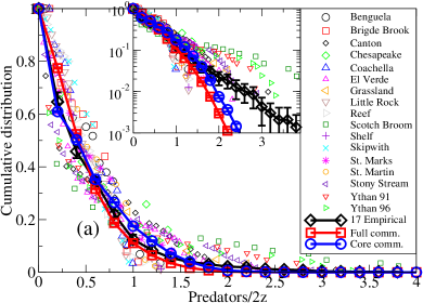
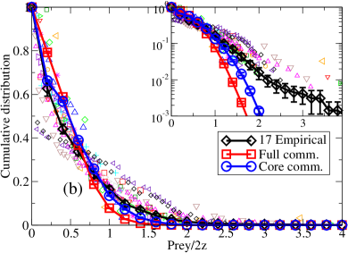
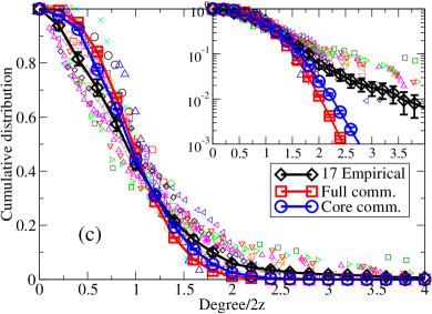
Figure 15: (Color online.) Scaled, cumulative degree distributions for the model, compared with results for the seventeen empirical food webs. Data for individual, real food webs are shown in the background as isolated data points. Average data for the simulated and real webs are shown as data points with error bars indicating standard error, connected by heavy lines. Dark gray with circles (blue online): simulated core communities. Medium gray with squares (red online): simulated full communities. Black with diamonds: empirical communities. Details of the averaging are discussed in the text. (a) Number of predators (vulnerability, or outdegree). (b) Number of prey (generality, or indegree). (c) Number of predators plus prey (total degree).

Due to the relatively small size of the empirical food webs, it is difficult to extract information from scaled probability densities, which will include empty bins unless a very large bin size is chosen. This problem is avoided by instead studying the cumulative distribution, $P(x)={\rm Prob}\left[k/(2z)>x\right]$ Dunne et al. (2002b). These are shown in Fig. 15 for the seventeen empirical webs, together with averaged results for the empirical webs and the model. The averaged curves were generated by first scaling the degrees (predators, prey, and total) for each web by the value of $2z$ for that particular web, binning the results in bins of width 0.2, and normalizing the binned histogram by the species richness $S$ of that same web. The individually scaled, binned, and normalized histograms were then averaged over all webs (seventeen for the empirical webs and $131\,072\times 12$ for the model webs) and finally integrated to produce the average scaled cumulative distributions. For the model, results are shown both for the full and core communities.

Despite their smaller average diversity and linkage density, the scaled cumulative degree distributions for both types of model communities, which are shown in Fig. 15, fall well within the range of the empirical data. For scaled degrees below about 1.5, the averaged distributions for the core communities are in quite reasonable agreement with those for the empirical food webs. The largest deviations are for total degree (Fig. 15(c)) at small values of the scaled argument. This is possibly due to the significantly stronger negative correlations between the numbers of predators and prey (vulnerability and generality) for species in the model communities, compared to the empirical ones. (See Fig. 14(c).) For scaled degrees above approximately 1.5, the averages for the empirical webs are significantly above those for the model webs and appear approximately exponential in the tail (see insets in Fig. 15). We note, however, that this behavior in the averages is caused by a small number of webs; the remaining empirical webs have no species of such highly above-average degrees. Overall, the scaled, cumulative distributions for the present model agree with the empirical data to about the same degree as the niche model Stouffer et al. (2005) and the speciation model of Rossberg et al. Rossberg et al. (2005, 2006). However, it must be admitted that much potentially valuable detail about the food-web structure is lost in calculating the cumulative distributions.

A measure of the hierarchical structure of a food web is given by the proportions of basal species (species with no prey, supported only by the external resource), intermediate species (that have both prey and predators) and top species (that have no predators). As seen from the histograms in Fig. 16, there are wide variations from community to community for each class of species. The high proportion $I$ of intermediate species seen for the full communities in Fig. 16(b) ($I=0.76$) is consistent with most of the real food webs analyzed, including Caribbean Reef ($I=0.94$), U.S. Shelf ($I=0.94$), Benguela ($I=0.93$), Scotch Broom ($I=0.92$), Skipwith Pond ($I=0.92$), Coachella Valley ($I=0.90$), Little Rock Lake ($I=0.86$), El Verde Rainforest ($I=0.69$), St. Marks Seagrass ($I=0.69$), St. Martin Island ($I=0.69$), and Bridge Brook Lake ($I=0.68$), as well as simulations of the Web World model Quince et al. (2005b) and mean-field analysis of a Lotka-Volterra predator-prey model with evolution and competition Lässig et al. (2001). The core communities, on the other hand, have their member species much more evenly distributed among the three classes, as shown in Fig. 16(a). Real food webs with more even distributions are Canton Creek ($B=0.53$, $I=0.22$, $T=0.25$), Stony Stream ($B=0.56$, $I=0.27$, $T=0.17$), and Chesapeake Bay ($B=0.16$, $I=0.52$, $T=0.32$). Thus, at least in this model, and somewhat counterintuitively, on average the intermediate species are both the least stable and the most numerous.

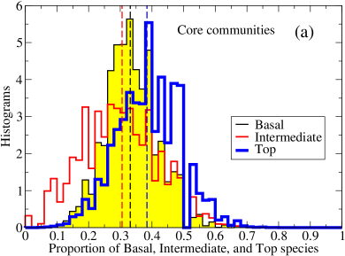
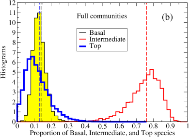
Figure 16: (Color online.) Histograms for the proportions of basal, intermediate, and top species. The vertical, dashed lines in matching grayscale (color) represent the mean proportion for each class. (a) Core communities. Mean proportions: 0.33 for basal, 0.31 for intermediate, and 0.38 for top species. (b) Full communities. Mean proportions: 0.14 for basal, 0.76 for intermediate, and 0.13 for top species.

We conclude these comparisons of the structures of food webs evolving in the present model to data for real food webs with some words of caution. The model was primarily developed to study the long-time temporal fluctuations in diversity and population size, and it was in no way tuned to produce realistic community structures except insofar as they are generally food-web like. This community structure does, however have profound effects on the dynamics, as it is responsible for the difference between the power-law exponents for the lifetimes of species and communities in this predator-prey model. One should also note that, while the lack of correlations between the properties of closely related species was shown to have little effect on the long-time dynamics Sevim and Rikvold (2005), we have not considered whether such correlations might affect the detailed community structure. Most likely they would, at least to some degree. In addition, the growth of real food webs involve a number of mechanisms, besides just evolution and local population dynamics. Most notably, immigration plays an important role in the occurrence of new members of a spatially localized community. However, due to the large differences between parent species and mutants in the current model, our evolution mechanism may also been seen as covering immigration.

We also note that the simulated communities have significantly smaller diversities, connectances, linkage densities, and population sizes than the real communities, so that our comparisons had to rely heavily on scaling arguments. It would therefore be desirable in future studies to increase the connectance, number of potential species, and resource size to bring the results closer to the realistic range.

V Summary and Conclusions

In this paper we have studied in detail an individual-based predator-prey model of biological coevolution, based on the simplified version of the tangled-nature model Christensen et al. (2002); Hall et al. (2002); di Collobiano et al. (2003) that was introduced in Ref. Rikvold and Zia (2003). Selection is provided by a population-dynamics model in which the reproduction probability of an individual of a particular species depends nonlinearly on the amount of external resources and on the population densities of all other species resident in the community. New species appear in the community through point mutations in a genome consisting of a string of $L$ bits.

In the mutation-free limit, the mean fixed-point population sizes and stability properties of any $\mathcal{N}$-species community can be obtained exactly by linear stability analysis. While the universal competition effect that enables this analytical treatment is not very realistic, the exact solutions make the model ideal as a benchmark for more realistic, but also more complicated, models. A preliminary discussion of two more realistic models is found in Ref. Rikvold (b).

In the simulations presented here, we used $L=20$ for a total of $2^{20}=1\,048\,576$ potential species. In order to study the statistically stationary properties of the model, we performed long kinetic Monte Carlo simulations over $2^{25}=33\,554\,432$ generations. By studying the stationary fluctuations we hope in the future to gain an understanding of the the system’s sensitivity to external perturbations in a way analogous to the fluctuation-dissipation relations of equilibrium statistical mechanics Sato et al. (2003).

Qualitatively, many of the statistical properties of this model are similar to those of the related, mutualistic model studied in Refs. Rikvold and Zia (2003); Zia and Rikvold (2004); Sevim and Rikvold (2005). These include approximate $1/f$ noise in power spectra (PSDs) of diversity and population sizes ($f^{-\alpha}$ with $\alpha\approx 1.29$), and power-law distributions for the lifetimes of individual species, as well as of the durations of evolutionarily quiet periods, corresponding to QSS communities. However, in contrast to the mutualistic model, the power-law exponents for the species lifetimes and QSS durations are different: $t^{-\tau_{1}}$ with $\tau_{1}\approx 2$ for the former (consistent with a stochastic branching process Pigolotti et al. (2005)) and $t^{-\tau}$ with $\tau\approx-1.07$ for the latter. In Ref. Rikvold (2005) it was speculated that the exponent values $\alpha=1$, $\tau_{1}=2$, and $\tau=1$ are consistent with predictions for a zero-dimensional extremal-dynamics model Paczuski et al. (1996); Dorogovtsev et al. (2000). However, this speculation is not consistent with the presumably more accurate estimate for $\alpha$ presented here, and it seems advisable to be rather skeptical about any mapping of the current model onto a simple statistical-mechanical extremal-dynamics model.

It is probably more fruitful to consider why $\tau_{1}$ and $\tau$ are different for the current predator-prey model, while they coincide for the corresponding mutualistic model. Here we believe the answer lies in the different community structures in the two models. While communities in the mutualistic model are tightly knit with all positive interactions (see Fig. 10 of Ref. Rikvold (a)), the communities in the present predator-prey model take the form of simple food webs, which are much more resilient toward the loss of a single or a few species. In this sense, this predator-prey model is in much better agreement with real food webs than the mutualistic model Drossel et al. (2001); Dunne et al. (2002a); Dunne et al. (2004); Quince et al. (2005a).

Our comparisons of the structure of the communities generated by our model with real food webs show both similarities and differences. A difficulty with such comparisons is the large differences in diversity and linkage density between the simulated and real webs, which necessitated heavy use of scaling arguments in the quantitative comparisons. For comparison of detailed community properties, simulations of models with higher diversity and connectance are therefore desirable in the future. Nevertheless, our model presents a synthesis of long-term evolutionary dynamics and food-web like communities within an individual-based framework of integrated population dynamics and evolution, that should provide a sound basis for more refined models in the future.

Appendix A Matrix Elements for Larger Genomes

Here we describe an improved version of the method introduced by Hall et al. Hall et al. (2002); Christensen et al. (2002) to produce pseudorandom matrix elements $M_{IJ}$ for values of $L$ that are too large for the full $2^{L}\times 2^{L}$ matrix $\bf M$ to fit into computer memory. This method permits the matrix elements for a given community to be generated and retained only as needed. We first present Hall et al.’s method, point out some problematic features, and then present our modifications.

Let ${\bf S}(I)$ be the string of binary digits corresponding to the decimal species label $I$. This bit string has length $L$, so there are $2^{L}$ different strings. To generate the matrix element $M_{IJ}$, one first generates a new string of the same length, ${\bf S}(I,J)={\bf S}(I)\,{\sf XOR}\,{\bf S}(J)$, where ${\sf XOR}$ is the logical exclusive or operator. From this bit string is generated the corresponding new decimal index $K\left({\bf S}(I,J)\right)$. Next one creates two one-dimensional arrays, ${\tt X}$ and ${\tt Y}$, each of $2^{L}$ random numbers between $-1$ and $+1$. (For simplicity let the starting index for the arrays be zero.) Since ${\bf S}(I,J)$ is symmetric in $I$ and $J$, asymmetric pseudorandom matrix elements are generated as

$$M_{IJ}=\left[{\tt X}\left(K\left({\bf S}(I,J)\right)\right)+{\tt Y}\left(J\right)\right]/2\;.$$ (16)

(Hall et al. instead use the product of the two random numbers, which gives a pseudorandom number with a slightly different distribution.)

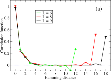
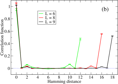
Figure 17: (Color online.) Normalized correlation functions for the matrix elements $M_{IJ}$ for the two schemes described in the text, each based on a single realization of $\bf M$ for $L=6$, 8, and 9. (a) The scheme described in Ref. Hall et al. (2002). (b) The modified scheme introduced here.

The problem with this method is that it produces strong correlations along the columns of $\bf M$ since the second of the two random numbers that produce $M_{IJ}$ is the same for all $I$ at the same $J$. In Fig. 17(a) we show the resulting correlation function for this scheme as a function of the Hamming distance between the pairs of bit strings involved in two different matrix elements. Regardless of $L$, significant correlations are seen for Hamming distances less than five. A discussion of how to calculate such correlation functions is found in Ref. Sevim and Rikvold (2005).

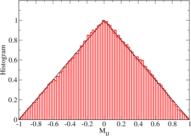
Figure 18: (Color online.) Histogram for the pseudorandom $M_{IJ}$ produced by the scheme introduced here for $L=9$, corresponding to 262 144 individual matrix elements. The straight, black lines represent the triangular shape of the theoretical distribution.

To reduce these correlations between matrix elements involving closely related genotypes, we here modify the scheme as follows. We extend array $\tt Y$ to a length of $3\times 2^{L}$ and define $M_{IJ}$ as

$$M_{IJ}=\left[{\tt X}\left(K\left({\bf S}(I,J)\right)\right)+{\tt Y}\left(K\left({\bf S}(I,J)\right)+2(J+1)\right)\right]/2\;.$$ (17)

The addition of $K\left({\bf S}(I,J)\right)$ in the index of $\tt Y$ ensures that the matrix element depends in an erratic fashion on both $I$ and $J$, while the term linear in $J$ ensures that $\bf M$ is not symmetric. The resulting correlation function is shown in Fig. 17(b). The correlations for elements involving closely related genotypes are strongly suppressed. The correlations for a Hamming distance of $2L$, which are present in both schemes, are of little practical significance. They are caused by the fact that the ${\sf XOR}$ operation is invariant under simultaneous bit reversal in both its arguments and could be removed by adding a linear function of $I$ in the argument of $\tt X$. The probability density for $M_{IJ}$ is triangular as expected from simple analytical arguments, and the whole interval from $-1$ to $+1$ is well sampled, even for relatively small $L$. This is shown in Fig. 18.

References

- Baake and Gabriel (2000) E. Baake and W. Gabriel, in Annual Reviews of Computational Physics VII, edited by D. Stauffer (World Scientific, Singapore, 2000), pp. 203–264.
- Drossel (2001) B. Drossel, Adv. Phys. 50, 209 (2001).
- Newman and Sibani (1999) M. E. J. Newman and P. Sibani, Proc. R. Soc. Lond. B 266, 1583 (1999).
- Newman and Palmer (2003) M. E. J. Newman and R. G. Palmer, Modeling Extinction (Oxford University Press, Oxford, 2003).
- (5) S. Bornholdt, K. Sneppen, and H. Westphal, e-print arXiv:q-bio.PE/0608033 (2006).
- Thompson (1998) J. N. Thompson, Trends Ecol. Evol. 13, 329 (1998).
- Thompson (1999) J. N. Thompson, Science 284, 2116 (1999).
- Drossel et al. (2001) B. Drossel, P. G. Higgs, and A. J. McKane, J. theor. Biol. 208, 91 (2001).
- Yoshida et al. (2003) T. Yoshida, L. E. Jones, S. P. Ellner, G. F. Fussmann, and N. G. Hairston, Nature 424, 303 (2003).
- Kocher (2004) T. D. Kocher, Nature Reviews. Genetics 5, 288 (2004).
- Crosby (1970) J. L. Crosby, Heredity 25, 253 (1970).
- Kauffman and Johnsen (1991) S. A. Kauffman and S. Johnsen, J. theor. Biol. 149, 467 (1991).
- Kauffman (1993) S. A. Kauffman, The origins of order. Self-organization and selection in evolution (Oxford University Press, Oxford, 1993).
- Caldarelli et al. (1998) G. Caldarelli, P. G. Higgs, and A. J. McKane, J. theor. Biol. 193, 345 (1998).
- Drossel et al. (2004) B. Drossel, A. McKane, and C. Quince, J. theor. Biol. 229, 539 (2004).
- Christensen et al. (2002) K. Christensen, S. A. di Collobiano, M. Hall, and H. J. Jensen, J. theor. Biol. 216, 73 (2002).
- Hall et al. (2002) M. Hall, K. Christensen, S. A. di Collobiano, and H. J. Jensen, Phys. Rev. E 66, 011904 (2002).
- di Collobiano et al. (2003) S. A. di Collobiano, K. Christensen, and H. J. Jensen, J. Phys. A 36, 883 (2003).
- Rikvold and Zia (2003) P. A. Rikvold and R. K. P. Zia, Phys. Rev. E 68, 031913 (2003).
- Zia and Rikvold (2004) R. K. P. Zia and P. A. Rikvold, J. Phys. A 37, 5135 (2004).
- Sevim and Rikvold (2005) V. Sevim and P. A. Rikvold, J. Phys. A 38, 9475 (2005).
- Chowdhury et al. (2003) D. Chowdhury, D. Stauffer, and A. Kunwar, Phys. Rev. Lett. 90, 068101 (2003).
- Chowdhury and Stauffer (2005) D. Chowdhury and D. Stauffer, J. Biosciences 30, 277 (2005).
- Gavrilets and Boake (1998) S. Gavrilets and C. R. B. Boake, Am. Nat. 152, 706 (1998).
- Gavrilets et al. (2000) S. Gavrilets, H. Li, and M. D. Vose, Evolution 54, 1126 (2000).
- Gavrilets and Vose (2005) S. Gavrilets and A. Vose, Proc. Natl. Acad. Sci. USA 102, 18040 (2005).
- Solé et al. (1996) R. V. Solé, J. Bascompte, and S. Manrubia, Proc. R. Soc. Lond. B 263, 1407 (1996).
- Rikvold (2005) P. A. Rikvold, in Noise in Complex Systems and Stochastic Dynamics III, edited by L. B. Kish, K. Lindenberg, and Z. Gingl (SPIE, The International Society for Optical Engineering, Bellingham, WA, 2005), pp. 148–155, e-print arXiv:q-bio.PE/0502046.
- Rikvold (a) P. A. Rikvold, submitted to J. Math. Biol. E-print: q-bio.PE/0508025.
- Sato et al. (2003) K. Sato, Y. Ito, T. Yomo, and K. Kaneko, Proc. Natl. Acad. Sci. USA 100, 14086 (2003).
- Eigen (1971) M. Eigen, Naturwissenschaften 58, 465 (1971).
- Eigen et al. (1988) M. Eigen, J. McCaskill, and P. Schuster, J. Phys. Chem. 92, 6881 (1988).
- Gavrilets (1999) S. Gavrilets, Proc. R. Soc. Lond. B 266, 817 (1999).
- Gavrilets (2004) S. Gavrilets, Fitness landscapes and the origin of species (Princeton University Press, Princeton and Oxford, 2004).
- Dunne et al. (2002a) J. Dunne, R. J. Williams, and N. D. Martinez, Ecol. Lett. 5, 558 (2002a).
- Garlaschelli (2004) D. Garlaschelli, Eur. Phys. J. B 38, 277 (2004).
- Verhulst (1838) P. F. Verhulst, Corres. Math. et Physique 10, 113 (1838).
- Murray (1989) J. D. Murray, Mathematical Biology (Springer-Verlag, Berlin, 1989).
- Roberts (1974) A. Roberts, Nature (London) 251, 607 (1974).
- Hardin (1960) G. Hardin, Science 131, 1292 (1960).
- Armstrong and McGehee (1980) R. A. Armstrong and R. McGehee, Am. Nat. 115, 151 (1980).
- den Boer (1986) P. J. den Boer, Trends Ecol. Evol. 1, 25 (1986).
- Hubbell (2001) S. P. Hubbell, The Unified Neutral Theory of Biodiversity and Biogeography (Princeton University Press, Princeton, 2001).
- Metz et al. (1992) J. A. J. Metz, R. M. Nisbet, and S. A. H. Geritz, Trends Ecol. Evol. 7, 198 (1992).
- Doebeli and Dieckmann (2000) M. Doebeli and U. Dieckmann, Am. Nat. 156, S77 (2000), and references therein.
- Stauffer and Aharony (1992) D. Stauffer and A. Aharony, Introduction to Percolation Theory. Second Edition. (Taylor & Francis, London, 1992).
- Krebs (1989) C. J. Krebs, Ecological Methodology (Harper & Row, New York, 1989), chap. 10.
- Hughes (1986) R. G. Hughes, Am. Nat. 128, 879 (1986).
- Fisher et al. (1943) R. A. Fisher, A. S. Corbet, and C. B. Williams, J. Animal Ecol. 12, 42 (1943).
- Preston (1948) F. W. Preston, Ecology 29, 254 (1948).
- Pigolotti et al. (2004) S. Pigolotti, A. Flammini, and A. Maritan, Phys. Rev. E 70, 011916 (2004).
- Rossberg et al. (2006) A. G. Rossberg, H. Matsuda, T. Amemiya, and K. Itoh, J. theor. Biol. 238, 401 (2006).
- Pigolotti et al. (2005) S. Pigolotti, A. Flammini, M. Marsili, and A. Maritan, Proc. Natl. Acad. Sci. USA 102, 15747 (2005).
- Eldredge and Gould (1972) N. Eldredge and S. J. Gould, in Models In Paleobiology, edited by T. J. M. Schopf (Freeman, Cooper, San Francisco, 1972), pp. 82–115.
- Gould and Eldredge (1977) S. J. Gould and N. Eldredge, Paleobiology 3, 115 (1977).
- Gould and Eldredge (1993) S. J. Gould and N. Eldredge, Nature (London) 366, 223 (1993).
- Dunne et al. (2004) J. A. Dunne, R. J. Williams, and N. D. Martinez, Marine Ecol. Prog. Ser. 273, 291 (2004).
- Quince et al. (2005a) C. Quince, P. G. Higgs, and A. McKane, Oikos 110, 283 (2005a).
- Dunne et al. (2002b) J. Dunne, R. J. Williams, and N. D. Martinez, Proc. Natl. Acad. Sci. USA 99, 12917 (2002b).
- Quince et al. (2005b) C. Quince, P. G. Higgs, and A. McKane, Ecol. Model. 187, 389 (2005b).
- Williams and Martinez (2000) R. J. Williams and N. D. Martinez, Nature (London) 404, 180 (2000).
- Polis (1991) G. A. Polis, Am. Nat. 138, 123 (1991).
- Wai (1996) R. B. Waide and W. B. Reagan (editors), The food web of a tropical rainforest, (University of Chicago Press, Chicago, 1996).
- Memmott et al. (2000) J. Memmott, N. D. Martinez, and J. E. Cohen, J. Animal Ecol. 69, 1 (2000).
- Goldwasser and Roughgarden (1993) L. Goldwasser and J. Roughgarden, Ecology 74, 1216 (1993).
- Martinez et al. (1999) N. D. Martinez, B. A. Hawkins, H. A. Dawah, and B. P. Feifarek, Ecology 80, 1044 (1999).
- Havens (1992) K. Havens, Science 257, 1107 (1992).
- Martinez (1991) N. D. Martinez, Ecol. Monogr. 61, 367 (1991).
- Warren (1989) P. H. Warren, Oikos 55, 299 (1989).
- Townsend et al. (1998) C. R. Townsend, R. M. Thompson, A. R. Mcintosh, C. Kilroy, E. Edwards, and M. R. Scarsbrook, Ecol. Lett. 1, 200 (1998).
- Baird and Ulanowicz (1989) D. Baird and R. E. Ulanowicz, Ecol. Monogr. 59, 329 (1989).
- Christian and Luczkovich (1999) R. R. Christian and J. J. Luczkovich, Ecol. Model. 117, 99 (1999).
- Hall and Raffaelli (1991) S. J. Hall and D. Raffaelli, J. Anim. Ecol. 60, 823 (1991).
- Huxham et al. (1996) M. Huxham, S. Beaney, and D. Raffaelli, Oikos 76, 284 (1996).
- Yodzis (1998) P. Yodzis, J. Anim. Ecol. 67, 635 (1998).
- Opitz (1996) S. Opitz, Trophic interactions in Caribbean coral reefs (ICLARM Tech. Rep. 43, Manila, Philippines, 1996).
- Link (2002) J. Link, Marine Ecol. Prog. Ser. 230, 1 (2002).
- Stouffer et al. (2005) D. B. Stouffer, J. Camacho, R. Guimerà, and L. A. Nunes Amaral, Ecology 86, 1301 (2005).
- Camacho et al. (2002a) J. Camacho, R. Guimerà, and L. A. Nunes Amaral, Phys. Rev. E 65, 030901(R) (2002a).
- Camacho et al. (2002b) J. Camacho, R. Guimerà, and L. A. Nunes Amaral, Phys. Rev. Lett. 88, 228102 (2002b).
- Sevim and Rikvold (2006) V. Sevim and P. A. Rikvold, Phys. Rev. E 73, 056115 (2006).
- Rossberg et al. (2005) A. G. Rossberg, H. Matsuda, T. Amemiya, and K. Itoh, Ecol. Complex. 2, 312 (2005).
- Lässig et al. (2001) M. Lässig, U. Bastolla, S. C. Manrubia, and A. Valleriani, Phys. Rev. Lett. 86, 4418 (2001).
- Rikvold (b) P. A. Rikvold, submitted to Int. J. Mod. Phys. C. E-print: arXiv:q-bio.PE/060913.
- Paczuski et al. (1996) M. Paczuski, S. Maslov, and P. Bak, Phys. Rev. E 53, 414 (1996).
- Dorogovtsev et al. (2000) S. N. Dorogovtsev, J. F. F. Mendes, and Y. G. Pogorelov, Phys. Rev. E 62, 295 (2000).