Variable-free exploration of stochastic models:
a gene regulatory network example

Abstract

Finding coarse-grained, low-dimensional descriptions is an important task in the analysis of complex, stochastic models of gene regulatory networks. This task involves (a) identifying observables that best describe the state of these complex systems and (b) characterizing the dynamics of the observables. In a previous paper [13], we assumed that good observables were known a priori, and presented an equation-free approach to approximate coarse-grained quantities (i.e, effective drift and diffusion coefficients) that characterize the long-time behavior of the observables. Here we use diffusion maps [9] to extract appropriate observables (“reduction coordinates”) in an automated fashion; these involve the leading eigenvectors of a weighted Laplacian on a graph constructed from network simulation data. We present lifting and restriction procedures for translating between physical variables and these data-based observables. These procedures allow us to perform equation-free coarse-grained, computations characterizing the long-term dynamics through the design and processing of short bursts of stochastic simulation initialized at appropriate values of the data-based observables.

1 Introduction

Gene regulatory networks are complex high-dimensional stochastic dynamical systems. These systems are subject to large intrinsic fluctuations that arise from the inherent random nature of the biochemical reactions that constitute the network. Such features make realistic modeling of genetic networks, based on exact representations of the Chemical Master Equation (such as the Gillespie Stochastic Simulation Algorithm, SSA [18]) computationally expensive. Recently there has been considerable work devoted to developing efficient numerical algorithms for accelerating the stochastic simulation of gene regulatory networks [1, 19, 13, 37] and, more generally, of chemical reaction networks. Many of these techniques are based on time-scales separation and classify the biochemical reactions as “slow” or “fast” [32, 5, 21, 12, 7]. In this paper we combine such acceleration methods with recently developed data-mining techniques (in particular, diffusion maps [9, 10, 30]) capable of identifying appropriate coarse-grained variables (“observables”, “reduction coordinates”) based on simulation data. These observables are then used in the context of accelerating stochastic gene regulatory network simulations; they guide the design, initialization, and processing of the results of short bursts of full-scale SSA computation. These bursts of SSA are used to numerically solve the (unavailable in closed form) evolution equations for the observables; such so-called equation-free methods [25] for studying stochastic models have been successfully applied to complex systems arising in different contexts [20, 23, 39]. In the context of gene regulatory networks – but with known observables – equation free modeling has been illustrated in [13]; here we extend the approach to the more general class of problems where appropriate observables are unknown a priori.

We describe the state of a gene regulatory network through a vector

$$\mathbf{X}=[X_{1},X_{2},X_{3},\dots,X_{N}]$$ (1.1)

where $X_{i}$ are the numbers of various protein molecules, RNA molecules and genes in the system. The behavior of the gene regulatory network is described by the time evolution of the vector $\mathbf{X}(t)$. For naturally occurring gene regulatory networks the dimension $N$ of the vector $\mathbf{X}(t)$ is, in general, moderately large, ranging from tens to hundreds of species. However, the temporal evolution of the network over time scales of interest can be often usefully described by a much smaller number $n$ of coordinates. For example, in [13], we studied various models of a genetic toggle switch with $N=2$, $N=4$ and $N=6$ components of the vector $\mathbf{X}$; yet in all cases, the slow dynamics was effectively one-dimensional, and a single linear combination of protein concentrations was sufficient to describe the system, i.e. $n=1$. In this paper we show how, for this genetic network system, good coarse variables can be found by data-mining type methods based on the diffusion map approach.

This paper is organized as follows: We begin with a brief description of our model in Section 2. Section 3 quickly reviews the equation-free approach for this type of bistable dynamics. Given a low-dimensional set of observables, the main idea is to locally estimate drift and diffusion coefficients of an unavailable Fokker-Planck equation in these observables from short bursts of appropriately initialized full stochastic simulations. In Section 4.1 we show how to process the data generated by stochastic simulations to obtain data-driven observables through the construction of diffusion maps [30, 29]. The leading eigenvectors of the weighted graph Laplacian defined on a graph based on simulation data suggest appropriate “automated” reduction coordinates when these are not known a priori. Such observables are then used to perform “variable-free” computations. In Section 5 we present lifting and restriction procedures for translating between physical system variables and the automated observables. The bursts of stochastic simulation required for equation-free numerics are designed (and processed) based on these new coordinates. This combined “variable-free equation-free” analysis appears to be a promising approach for computing features of the long-time, coarse-grained behavior of certain classes of complex stochastic models (in particular, models of gene regulatory networks), as an alternative to long, full SSA simulations. The approach can, in principle, also be wrapped around different types of full atomistic/stochastic simulators, beyond SSA, and in particular accelerated SSA approaches such as implicit tau–leaping [33] and multiscale or nested SSA [6, 12].

2 Model Description

Our illustrative example is a two gene network in which each protein represses the transcription of the other gene (mutual repression). This type of system has been engineered in E. coli and is often referred to as a genetic toggle switch [16, 22]. The advantage of this simple system is that it allows us to test the accuracy of computational methods by direct comparison with results from long-time stochastic simulations. More details about the model can be found in [24] and in our previous paper [13]. The system contains two genes with operators $O_{1}$ and $O_{2}$, two proteins $P_{1}$ and $P_{2}$, and the corresponding dimers, i.e. $N=6$ in (1.1). The production of $P_{1}$ ($P_{2}$) depends on the chemical state of the upstream operator $O_{1}$ ($O_{2}$). If $O_{1}$ is empty then $P_{1}$ is produced at the rate $\gamma_{1}$ and if $O_{1}$ is occupied by a dimer of $P_{2}$, then protein $P_{1}$ is produced at a rate $\epsilon_{1}<\gamma_{1}.$ Similarly, if $O_{2}$ is empty then $P_{2}$ is produced at the rate $\gamma_{2}$ and if $O_{2}$ is occupied by a dimer of $P_{1}$, then protein $P_{2}$ is produced at a rate $\epsilon_{2}<\gamma_{2}.$ Note that, for simplicity, transcription and translation are described by a single rate constant. The biochemical reactions are (compare with [13])

$$\qquad{\mbox{ \raise 2.42131pt\hbox{$\emptyset$}}}\;\mathop{\stackrel{{\scriptstyle\displaystyle\longrightarrow}}{{\longleftarrow}}}^{\gamma_{1}O_{1}+\varepsilon_{1}\overline{P_{2}P_{2}O_{1}}}_{\delta_{1}}{\mbox{ \raise 2.42131pt\hbox{$P_{1}$}}}\qquad\qquad\qquad\qquad\qquad{\mbox{ \raise 2.42131pt\hbox{$\emptyset$}}}\;\mathop{\stackrel{{\scriptstyle\displaystyle\longrightarrow}}{{\longleftarrow}}}^{\gamma_{2}O_{2}+\varepsilon_{2}\overline{P_{1}P_{1}O_{2}}}_{\delta_{2}}{\mbox{ \raise 2.42131pt\hbox{$P_{2}$}}}$$ (2.1)

$${\mbox{ \raise 2.42131pt\hbox{$P_{1}+P_{1}$}}}\;\mathop{\stackrel{{\scriptstyle\displaystyle\longrightarrow}}{{\longleftarrow}}}^{k_{1}}_{k_{-1}}{\mbox{ \raise 2.42131pt\hbox{$\overline{P_{1}P_{1}}$}}}\qquad\qquad\qquad\qquad\qquad{\mbox{ \raise 2.42131pt\hbox{$P_{2}+P_{2}$}}}\;\mathop{\stackrel{{\scriptstyle\displaystyle\longrightarrow}}{{\longleftarrow}}}^{k_{2}}_{k_{-2}}{\mbox{ \raise 2.42131pt\hbox{$\overline{P_{2}P_{2}}$}}}$$ (2.2)

$${\mbox{ \raise 2.42131pt\hbox{$\overline{P_{2}P_{2}}+O_{1}$}}}\;\mathop{\stackrel{{\scriptstyle\displaystyle\longrightarrow}}{{\longleftarrow}}}^{k_{o1}}_{k_{-o1}}{\mbox{ \raise 2.42131pt\hbox{$\overline{P_{2}P_{2}O_{1}}$}}}\qquad\qquad\qquad\qquad{\mbox{ \raise 2.42131pt\hbox{$\overline{P_{1}P_{1}}+O_{2}$}}}\;\mathop{\stackrel{{\scriptstyle\displaystyle\longrightarrow}}{{\longleftarrow}}}^{k_{o2}}_{k_{-o2}}{\mbox{ \raise 2.42131pt\hbox{$\overline{P_{1}P_{1}O_{2}}$}}}$$ (2.3)

where overbars denote complexes. Equations (2.1) describe production and degradation of proteins $P_{1}$ and $P_{2}$. Equations (2.2) are dimerization reactions and equations (2.3) represent the binding and dissociation of the dimer and DNA.

The state vector for our system is

$$\mathbf{X}=\left[P_{1},P_{2},\overline{P_{1}P_{1}},\overline{P_{2}P_{2}},O_{1},O_{2}\right]$$ (2.4)

where $P_{1}$ and $P_{2}$ are numbers of proteins, $\overline{P_{1}P_{1}}$ and $\overline{P_{2}P_{2}}$ are numbers of dimers and $O_{1}\in\{0,1\}$ and $O_{2}\in\{0,1\}$ are states of operators. Assuming that we have just one copy of Gene 1 and one copy of Gene 2 in the system, then the values of $O_{1}$ and $\overline{P_{2}P_{2}O_{1}}$, resp. $O_{2}$ and $\overline{P_{1}P_{1}O_{2}}$, are related by the conservation relations, namely

$$\overline{P_{2}P_{2}O_{1}}=1-O_{1},\qquad\mbox{resp.}\qquad\overline{P_{1}P_{1}O_{2}}=1-O_{2}.$$

By virtue of (2.1), $O_{1}=1$ means that the first protein is produced with rate $\gamma_{1}$, while $O_{1}=0$ means that it is produced with rate $\varepsilon_{1}<\gamma_{1}$ (similarly for the second protein).

Models such as the one defined by (2.1) – (2.3) can be validated experimentally, by comparing their predictions with steady-state distributions of protein abundances obtained through single cell fluorescence measurements of intercellular variability in protein expression levels.

3 Brief review of equation-free computations

Suppose we have a well-stirred mixture of $N$ chemically reacting species; furthermore, assume that the evolution of the system can be described in terms of $n<N$ slow variables (observables). In the following we assume that $n=1$, and denote this variable $Q$. The approach carries through for the case of a relatively small number of slow variables as well. The variable $Q$ might be the concentration of one of the chemical species or some function of these concentrations (e.g. a linear combination of some of them). In Section 4.1 we show how variable-free methods can be used to suggest an appropriate $Q$. Let ${\bf R}$ denote a vector of the remaining (fast, “slaved” system observables) which, together with $Q$ provide a basis for the simulation space. Our assumption implies that (possibly, after a short initial transient) the evolution of the system can be approximately described by the time-dependent probability density function $f(q,t)$ for the slow variable $Q$ that evolves according to the following effective Fokker-Planck equation [34]:

$$\frac{\partial f}{\partial t}(q,t)=\frac{\partial}{\partial q}\left(-V(q)f(q,t)+\frac{\partial}{\partial q}[D(q)f(q,t)]\right).$$ (3.1)

If the effective drift $V(q)$ and the effective diffusion coefficient $D(q)$ are explicitly known functions of $q$, then (3.1) can be used to compute interesting long-time properties of the system (e. g., the equilibrium distribution, transition times between metastable states). Assuming that (3.1) provides a good approximation [16, 24], and motivated by the formulas

$$V(q) = \lim_{\Delta t\to 0}\frac{<Q(t+\Delta t)-q\,|\,Q(t)=q>}{\Delta t}$$ (3.2)

$$D(q) = \frac{1}{2}\,\lim_{\Delta t\to 0}\frac{<[Q(t+\Delta t)-q]^{2}\,|\,Q(t)=q>}{\Delta t}$$ (3.3)

we used in [20, 23, 27, 39] the results of short $\delta$-function initialized simulation bursts to estimate the average drift, $V$, and diffusion coefficient $D$. Note that, in our context, the limit $\Delta t\to 0$ in equations (3.2) and (3.3) should be interpreted as “$\Delta t$ small, but not too small” , i.e. the short bursts are short in the time scale of the slow variable, yet long in comparison to the characteristic equilibration time of the remaining system variables.

The steady solution of (3.1) is proportional to $\exp[-\beta\Phi(q)]$, where the effective free energy $\Phi(q)$ is defined as

$$\beta\Phi(q)=-\int_{0}^{q}\frac{V(q^{\prime})}{D(q^{\prime})}\mbox{d}q^{\prime}+\ln D(q)+\mbox{constant}.$$ (3.4)

Consequently, computing the effective free energy and the equilibrium probability distribution can be accomplished without the need for long-time stochastic simulations.

A procedure for computationally estimating $V(q)$ and $D(q)$ is as follows:

(A) Given $Q=q$, approximate the conditional density $P({\bf r}|Q=q)$ for the fast variables $\bf R$. Details of this preparatory step were given in [13].

(B) Use $P({\bf r}|Q=q)$ from step (A) to determine appropriate initial conditions for the short simulation bursts and run multiple realizations for time $\Delta t$. Use the results of these simulations and the definitions (3.2) and (3.3) to estimate the effective drift $V(q)$ and the effective diffusion coefficient $D(q)$.

(C) Repeat steps (A) and (B) for sufficiently many values of $Q$ and then compute $\Phi(q)$ using formula (3.4) and numerical quadrature.

Determining the accuracy of these estimates and, in particular, the number of replica simulations required for a prescribed accuracy, is the subject of current work. An important feature of this algorithm is that it is trivially parallelizable (different realizations of short simulations starting at “the same $q$” as well as realizations starting at different $q$ values can be run independently, on multiple processors).

A representative selection of equation-free results from our previous paper [13], for a stochastic model of a gene regulatory network, is provided in Figure 1. In [13] the (good) observable $Q$ was assumed to be known a priori. The upper left panel in Figure 1 shows a sample time series of $Q$, clearly indicative of bistability, generated using the

 

 

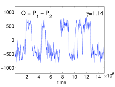
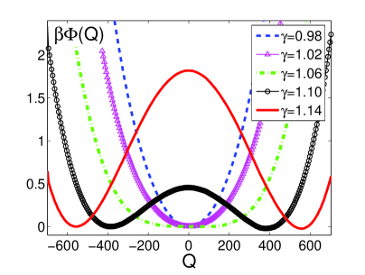
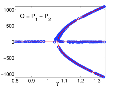
Figure 1: Summary of equation-free results from [13]. To compute the figures, we used model $(\ref{prodP1P2})$ – $(\ref{onoffO1O2})$ where equations $(\ref{prodP1P1P2P2})$ – $(\ref{onoffO1O2})$ were assumed to be at quasi-equilibrium, for parameter values see caption of Figure $5$ in [13].

stochastic model, while the upper right panel shows the effective free energy $\beta\Phi$ computed using (3.4) as the parameter $\gamma\equiv\gamma_{1}=\gamma_{2}$ is varied. The equation-free steady state distribution of $Q$ obtained from this effective free energy is in excellent agreement with histograms produced using long-time simulation (lower left panel). Equation-free computation has also been used [13] to compute “stochastic bifurcation diagrams” (an example is shown in the bottom right panel of Figure 1) using an extension of deterministic bifurcation computation [38]. We believe this array of equation-free numerical techniques holds promise for the acceleration of computer-assisted analysis of gene-regulatory networks. We now extend this analysis to systems where the “good” observables are unknown a priori by describing diffusion-map based variable-free methods.

4 Variable-free methods

4.1 Theoretical framework

To find a good, low ($n$-)dimensional representation of the full $N$-dimensional stochastic simulation data, we start by exploring the phase-space of most likely configurations of the system through extensive stochastic simulations; these configurations $\bf X$ (or a representative sampling of them) at, say $M$ different times are stored for processing. From $M$ such recordings we obtain a set of $M$ vectors $\bf{X}^{(1)},\ldots,\bf{X}^{(M)}$ in $\mathbb{R}^{N}$ which constitute the input to the diffusion map dimensionality reduction approach we will now describe. A crucial step for dimensionality reduction is the definition of a meaningful local distance measure between configurations. For continuous systems with equal noise strengths in all variables, one may use the following pairwise similarity matrix

$$\widetilde{W}_{ij}=\exp\left[-\left(\frac{\parallel\!\!{\bf X}^{(i)}-{\bf X}^{(j)}\!\!\parallel}{\sigma}\right)^{2}\right]$$ (4.1)

where $\parallel\!\!\cdot\!\!\parallel$ is the standard Euclidean norm in $\mathbb{R}^{N}$ and $\sigma$ is a characteristic scale for the exponential kernel which quantifies the “locality” of the neighborhood in which the Euclidean distance is considered (dynamically) meaningful [9].

For discrete chemical and biological reactions, as well as in other systems where the components of the data vectors may be disparate quantities varying over different orders of magnitude (possibly including even Boolean variables), the simple Euclidean norm in equation (4.1) with a single scaling factor $\sigma$ equal for all components may, of course, not be appropriate. In this case, it is reasonable to consider different scalings for the $N$ different components, using an $N$-dimensional weight vector

$${\mathbf{a}}=\left[a_{1},a_{2},\ldots,a_{N}\right]$$ (4.2)

where $a_{i}>0$, for $i=1,\dots,N$, and define a weighted Euclidean norm

$$\parallel\!\!{\bf X}\!\!\parallel_{\mathbf{a}}^{2}=\sum_{j=1}^{N}(a_{j}X_{j})^{2}.$$ (4.3)

This norm replaces the standard Euclidean norm in equation (4.1), where we may now choose $\sigma=1$, since this scaling can be absorbed into the vector ${\bf a}$; thus we replace (4.1) by

$$\widetilde{W}_{ij}=\exp\left[-\parallel\!\!{\bf X}^{(i)}-{\bf X}^{(j)}\!\!\parallel_{\mathbf{a}}^{2}\right].$$ (4.4)

The elements of the matrix $\widetilde{\mathbf{W}}$ are all less than or equal to one. Nearby points have $\widetilde{W}_{ij}$ close to one, whereas distant points have $\widetilde{W}_{ij}$ close to zero. In the diffusion map approach, given $\alpha\in[0,1]$ (the choice of this parameter value is discussed later), we define the matrix ${\bf W}$ by

$$W_{ij}=\left(\sum_{k=1}^{M}\widetilde{W}_{ik}\right)^{-\alpha}\left(\sum_{k=1}^{M}\widetilde{W}_{jk}\right)^{-\alpha}\widetilde{W}_{ij}$$ (4.5)

Next, we define a diagonal $M\times M$ normalization matrix $\bf D$ whose values are given by

$$D_{ii}=\sum_{k=1}^{M}W_{ik}$$ (4.6)

Finally we compute the eigenvalues and right eigenvectors of the matrix

$${\bf K}={\bf D}^{-1}{\bf W}.$$ (4.7)

In this paper we will mainly work with the parameter $\alpha=0$. However, in other applications different values of $\alpha$ may be more suitable (see Appendix A). As discussed in [30, 3, 29], if there exists a spectral gap among the eigenvalues of this matrix, then the leading eigenvectors may be used as a basis for a low dimensional representation of the data (see Appendix A). To compute these eigenvectors, we can make use of the fact that

$${\bf K}={\bf D}^{-1/2}{\bf S}{\bf D}^{1/2}\quad\mbox{ where }{\bf S}={\bf D}^{-1/2}{\bf W}{\bf D}^{-1/2}$$ (4.8)

is a symmetric matrix. Hence, $\bf K$ and $\bf S$ are adjoint and they have the same eigenvalues. Since $\bf S$ is symmetric, it is diagonalizable with a set of $M$ eigenvalues

$$\lambda_{0}\geq\lambda_{1}\geq\ldots\geq\lambda_{M-1}$$ (4.9)

whose eigenvectors ${\bf U}_{j}$, $j=1,\ldots,M$ form an orthonormal basis of $\mathbb{R}^{M}$. The right eigenvectors of $\bf K$ are given by

$${\bf V}_{j}={\bf D}^{-1/2}{\bf U}_{j}.$$ (4.10)

Since $\bf K$ is a Markov matrix, all its eigenvalues are smaller than or equal to one in absolute value. Moreover, if the parameter $\sigma$ in (4.1) is large enough (and, thus, the norm vector in (4.4) is “small enough”), all points are (numerically) connected and the largest eigenvalue $\lambda_{0}=1$ has multiplicity one with corresponding eigenvector

$${\bf V}_{0}=\left[1,1,\ldots,1\right].$$ (4.11)

We define the $n$-dimensional representation of $N$-dimensional state vectors by the following diffusion map

$$\Psi_{n}:{\bf X^{(i)}}\to\left[V^{(i)}_{1},V^{(i)}_{2},\ldots,V^{(i)}_{n}\right];$$ (4.12)

that is, the point ${\bf X}^{(i)}$ is mapped to a vector containing the $i$-th coordinate of each of the first $n$ leading eigenvectors of the matrix ${\bf K}$. This mapping $\Psi_{n}:\mathbb{R}^{N}\to\mathbb{R}^{n}$ is defined only at the $M$ recorded state vectors. We will show later that it can be extended to nearby points in the $N$-dimensional phase space, without full re-computation of a new matrix and its eigenvectors. In Appendix A we provide a theoretical justification for this method as a dynamically useful dimensionality reduction step.

4.2 Computation of data-based observables

We replaced (4.1) by (4.4) where the weight vector (4.2) needs to be further specified. Two natural choices for the values of components of the weight vector $\mathbf{a}=[a_{1},a_{2},\dots,a_{N}]$ immediately arise. One option is to regard the absolute values of the components of the state vector $\mathbf{X}$ as of “equal importance”, i.e.

$$a_{k}=\omega,\qquad\mbox{for}\quad k=1,2,\dots,N,$$ (4.13)

where $\omega$ is a single method parameter; this is identical to the use of a single $\sigma$ in equation 4.1, namely $\sigma=\omega^{-1}.$

The above approach uses the Euclidean distance between data vectors as the basis for graph Laplacian construction and eigenanalysis. In our case, the components of these vectors are concentrations of different species (e.g. integer numbers of protein molecules, each with its own range over the data set). Moreover, the data vectors contain integers (0 and 1) representing states of Boolean operators. This motivates a second natural choice of the weight vector $\mathbf{a}=[a_{1},a_{2},\dots,a_{N}]$. We rescale the state vector $X$ to span the symmetrical domain (cube) in $N$-dimensional space, i.e.

$$a_{k}=\frac{\widetilde{\omega}}{\displaystyle\max_{i}X_{k}^{(i)}-\displaystyle\min_{i}X_{k}^{(i)}},\qquad\mbox{for}\quad k=1,2,\dots,N,$$ (4.14)

where the maximum and minimum values are computed over all $i=1,\dots,M.$ Formula (4.14) implies that components of the vector $\mathbf{X}^{(i)}-\mathbf{X}^{(j)}$, $i,j=1,\dots,M,$ satisfy

$$X_{k}^{(i)}-X_{k}^{(j)}\in\left[-\widetilde{\omega},\widetilde{\omega}\right]\qquad\mbox{for}\;k=1,\dots,N,\;i,j=1,\dots,M.$$

The difference between (4.13) and (4.14) is that the first formula implicitly assumes that the fluctuations in different components of the state vector $\mathbf{X}$ are equally important, i.e. the absolute values of fluctuations are important. Formula (4.14) on the other hand implies that relative changes (compared to the maximal observed change) in each component are more representative than the absolute values of the changes. We will see below that (4.13) appears more suitable for our variable-free analysis.

4.2.1 Comparison of (4.13) and (4.14)

Using our illustrative gene regulatory network example (2.1) – (2.3) we now study the dependence of the eigenvectors of the matrix $\mathbf{K}$ on the weighting vector $[a_{1},a_{2},\dots,a_{N}]$. We run the long-time Gillespie based stochastic simulation of (2.1) – (2.3) to obtain a representative set of $M$ state vectors using the following dimensionless stochastic rate constants $\gamma_{1}=\gamma_{2}=1.14,$ $\varepsilon_{1}=\varepsilon_{2}=0,$ $\delta_{1}=\delta_{2}=7.5\times 10^{-4},k_{1}=k_{2}=10^{-3},$ $k_{-1}=k_{-2}=10,$ $k_{o1}=k_{o2}=0.4,$ $k_{-o1}=k_{-o2}=10.$ After removing initial transients, we started recording the values of the state vector (2.4) every $2\times 10^{8}$ SSA time steps. We made $2000$ recordings to obtain a data file with $M=2000$ state vectors. Next, we use these state vectors $\mathbf{X}^{(i)}$ to compute the $M\times M$ matrix $\mathbf{K}$ and its eigenvectors. We use formula (4.13) to compute $\mathbf{W}$ and $\mathbf{D}$ by (4.4), (4.5) and (4.6). Then we use implicitly restarted Arnoldi methods (ARPACK package [28]) to find the eigenvectors corresponding to the highest eigenvalues of the symmetric matrix $\mathbf{S}$ given by (4.8). Finally, we compute the eigenvectors of $\mathbf{K}=\mathbf{D}^{-1}\mathbf{W}$ by (4.10).

The formula (4.13) has a single parameter $\omega$ which is free for us to specify. It is easy to check numerically that the larger the “local neighborhood” size selected (that is, the smaller the $\omega$ value) the denser the connections between datapoints in the graph. Table 1 shows the highest eigenvalues for different values of $\omega$.

$\omega$ $\lambda_{0}$ $\lambda_{1}$ $\lambda_{2}$ $\lambda_{3}$ 0.02 1.00000 0.99986 0.94506 0.91360 0.01 1.00000 0.99920 0.77757 0.71122 0.005 1.00000 0.99279 0.44352 0.35515 0.002 1.00000 0.76262 0.10715 3.3 $\times 10^{-2}$ 0.001 1.00000 0.28346 1.2 $\times 10^{-2}$ 1.1 $\times 10^{-3}$ 0.0005 1.00000 7.5 $\times 10^{-2}$ 1.0 $\times 10^{-3}$ 1.5 $\times 10^{-4}$

Table 1: Top eigenvalues of matrix $\mathbf{K}$ computed using $(\ref{veca1})$ for $\alpha=0$ in $(\ref{weightmatrix})$.

We already know from [13] that the system is effectively one-dimensional. A good observable for the system is known to be $Q=P_{1}-P_{2}$, i.e. the difference between the first two coordinates of the state vector. However, the protein concentrations $P_{1}$ or $P_{2}$ were also found to give good equation-free results.

We plot the “empirical” good observable of each data point $i$ (its $P_{1}$ component, i.e. $X_{1}^{(i)}$, or the difference of its $P_{1}$ and $P_{2}$ components, i.e. $Q=X_{2}^{(i)}-X_{1}^{(i)})$ versus the one-dimensional representation $\Psi_{1}(\mathbf{X}^{(i)})$ (see (4.12)) of the point. The results are given in Figure 2 for two different values of $\omega$. The fact that the empirical coordinate $Q$ appears to effectively be one-to-one with the “automated” coordinate $\Psi_{1}(\mathbf{X}^{(i)})$ for all points in the data set confirms that $Q$ is indeed a good coordinate for data representation (the figure clearly shows $Q$ as the graph of a function above $\Psi_{1}(\mathbf{X}^{(i)})$, i.e. that the relation between $Q$ and $\Psi_{1}(\mathbf{X}^{(i)})$ is one-to-one). The $P_{1}$ vs. $\Psi_{1}(\mathbf{X}^{(i)})$ graph confirms that $P_{1}$ is also a good observable; it also is approximately one-to-one with $\Psi_{1}(\mathbf{X}^{(i)})$, yet the slightly “fat curve” suggests that $Q$ is a “better” observable.

$\omega=0.002$             $\omega=0.0005$

 

 

 

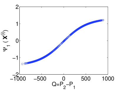
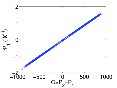
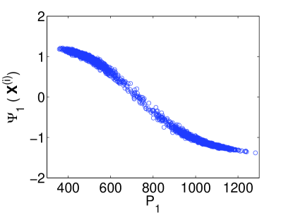
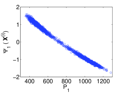
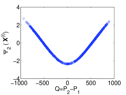
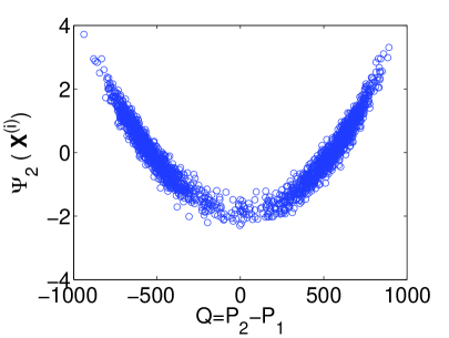
Figure 2: Variable-free results using formula $(\ref{veca1})$ and $\omega=0.002$ (left panels) or $\omega=0.0005$ (right panels). We plot $\Psi_{1}(\mathbf{X}^{(i)})$ which corresponds to eigenvalue $\lambda_{1}$ as function of $Q=P_{2}-P_{1}$ (top panels) and as function of $P_{1}$ (center panels). We also plot $\Psi_{2}(\mathbf{X}^{(i)})$ which corresponds to eigenvalue $\lambda_{2}$ as function of $Q=P_{2}-P_{1}$ (bottom panels).

The dependence of the variable-free results on the value chosen for $\omega$ may be rationalized through equation (4.1). As discussed in Section 4.2, our parameter $\omega$ is analogous to an inverse “cutoff length” in the computation of the diffusion map kernel; if it is too large, then the graph becomes disconnected. Clearly, it is a model parameter that has to be optimized depending on the problem; our results for $\omega=0.0005$ show a pure linear relation between the “empirical” $Q$ and the “automated” $\Psi_{1}(\mathbf{X}^{(i)})$ observables. Increasing $\omega$ by a factor of 2 corresponds to raising the elements of the matrix $\widetilde{\mathbf{W}}$ to the fourth power. This change in weight factor (followed by the normalization of (4.6)) leads to a different clustering of the data points. Large $\omega$ implies that Euclidean distances are meaningful when small; this results in a “more clustered” data set, where nearby data points (e.g. points within one potential well) appear (in diffusion map coordinates) relatively closer, while points far away (e.g. points in different potential wells) appear (in diffusion map coordinates) relatively more distant. Indeed, in the case of continuous variables, in the limit of large $\omega$ the eigenvectors of the diffusion map converge to the eigenfunctions of a corresponding Fokker-Planck diffusion operator. In the case of two deep potential wells, this eigenfunction is approximately constant in the two wells with a sharp transition between them. This might explain the slightly flat regions at the two edges of the apparent curve in the middle panel of Figure 2 for $\omega=0.002$; points within the same potential well may differ in $Q$, yet appear more nearby in the “automated” observable. We also include a plot of the relation between $Q$ and the component of the data in the second eigenvector $\Psi_{2}(\mathbf{X}^{(i)})$ for comparison.

Next we show that the weight vector computed using the formula (4.14) (based on the magnitude of relative state variable changes) is unsuitable for our variable-free analysis. We use the same set of $M=2000$ state vectors $\mathbf{X}^{(i)}$ to compute the $M\times M$ matrix $\mathbf{K}$ and its eigenvectors, using formula (4.14) to compute $\mathbf{W}$ and $\mathbf{D}$ by (4.4), (4.5) and (4.6). A single parameter $\widetilde{\omega}$ still remains to be specified in formula (4.14). We now again compare the “empirical” and “automated” observables of all data points ($Q=P_{1}-P_{2}$ as a function of $\Psi_{1}(\mathbf{X}^{(i)})$, the one-dimensional representation based on the first nontrivial eigenvector of the matrix $\mathbf{K}$). The results are given in Figure 3 for two different values of $\widetilde{\omega}$.

$\widetilde{\omega}=2$               $\widetilde{\omega}=0.1$

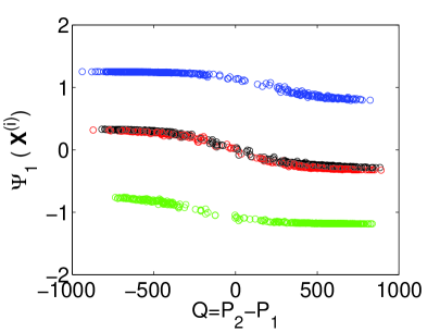
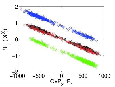
Figure 3: Variable-free results using formula $(\ref{veca2})$ and $\widetilde{\omega}=2$ (left panel) or $\widetilde{\omega}=0.1$ (right panel); datapoints colored according to gene states: black=$[0,0]$, green=$[0,1]$, blue=$[1,0]$, and red=$[1,1]$. We plot $\Psi_{1}(\mathbf{X}^{(i)})$ which corresponds to eigenvalue $\lambda_{1}$ as function of $Q=P_{2}-P_{1}$.

We see that the data split into four curves. Each curve corresponds to a distinct combination of gene operator states (actually, two of the curves effectively coincide). There are exactly four possibilities of gene states taken from the set

$$[O_{1},O_{2}]\in\Big{\{}[0,0],\;[0,1],\;[1,0]\;[1,1]\Big{\}}.$$

If we use formula (4.13), then the contribution of the distance between gene operator states to the data Euclidean distance is negligible compared to the fluctuations of the protein numbers. Local distances computed using the scaling in formula (4.14) are clearly not representative of the similarity of nearby (in this metric) points for the system dynamics: there is no one-to-one correspondence between the empirically known “good observable” $Q$ and the “automated” $\Psi_{1}(\mathbf{X}^{(i)})$ . Indeed, for the parameter values of our simulation, transitions between the 0 and 1 states of the operators are very fast (“easy”); on the other hand the Euclidean distance of two data points that differ only in these states is large when computed through the formula (4.14).

An alternative approach to computing the effective rate in (2.1) can be obtained assuming that the reaction (2.2) is fast and that we have a lot of protein molecules in the system. Then the quasi-steady state assumption gives the formula $\overline{P_{1}P_{1}}=2k_{1}/k_{-1}P_{1}^{2}$. Hence, we can write the number of dimers as a simple function of the number of monomer proteins. On the other hand, using the same approximation in equation (2.3), we obtain

$$O_{1}=\frac{k_{-o1}}{k_{o1}\overline{P_{2}P_{2}}+k_{-o1}}.$$ (4.15)

Equation (4.15) gives $O_{1}$ as a real number in the interval $[0,1]$. This number is a good approximation for computing the effective rate in (2.1). However, it is not a value of the Boolean variable $O_{1}$ – it is only a probability that the gene “is on” at the given time.

If, on the other hand, the “on-off” operator transitions were slow, then Figure 3 would be quite informative: it would suggest that we should augment our observables with the Boolean variables $O_{1}$, $O_{2}$, since these are “slow”. Because of the Boolean nature of the gene operator variables, it is not possible to know a priori how often these transitions occur, and, consequently, how to scale the quantized Boolean state distance so that it “meaningfully” participates in the Euclidean distance used for diffusion map analysis. As our diffusion map computations stand, we do not take into account the temporal proximity of points – when they have been obtained from the same transient. If such information is taken into account, it is conceivable that temporal proximity would provide guidance in choosing the components of weight vectors (especially for Boolean variables which change in a quantized manner) so that “local” Euclidean distances are indeed representative of the dynamical proximity between data points.

5 Variable-free computations

We now couple the above automated detection of observables with the equation-free computations in [13] in what we will refer to as “variable-free, equation-free” methods. The results in this section are for the model parameter values given in Section 4.2.1 using the weight vector defined by (4.13) with $\omega=0.0005$ and kernel parameter $\alpha=0$ (the standard, normalized graph Laplacian) in (4.5).

The data plot in terms of the observable $Q$ and the component in the eigenvector $\Psi_{1}(\mathbf{X}^{(i)})$ in Figure 2 suggested that a single diffusion map coordinate, denoted $Q_{dmap}\equiv\Psi_{1}(\mathbf{X}^{(i)})$, is sufficient to characterize the system dynamics. The diffusion map coordinate is found by performing the eigencomputations described in Section 4.1 using the full state vector ($N$=6) at each of the $M=2000$ recorded SSA datapoints (every $2\times 10^{8}$ SSA time steps) as input to our numerical routines.

In our previous paper [13] we described an approach to compute an effective free energy potential in terms of the observable $Q=P_{2}-P_{1}$. Variable-free computation of the effective free energy is now feasible using a similar approach modified to analyze simulation data in terms of the coordinate $Q_{dmap}$. Figure 4 plots the effective potential $\beta\Phi$ in terms of the automated reduction coordinate $Q_{dmap}$. To evaluate the effective drift ($V$) and diffusion ($D$) coefficients required in the construction of the effective free energy (equation (3.4)) we choose a value of $Q_{dmap}$, locate instances when it appears in the simulation database, record its subsequent evolution within a fixed time interval, and then average over these instances to estimate the rate of change in the mean and the variance. This procedure is repeated for a grid of $Q_{dmap}$ values enabling numerical evaluation of the integral in equation (3.4). The result of this analysis is compared in Figure 4 with the potential obtained by directly constructing the probability distribution $f(Q_{dmap})$ from the time series and employing the relationship $\beta\Phi(Q_{dmap})\sim-\log\left[f(Q_{dmap})\right]$.

Section 5.2 describes a lifting procedure that allows short bursts of simulation, instead of long time simulation, to be used in variable-free estimation of effective drift and diffusion coefficients.

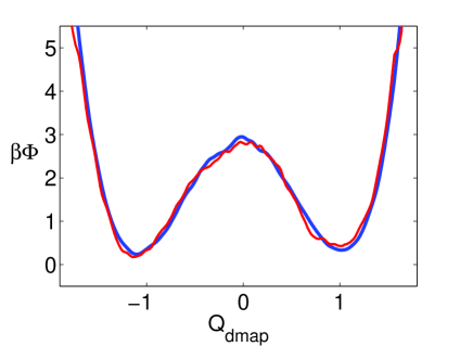
Figure 4: Effective free energy $\beta\Phi$ as a function of $Q_{dmap}$ from binning of all datapoints using an SSA database of $2^{37}$ time steps (blue lines) and computed from numerical integration of equation $(\ref{potentialPhi})$ using a $2^{34}$ point subsampling (keeping $1$ out of every $8$ points) of this database (red lines). Numerical integration performed using a more severe subsampling of the database with $2^{31}$ points produces an effective free energy profile with an unacceptable level of noise.

The central idea of “variable-free equation-free” methods is to perform equation-free analysis in terms of diffusion map variables, based on short bursts of SSA simulation in the original variables. This strategy requires an efficient means of converting between the physical variables of the system and those of its diffusion map (a restriction step) and vice versa: lifting from the diffusion map back to physical variables. For small sample sizes, eigendecomposition of the symmetric kernel $\mathbf{S}$ (defined in (4.8)) yields the diffusion map variables for each data point; yet, as the number of sample datapoints increases, the associated computational costs become prohibitive. The Nyström formula [2, 4] for eigenspace interpolation is a viable alternative to repeated matrix eigendecompositions for computing diffusion map coordinates of new datapoints generated during the course of a simulation. Eigenvectors and eigenvalues of the kernel $\mathbf{S}$ are related by $\mathbf{S}\mathbf{U}_{j}=\lambda_{j}\mathbf{U}_{j}$, or equivalently

$$U_{j}(\mathbf{X}^{(i)})=\frac{1}{\lambda_{j}}\sum_{k=1}^{M}S_{ik}U_{j}(\mathbf{X}^{(k)})$$ (5.1)

where $U_{j}(\mathbf{X}^{(i)})$ denotes the component of the $j^{th}$ eigenvector associated with state vector $\mathbf{X}^{(i)}$. Eigenvector components associated with a new state vector $\mathbf{X}^{new}$ cannot be computed directly from (5.1) because entries of the matrix $\mathbf{S}$ are defined only between pairs of datapoints in the original dataset. Defining the $M\times 1$ vector $\widehat{\mathbf{W}}^{new}$ of exponentials of the negative squares of the distances between the new point and database points by

$$\widehat{W}_{i}^{new}=\exp\big{[}-\parallel\!\!\mathbf{X}^{new}-\mathbf{X}^{(i)}\!\!\parallel_{\bf a}^{2}\big{]},$$ (5.2)

and the $M\times 1$ vector ${\mathbf{W}}^{new}$ by

$$W_{i}^{new}=\left(\sum_{k=1}^{M}\widetilde{W}_{ik}\right)^{-\alpha}\left(\sum_{k=1}^{M}\widehat{W}_{k}^{new}\right)^{-\alpha}\widehat{W}_{i}^{new},$$ (5.3)

allows the generalized kernel vector $\mathbf{S}^{new}$ to be defined as follows:

$$S_{i}^{new}=\left(\sum_{k=1}^{M}W_{ik}\right)^{-1/2}\left(\sum_{k=1}^{M}{W}_{k}^{new}\right)^{-1/2}{W}_{i}^{new}.$$ (5.4)

The entries in $\mathbf{S}^{new}$ quantify the pairwise similarities between the new point $\mathbf{X}^{new}$ and database points consistent with the definition of $\mathbf{S}$ in (4.8) [4].

5.1 Restriction from physical to diffusion map variables

The Nyström formula [2] is used to find the eigenvector component $U_{j}(\mathbf{X}^{new})$ associated with a new state vector $\mathbf{X}^{new}$

$$U_{j}(\mathbf{X}^{new})=\frac{1}{\lambda_{j}}\sum_{i=1}^{M}\widehat{S}_{i}^{new}U_{j}(\mathbf{X}^{(i)})$$ (5.5)

allowing the eigenvectors of the matrix $\mathbf{K}$ (and thereby the diffusion map coordinates) associated with $\mathbf{X}^{new}$ to be computed using (4.10). A full eigendecomposition is typically performed first for a representative subset of the (large) number of SSA datapoints and the Nyström formula is then used to perform the restriction operation in (5.5) which amounts to interpolation in the diffusion map space.

5.2 Lifting from diffusion map to physical variables

The process of lifting (shown schematically in Figure 5) consists of preparing a detailed state vector with prescribed diffusion map coordinates $Q_{dmap}^{targ}$. The main step in our lifting process is the minimization of a quadratic objective function defined as follows

$$Obj(Q_{dmap}(\mathbf{X}))=\lambda_{obj}(Q_{dmap}(\mathbf{X})-Q_{dmap}^{targ})^{2}$$ (5.6)

where $\lambda_{obj}$ is a weighting parameter that controls the shape of the objective away from its minimum at $Q_{dmap}(\mathbf{X}^{*})=Q_{dmap}^{targ}$. The implicit dependence of $Q_{dmap}$ on $\mathbf{X}$ makes this optimization problem nontrivial.

We use here, for simplicity, the method of Simulated Annealing (SA) [26, 31] to solve the optimization problem, and identify a value of the state vector $\mathbf{X}^{*}$ with the target diffusion map coordinates $Q_{dmap}^{targ}$. The SA routine [31] employs a “thermalized” downhill simplex method as the generator of changes in configuration. The simplex, consisting of $N+1$ vertices, each corresponding to a trial state vector, tumbles over the objective landscape defined by (5.6) sampling new state vectors as it does so. The control parameter of the method is the “annealing temperature” which controls the rate of simplex motion. At high temperatures the method behaves like a global optimizer, accepting many proposed configurations (even those that take the simplex uphill i.e. in the direction of increasing objective function value). At low temperatures a local search is executed and only downhill simplex moves are accepted.

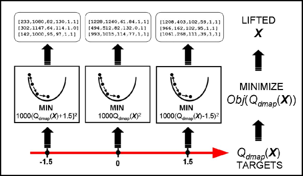
Figure 5: A schematic of the procedure for lifting from diffusion map coordinate $Q_{dmap}(\mathbf{X})$ to 6-dimensional state vector $\mathbf{X}$ via minimization of quadratic constraint potential $Obj(Q_{dmap}(\mathbf{X}))$. Target values of diffusion map coordinate are shown at the base of the figure, with the potential function to be minimized in each case indicated above these targets. For each diffusion map coordinate value shown, $3$ consistent state vectors (generated by lifting) are indicated at top of figure.

The starting simplex configuration for this $N$-parameter minimization may be selected at random or (more reasonably) by taking those state vectors in the existing database with diffusion map coordinates closest to the target $Q_{dmap}^{targ}$. It is important to note that the SA optimization scheme requires the Nyström formula at each iteration to compute $Q_{dmap}(\mathbf{X}^{trial})$ for trial state vectors, and thus evaluate the objective function value, which determines whether the configuration will be accepted or not. Once the objective has been evaluated at each of the starting vertices, the following steps are repeated until a minimum is located:

(a) Move the simplex to generate a new state vector $\mathbf{X}^{trial}$;

(b) Evaluate the objective function value at the new state vector $Obj(Q_{dmap}(\mathbf{X}^{trial}))$;

(c) Decrement the annealing temperature.

The downhill simplex method prescribes the motion in step (a) making a selection from a set of moves according to the local objective “terrain” (set of objective values at the vertices encountered). Step (b) requires an evaluation using the Nyström formula. We note here that this lifting strategy prepares state vectors with desired diffusion map coordinates using search algorithm “dynamics”. The suitability of this approach relative to alternatives that employ physical dynamics (e.g. using constrained evolution of the stochastic simulator in the spirit of the SHAKE algorithm in molecular dynamics [36]) is a relevant and interesting question that merits further investigation.

5.3 Illustrative Numerical Results

Equipped with restriction and lifting operators between physical and “automated” variables, we can now perform all the equation-free tasks of [13] in the diffusion map coordinate $Q_{dmap}$ i.e. in variable-free mode.

A procedure for variable-free computational estimation of $V(q)$ and $D(q)$ in (3.4) is as follows:

[A] At the value $Q_{dmap}=q_{dmap}$ lift to a consistent state vector using the approach described in Section 5.2.

[B] Use the state vector computed in step [A] as an initial condition for a short simulation burst and run multiple realizations for time $\Delta t$. Restrict the results of these simulations (Section 5.1) and use the definitions (3.2) and (3.3) (with $Q_{dmap}(t)$ instead of $Q(t)$) to estimate the effective drift $V(q_{dmap})$ and the effective diffusion coefficient $D(q_{dmap})$.

[C] Repeat steps [A] and [B] for sufficiently many values of $Q_{dmap}$ and then compute $\Phi(q)$ using formula (3.4) and numerical quadrature.

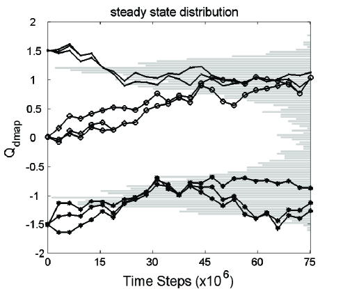
Figure 6: Drift in the diffusion map coordinates. The shaded horizontal boxes indicate the steady state probability distribution for $M=2000$. Points from SSA trajectories are shown at intervals of $3\times 10^{6}$. Initial configurations for these runs are those shown in Figure 5 prepared by lifting from $Q_{dmap}$ values of $(-1.5,0,1.5).$ Trajectories drift towards the most populated regions of the distribution.

We performed lifting for 3 values of the automated reduction coordinate ($Q_{dmap}=-1.5,0,1.5$), generating several replicas in each case. From Figure 6 it is apparent that the selected values of $Q_{dmap}$ are located near the “rims” of the wells of two local minima on the effective free energy landscape for this system. The state vectors generated by lifting are shown at the top of Figure 5. Figure 6 plots the SSA simulation evolution, initialized at these state vectors, in the observable $Q_{dmap}$. Also shown in Figure 6 is the steady state distribution in terms of $Q_{dmap}$ obtained from long SSA runs. Estimates for drift ($V$) and diffusion ($D$) coefficients at $Q_{dmap}$ values of -1.5 and 0 produced by sampling the simulation database and using the lifting procedure described in this paper are compared in Table 2. It should be possible to reach a better agreement between the coefficient estimates based on the long simulation database and those obtained by a lifting procedure if we evolve the actual model dynamics with a constraint on the prescribed $Q_{dmap}$ value - possibly through a parabolic constraint potential of the type used in umbrella sampling (see also the “run and reset” procedure described in [14, 13]). The effective free energy predicted by analyzing the full simulation database in terms of $Q_{dmap}$ can be found in Figure 4.

Database Lifting $(Q_{dmap})_{0}$ $V$ $D$ $V$ $D$ -1.5 3.3 $\times 10^{-5}$ 4.7 $\times 10^{-6}$ 2.1 $\times 10^{-5}$ 3.2 $\times 10^{-6}$ 0. 5.3 $\times 10^{-6}$ 4.0 $\times 10^{-6}$ 7.9 $\times 10^{-8}$ 4.1 $\times 10^{-6}$

Table 2: Estimates for drift ($V$) and diffusion ($D$) coefficients (in $s^{-1}$) at $Q_{dmap}$ values of $-1.5$ and $0$ using initial conditions drawn from the simulation database and prepared by lifting.

6 Summary and Conclusions

The knowledge of good observables is vital in our ability to create effective reduced models of complex systems, and thus to analyze and even design their behavior at a macroscopic/engineering level more efficiently. In this paper we illustrated a connection between computational data-mining (in particular, diffusion maps and the resulting low-dimensional description of high-dimensional data) with computational multiscale methods (in particular, certain equation-free algorithms). Our illustrative example consisted of a model gene regulatory network known to exhibit bistable (switching) behavior in some regime of its parameter space. We also presented examples of lifting and restriction protocols, that enable the passing of information between detailed state space and reduced “diffusion map coordinate” space. These protocols allow us to “intelligently” design short bursts of appropriately initialized stochastic simulations with the detailed model simulator. Processing the results of these simulations in diffusion coordinate space forms the basis for the design of subsequent numerical experiments aimed at elucidating long-term system dynamic features (such as equilibrium densities, effective free energy surfaces, escape times between different wells, and their parametric dependence). In particular, we confirmed that previously, empirically known, observables were indeed meaningful coarse-grained coordinates.

In traditional diffusion map computations, a single scalar (a scaled Euclidean norm) forms the basis for the identification of good reduced coordinates (when they exist). An important issue that arose in our example, due to the disparate nature, value ranges and dynamics of different data vector components, was the selection of appropriate relative scaling among data component values. The computational approach we used was based on the data ensemble, without any contribution from the dynamical proximity between data points collected along the same trajectory. We believe that incorporating such information will be very useful in determining relative scalings among disparate data components; finding ways to integrate such information among data ensembles collected in different experiments, and possibly with different sampling rates will greatly assist in this direction.

In this work, diffusion map computations were based on data collected from a single long transient, that was considered representative of the entire relevant portion of the (six-dimensional) phase space. In more realistic problems such long simulations will be no longer possible; yet local simulation bursts, observed on locally valid diffusion map coordinates can be used to guide the efficient exploration of phase space. Local smoothness in these coordinates allows us to use them in protocols such as umbrella sampling [41, 36] to “differentially locally extend” effective free energy surfaces. For example, “reverse coarse” integration described in [17, 15] provides computational protocols for microscopic/stochastic simulators to track backward in time behavior, accelerating escape from free energy minima and allowing identification of saddle-type coarse-grained “transition states”. Design of (computational) experiments for obtaining macroscopic information is thus complemented by the design of (computational) experiments to extend good low-dimensional data representations: both the coarse-grained coordinates and the operations we perform on them can be obtained through appropriately designed fine scale simulation bursts.

In this paper the connection between diffusion maps and coarse-grained computation operated only in one direction: diffusion map coordinates influenced the subsequent design of numerical experiments. An important current research goal is to establish the “reverse connection”: the on-line extension/modification of diffusion map coordinates towards sampling important, unexplored regions of phase space.

Appendix Appendix A Diffusion Maps

The following discussion is largely adapted from [3, 9]. We present a criterion for dimensionality reduction and show how it leads to the diffusion map method.

Suppose we have $M$ points ${\bf X}^{(i)}\in\mathbb{R}^{N}$, $i=1,\ldots,M$, and we define the matrix ${\bf W}$ by (4.5). Given a mapping ${\bf f}:[1,\ldots,M]\to\mathbb{R}^{n}$, we define the functional ${\cal L}$ by the formula

$${\cal L}({\bf f})=\sum_{i,j}\parallel\!\!{\bf f}(i)-{\bf f}(j)\!\!\parallel^{2}W_{ij}.$$ (A.1)

We see that ${\cal L}({\bf f})$ is always nonnegative. Moreover, $W_{ij}$ is close to (resp. far from) one for vectors ${\bf X}^{(i)}$ and ${\bf X}^{(j)}$ which are near (resp. far) from each other. For a dimensionality reduction function ${\bf f}$ to be useful, we must make sure that nearby points ${\bf X}^{(i)},{\bf X}^{(j)}$ in $\mathbb{R}^{N}$ are mapped to nearby points ${\bf f}({\bf X}^{(i)}),{\bf f}({\bf X}^{(j)})$ in $\mathbb{R}^{n}$. To find such a mapping, one can solve the following minimization problem

$$\arg\min_{{\bf f}\in\mathbb{F}}{\cal L}({\bf f})\quad\mbox{ where }\mathbb{F}=\{{\bf f}:{\bf F}^{T}{\bf D}{\bf F}={\bf I}_{n},{\bf F}^{T}{\bf D}{\bf 1}={\bf 0}\}$$ (A.2)

where ${\bf F}$ is the $M\times n$ matrix with row vectors ${\bf f}(i)$, ${\bf D}$ is the $M\times M$ diagonal matrix with entries $D_{ii}=\sum_{j}W_{ij}$ , $i=1,\ldots,M$, ${\bf I}_{n}$ is the $n\times n$ identity matrix, $\bf 1$ is a vector of $M$ ones, and ${\bf 0}$ a vector of $n$ zeros. The first constraint removes the arbitrary scaling factor, while the second constraint ensures that we do not map all $M$ points ${\bf X}^{(i)}$ to the same number. Since (A.1) can be rewritten as

$${\cal L}({\bf f})=\sum_{i,j=1}^{M}\parallel\!\!{\bf f}(i)-{\bf f}(j)\!\!\parallel^{2}W_{ij}=\mbox{tr}({\bf F}^{T}({\bf D}-{\bf W}){\bf F})$$ (A.3)

the solution ${\bf F}$ is given by the matrix of eigenvectors corresponding to the lowest eigenvalues of the matrix

$${\bf D}^{-1}[{\bf D}-{\bf W}]={\bf I}_{M}-{\bf K}$$ (A.4)

or equivalently by the largest eigenvalues of ${\bf K}$. By the non-negativity of the functional ${\cal L}({\bf f})$ it follows that the eigenvalues of ${\bf I}_{M}-{\bf K}$ are all non-negative, or that all eigenvalues of ${\bf K}$ are smaller than or equal to one. The eigenvector corresponding to the eigenvalue $\lambda_{0}=1$ is the vector ${\bf 1}$. Ordering the remaining eigenvectors in decreasing order we see that the $n$-dimensional representation of $N$-dimensional data points, via the minimization of (A.2) is the diffusion map (4.12).

We note that our $M$ points and the matrix $W_{ij}$ can be also viewed as the weighted full graph with $M$ vertices, where the weight associated with an edge between points $i$ and $j$ is equal to $W_{i,j}$. Then the previous analysis can be reformulated in terms of standard spectral graph theory [8, 3]. More precisely, it was shown in [29] that this construction leads to the classical normalized graph Laplacian for $\alpha=0$ in (4.5). If $\alpha=1$, then the construction gives the Laplace-Beltrami operator on the graph. Finally, if the data are produced by a stochastic (Langevin) equation, $\alpha=1/2$ provides a consistent method to approximate the eigenvalues and eigenvectors of the underlying stochastic problem.

Appendix Appendix B Simple Illustrative Examples

We include a brief illustration of the application of the diffusion map approach to the well known 3-dimensional “Swiss roll” data set [40, 35, 11] (shown in left panel of Figure 7) where datapoints lie along a 2-dimensional manifold. For this dataset $\mathbf{X}=\left[x,y,z\right]$; to compute the diffusion map we use $\alpha=1$, and $\sigma=2$ in equation (4.1). Figure 7 (right panel) plots these datapoints in terms of their components in the top two significant eigenvectors ($\Psi_{1}(\mathbf{X}^{(i)}),\Psi_{2}(\mathbf{X}^{(i)})$) of the matrix $\mathbf{K}$ for this dataset; it shows the “unrolled” 2-dimensional manifold detected by the diffusion map algorithm. The same result is obtained irrespective of the ordering (or orientation) of the dataset used to compute the pairwise similarity matrix.

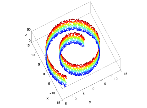
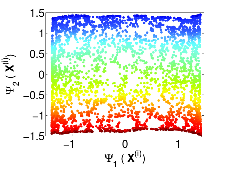
Figure 7: Left panel: Swiss roll dataset in $\mathbb{R}^{3}$. Datapoints lie along a $2$-dimensional manifold. Datapoints are colored by their $z$-coordinate value (ordering of datapoints passed to diffusion map routine is random). Right panel: plot of $\Psi_{1}(\mathbf{X}^{(i)})$ (corresponding to eigenvalue $\lambda_{1}$) against $\Psi_{2}(\mathbf{X}^{(i)})$ (corresponding to eigenvalue $\lambda_{1}$) for points in the dataset (same coloring scheme). The diffusion map “unrolls” the $2$-dimensional manifold.

As a second illustration, Figure 8 shows the potential

$$E(x,y)=\frac{x^{4}}{8}-x^{3}+2x^{2}+\frac{y^{4}}{5}+6\exp(-2(x-2)^{2}-10y^{2})$$ (B.1)

which has two minima connected by two paths. A subsampling of the dataset generated by Monte Carlo simulation using this potential is shown in Figure 9 (left panel) with the corresponding diffusion map shown in the right panel of the figure. For this dataset $\mathbf{X}=\left[x,y\right]$; to compute the diffusion map we use $\alpha=0$, and $\sigma=0.5$ in equation (4.1). Figure 9 (right panel) shows that points close to the bottom of the wells are mapped to tight clusters in the diffusion map, with a clear distinction between datapoints on each of the two transition pathways between the minima.

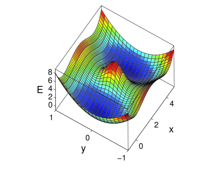
Figure 8: Two-well potential $(\ref{2wellPOT})$ with two connecting pathways between minima.

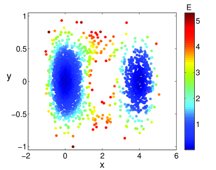
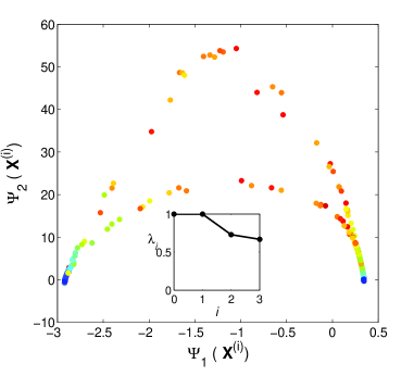
Figure 9: Left panel: Subsampled dataset generated by Monte Carlo simulation using potential defined in equation $(\ref{2wellPOT})$ (datapoints colored by energy according to colorbar). Right panel: dataset diffusion map (same coloring scheme) with top eigenvalues indicated in inset.

References

- [1] D. Adalsteinsson, D. McMillen, and T. Elston, Biochemical network stochastic simulator (BioNetS): software for stochastic modeling of biochemical networks, BMC Bioinformatics 5 (2004), no. 24, 1–21.
- [2] C. Baker, The numerical treatment of integral equations, Clarendon Press, Oxford, 1977.
- [3] M. Belkin and P. Niyogi, Laplacian eigenmaps for dimensionality reduction and data representation, Neural Computation 15 (2003), no. 6, 1373–1396.
- [4] Y. Bengio, O. Delalleau, N. Le Roux, J-F Paiement, P. Vincent, and M. Ouimet, Learning eigenfunctions links spectral embedding and kernel PCA, Neural Computation 16 (2004), no. 10, 2197–2219.
- [5] Y. Cao, D. Gillespie, and L. Petzold, The slow-scale stochastic simulation algorithm, Journal of Chemical Physics 122 (2005), 14116.
- [6] Y. Cao, D.T. Gillespie, and L. Petzold, Multiscale stochastic simulation algorithm with stochastic partial equilibrium assumption for chemically reacting systems, Journal of Computational Physics 206 (2005), 395–411.
- [7] S. Chatterjee, D. G. Vlachos, and M. A. Katsoulakis, Binomial distribution based -leap accelerated stochastic simulation, Journal of Chemical Physics 122 (2005), 024112.
- [8] F. Chung, A. Grigor’yan, and S. Yau, Higher eigenvalues and isoperimetric inequalities on riemannian manifolds and graphs, Communications on Analysis and Geometry 8 (2000), 969–1026.
- [9] R. Coifman, S. Lafon, A. Lee, M. Maggioni, B. Nadler, F. Warner, and S. Zucker, Geometric diffusions as a tool for harmonic analysis and structure definition of data: Diffusion maps, PNAS 102 (2005), 7426–7431.
- [10] , Geometric diffusions as a tool for harmonic analysis and structure definition of data: Multiscale methods, PNAS 102 (2005), 7432–7437.
- [11] D.L. Donoho and C. Grimes, Hessian eigenmaps: Locally linear embedding techniques for high-dimensional data, PNAS 100 (2003), 5591–5596.
- [12] W. E, D. Liu, and E. Vanden-Eijnden, Nested stochastic simulation algorithm for chemical kinetic systems with disparate rates, Journal of Chemical Physics 123 (2005), 194107.
- [13] R. Erban, I. Kevrekidis, D. Adalsteinsson, and T. Elston, Gene regulatory networks: A coarse-grained, equation-free approach to multiscale computation, Journal of Chemical Physics 124 (2006), 084106.
- [14] R. Erban, I. Kevrekidis, and H. Othmer, An equation-free computational approach for extracting population-level behavior from individual-based models of biological dispersal, Physica D 215 (2006), no. 1, 1–24.
- [15] T.A. Frewen, I. Kevrekidis, and G. Hummer, Equation–free exploration of coarse free energy surfaces, in preparation, 2006.
- [16] T. Gardner, C. Cantor, and J. Collins, Construction of a genetic toggle switch in e. coli, Nature 403 (2000), 339–342.
- [17] C. Gear and I. Kevrekidis, Computing in the past with forward integration, Physics Letters A 321 (2004), 335–343.
- [18] D. Gillespie, Exact stochastic simulation of coupled chemical reactions, Journal of Physical Chemistry 81 (1977), no. 25, 2340–2361.
- [19] , Approximate accelerated stochastic simulation of chemically reacting systems, Journal of Chemical Physics 115 (2001), no. 4, 1716–1733.
- [20] M. Haataja, D. Srolovitz, and I. Kevrekidis, Apparent hysteresis in a driven system with self-organized drag, Physical Review Letters 92 (2004), no. 16, 160603.
- [21] E. Haseltine and J. Rawlings, Approximate simulation of coupled fast and slow reactions for stochastic chemical kinetics, Journal of Chemical Physics 117 (2002), 6959–6969.
- [22] J. Hasty, D. McMillen, and J. Collins, Engineered gene circuits, Nature 420 (2002), 224–230.
- [23] G. Hummer and I. Kevrekidis, Coarse molecular dynamics of a peptide fragment: free energy, kinetics and long time dynamics computations, Journal of Chemical Physics 118 (2003), no. 23, 10762–10773.
- [24] T. Kepler and T. Elston, Stochasticity in transcriptional regulation: Origins, consequences and mathematical representations, Biophysical Journal 81 (2001), 3116–3136.
- [25] I. Kevrekidis, C. Gear, J. Hyman, P. Kevrekidis, O. Runborg, and K. Theodoropoulos, Equation-free, coarse-grained multiscale computation: enabling microscopic simulators to perform system-level analysis, Communications in Mathematical Sciences 1 (2003), no. 4, 715–762.
- [26] S. Kirkpatrick, C. Gelatt, and M. Vecchi, Optimization by simulated annealing, Science 34 (1983), no. 4598, 671–680.
- [27] D. Kopelevich, A. Panagiotopoulos, and I. Kevrekidis, Coarse-grained kinetic computations of rare events: application to micelle formation, Journal of Chemical Physics 122 (2005), 044908.
- [28] R. Lehoucq, D. Sorensen, and C. Yang, ARPACK users’ guide: solution of large-scale eigenvalue problems with implicitly restarted Arnoldi methods, SIAM, Philadelphia, USA, 1998.
- [29] B. Nadler, S. Lafon, R. Coifman, and I. Kevrekidis, Diffusion maps, spectral clustering and eigenfunctions of fokker-planck operators, Neural Information Processing systems 18 (2005), 819–851.
- [30] , Diffusion maps, spectral clustering and the reaction coordinates of dynamical systems, Applied and Computational Harmonic Analysis 21 (2006), 113–127.
- [31] W. Press, S. Teukolsky, W. Vetterling, and B. Flannery, Numerical Recipes, Cambridge University Press, 1992.
- [32] C. Rao and A. Arkin, Stochastic chemical kinetics and the quasi-steady-state assumption: application to the gillespie algorithm, Journal of Chemical Physics 118 (2003), 4999–5010.
- [33] M. Rathinam, L.R. Petzold, Y. Cao, and D.T. Gillespie, Stiffness in stochastic chemically reacting systems: The implicit tau-leaping method, Journal of Chemical Physics 119 (2003), 12784–12794.
- [34] H. Risken, The Fokker-Planck Equation, methods of solution and applications, Springer-Verlag, 1989.
- [35] S.T. Roweis and L.K. Saul, Nonlinear dimensionality reduction by locally linear embedding, Science 290 (2000), 2323–2326.
- [36] J. P Ryckaert, G. Ciccotti, and H.J.C. Berendsen, Numerical integration of the cartesian equations of motion of a system with constraints: molecular dynamics of n-alkanes, Journal of Computational Physics 23 (1977), 327–341.
- [37] H. Salis and Y. Kaznessis, Accurate hybrid stochastic simulation of a system of coupled chemical or biochemical reactions, Journal of Chemical Physics 122 (2005), 054103.
- [38] C. Siettos, M. Graham, and I. Kevrekidis, Coarse Brownian dynamics for nematic liquid crystals: Bifurcation, projective integration, and control via stochastic simulation, Journal of Chemical Physics 118 (2003), no. 22, 10149–10156.
- [39] S. Sriraman, I. Kevrekidis, and G. Hummer, Coarse nonlinear dynamics of filling-emptying transitions: water in carbon nanotubes, submitted to Physical Review Letters, 2005.
- [40] J.B. Tenenbaum, V. de Silva, and J.C. Langford, A global geometric framework for nonlinear dimensionality reduction, Science 290 (2000), 2319–2323.
- [41] G. M Torrie and J. P. Valleau, Monte Carlo free energy estimates using non-Boltzmann sampling: Application to the sub-critical Lennard-Jones fluid, Chemical Physics Letters 28 (1974), 578–581.