Exploring the assortativity-clustering space of a network’s degree sequence

Abstract

Nowadays there is a multitude of measures designed to capture different aspects of network structure. To be able to say if the structure of certain network is expected or not, one needs a reference model (null model). One frequently used null model is the ensemble of graphs with the same set of degrees as the original network. In this paper we argue that this ensemble can be more than just a null model—it also carries information about the original network and factors that affect its evolution. By mapping out this ensemble in the space of some low-level network structure—in our case those measured by the assortativity and clustering coefficients—one can for example study how close to the valid region of the parameter space the observed networks are. Such analysis suggests which quantities are actively optimized during the evolution of the network. We use four very different biological networks to exemplify our method. Among other things, we find that high clustering might be a force in the evolution of protein interaction networks. We also find that all four networks are conspicuously robust to both random errors and targeted attacks.

I Introduction

Network structure mejn:rev ; doromen:book ; ba:rev is usually defined as the way a network differs from what is expected. What “expected” means depends on the fundamental constraints on the network, and this can vary from system to system. For example, if the network is made of units that must be connected to two, and only two, others; then, it is not interesting whether or not a vertex lies on a cycle (we already know that it will). The ensemble of all networks fulfilling the fundamental constraints on the system is usually called null model (or reference model). When we have pinned down the null model we can measure the network structure by standard quantities. If the values of these quantities differs significantly from the null-model average, then we call the network structured. The baseline assumption of complex network theory is that network structure carries information about the forces that have formed the network. Ever since the studies of Barabási and coworkers ba:model ; ba:rev , the degree distribution (or, if referring to the set of degrees of one particular network, degree sequence) has been regarded as the most fundamental network structure. For many networks, the degrees are related to outer factors (not emerging from the network evolution). In such cases the ensemble of all graphs with the same degree sequence as the original network is a natural null model. Another interpretation is that the network structures measured relative to this null model are of higher order than the degree—i.e., what remain after the effects of the more fundamental structure (the degree sequence) is filtered away. The usual way to use a null model is to compare a network measure with the ensemble average value of the null model. In this paper we will argue that one can glean more information about the original network by studying the null model ensemble in greater detail than just measuring averages.

We consider networks that can be modeled as a graph $G=(V,E)$ where $V$ is the set of $N$ vertices and $E$ is the set of $M$ undirected edges. We denote the ensemble of graphs with the same degree sequence as $G$ as $\mathcal{G}(G)$. Our basic approach to study $\mathcal{G}(G)$ is to resolve its members in the space of higher order network structures. The two such higher order network structures we consider in this paper are: the correlation between the degrees at either side of an edge (measured by the assortative mixing coefficient, $r$ mejn:assmix , or simply assortativity); and, the fraction of triangles in the network (measured by the clustering coefficient, $C$ bw:sw ; mejn:rev ). By mapping out $\mathcal{G}(G)$ in the space defined by $r$ and $C$ one can pose questions such as: How large is the region in $r$-$C$ space where members of $\mathcal{G}(G)$ actually exist? (This helps us answer how constrained the network evolution is if the degrees are given.) Is the real network close to $\mathcal{G}(G)$’s boundaries in $r$-$C$ space? (Which would indicate whether or not $r$ or $C$ are actively optimized.)

The basis for our exploration of an ensemble $\mathcal{G}(G)$ is to map out its members in the space defined by some network-structural measures, in our case the assortativity and clustering. We explore the $r$-$C$ space by successively rewire pairs of edges, $(i,j)$ and $(i^{\prime},j^{\prime})$ to $(i,j^{\prime})$ and $(i^{\prime},j)$, that takes the system in a desired direction. Rewiring techniques for studying networks are half a century old gale:rew (randomization for obtaining null models was studied in Ref. katz:cug ). In the physics literature these techniques were first used in Refs. maslov:pro ; alon .

II Network structural measures

Before going into details of our algorithm, we will review the network structural quantities that we use to describe our networks: both the independent variables (the assortative and clustering coefficients) that form the basis for our space of interest; and the quantities we use for characterizing the regions of this space.

II.1 Assortative mixing coefficient

It is quite well accepted that the set of degrees, the degree sequence, is the network quantity that contains most information about both the evolution and function of the network. Degree can (in most contexts) be identified as how influential the vertex is wf (in some sense)—high degree vertices are assumed to be more influential both the formation of the network and the flow of dynamic systems on the network. In this paper we assume the degree sequence is inherent to the system and look at higher order structures arising from how the vertices are linked to one another. The simplest such higher-order structure is the correlations between the degrees of vertices at either side of an edge. Is it the case that high-degree vertices are primarily connected to other high degree vertices, or are they linked to low-degree vertices? A simple way of measuring this tendency is by the assortativity mejn:rev $r$. Basically speaking, $r$ is the linear correlation coefficient of the degrees at either side of an edge. One complication is that since the edges are undirected, $r$ has to be symmetric with respect to edge-reversal, but the correlation coefficient is not symmetric. The solution is to let one edge contribute twice to the covariance, i.e. represent an undirected edge by two directed edges pointing in opposite directions. If one use an edge list representation internally (i.e., let the edges be stored in an array of ordered pairs $(i_{1},j_{1}),\cdots,(i_{M},j_{M})$) then mejn:assmix

$$r=\frac{4\langle k_{1}\,k_{2}\rangle-\langle k_{1}+k_{2}\rangle^{2}}{2\langle k_{1}^{2}+k_{2}^{2}\rangle-\langle k_{1}+k_{2}\rangle^{2}}$$ (1)

where, for an edge $(i,j)$, $k_{1}$ is the degree of first argument (i.e., the degree of $i$) and $k_{2}$ is the degree of the second argument. The range of $r$ is $[-1,1]$ where negative values indicate a preference for high connected vertices to attach to low-degree vertices, and positive values means that vertices tend to be attached to others with degrees of similar magnitudes.

II.2 Clustering coefficient

Several simple random network models (such as the Edrős-Rényi er:on or the model for generating networks of a given $r$-value in Ref. mejn:assmix ) have rather few triangles (fully connected subgraphs of three vertices). For some classes of real-world networks (notably social networks holl:72 ) there is a strong tendency for triangles to form, which makes such models fail. The network measure of the density of triangles is called clustering coefficient. We use the definition of Ref. bw:sw :

$$C=3n_{\mathrm{triangle}}\>\big{/}\>n_{\mathrm{triple}},$$ (2)

where $n_{\mathrm{triangle}}$ is the number of triangles and $n_{\mathrm{triple}}$ is the number of connected triples (subgraphs consisting of three vertices and two or three edges). The factor three is included to normalize the quantity to the interval $[0,1]$.

II.3 Distance and component size

Two quantities that are, perhaps more than any other, related to the functionality of dynamic processes on the network are the relative size of the largest component (connected subgraph) $s$, and the average distance $\langle d\rangle$. $s$ is simply defined as the number of vertices in the largest component divided by $N$. The distance $d(i,j)$ between two vertices $i$ and $j$ is defined as the number of edges in the shortest path between these two vertices. $\langle d\rangle$ is $d(i,j)$ averaged over all vertex pairs ($i\neq j$) in the largest component. In a network with large $s$ and small $\langle d\rangle$, spreading processes will be fast and far-reaching. This is a good property of information networks, but bad in the context of, for example, disease spreading. Some authors have combined the distance and component size aspects by considering the average reciprocal distances our:attack ; latora:eff . For most purposes, we believe, valuable information gets lost in such a combination (a fragmented network $G$ with short average distances can be something very different from a connected graph of large distances and the same average reciprocal distances as $G$).

II.4 Robustness

One line of complex network research is the study of the response of the network to attacks, errors, failures and other events that effectively change the structure. The error response problem is usually formulated as: how does the functionality of the network change if a random fraction of the vertices, or edges, is removed mejn:rev ? The attack problem is the same, except that the vertices are not selected randomly but according to some strategy intended to decrease the networks’ functionality as rapidly as possible our:attack ; alb:attack . A frequently used metric for functionality is the ratio of $s$ before and after the event our:attack ; alb:attack ; motter:cascade . In the error and attack robustness problems, this quantity is typically plotted as a function of the number of removed vertices. The idea is that even if one network $G$ is more robust than another network $G^{\prime}$ to the removal of, say, $1\%$ of the vertices, $G^{\prime}$ can be less vulnerable than $G$ if $10\%$ of the vertices are deleted. Since we aim at mapping out the $r$-$C$ space of degree sequences, we would like to capture the robustness with just one number. We will use what we call the $f$-robustness $R_{f}$ of a network as the expected fraction of vertices that needs to be removed for the relative size of the largest component to decrease to a fraction $f\in(0,1)$ of its original value. The way of removal can either be random (the error problem) or selective (the attack problem). For the rest of the paper we will set $f=1/2$, and refer to the $1/2$-robustness just as “robustness” $R$. Other $f$-values give slightly different results, but our conclusions will hold for a range of intermediate $f$-values.

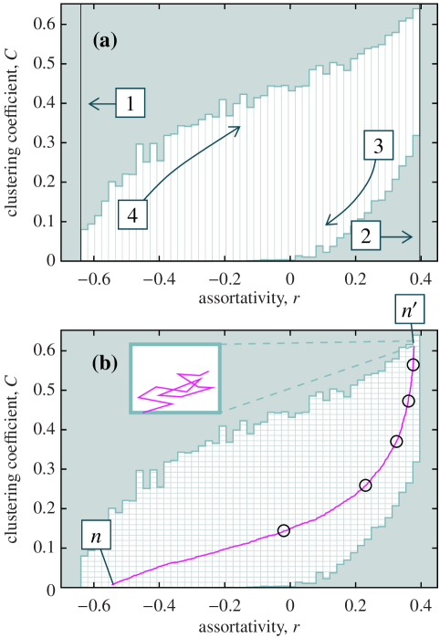
Figure 1: Illustration of the analysis scheme applied to the C. elegans neural network. (a) shows how the valid region is mapped out: 1. $r_{\mathrm{min}}$ is located. 2. $r_{\mathrm{max}}$ is found and the interval $[r_{\mathrm{min}},r_{\mathrm{max}}]$ is divided into $L$ segments. 3. $C_{\mathrm{min}}(n)$ is constructed. 4. $C_{\mathrm{max}}(n)$ is traced and the interval $[C_{\mathrm{min}},C_{\mathrm{max}}]$ is segmented into $L$ regions. (b) illustrates the sampling of the pixels. The next pixel to go to is chosen from a random permutation of the pixels. In this example $n$ and $n^{\prime}$ are chosen to be far apart. The line shows the path taken by the algorithm. The circles indicate every thousandth step on the way from $n$ to $n^{\prime}$. The blow-up illustrates the random walk within a pixel to sample the graphs of the pixel more randomly.

III The analysis scheme

The fundamental idea of our method is simple: we update the network by choosing pairs of edges randomly, say $(i,j)$ and $(i^{\prime},j^{\prime})$, and swap one end of them (forming $(i,j^{\prime})$ and $(i^{\prime},j)$). This guarantees that the degree sequence stays intact. We navigate in the $r$-$C$ space by only accepting changes that move us in the desired direction. If an edge-swap would introduce a self-edge (i.e. if $i=j^{\prime}$ or $i^{\prime}=j$) or a multiple edge (i.e. if $(i,j^{\prime})$ or $(i^{\prime},j)$ belongs to $E$ before the swapping, or move) it is not performed. There are many other technicalities concerning the convergence to extremes, uniformity of the sampling and more that we discuss in the Appendix.

The members of the ensemble $\mathcal{G}(G)$ do not, in general, cover the whole range of $(r,C)$-values. Indeed, for any finite $G$, $\mathcal{G}(G)$ defines a set of points, rather than a continuous region, in the $r$-$C$ space. We will perform a more coarse-grained analysis breaking down the $r$-$C$ space into pixels and average quantities over the graphs of $\mathcal{G}(G)$ with $(r,C)$-values within the pixel. (Thus, a pixel constitute a graph ensemble in itself, our aim is to sample its members with uniform randomness.) For a computationally tractable resolution, the pixels containing members of $\mathcal{G}(G)$ typically form contiguous regions. We will refer to the pixels that contain a member of $\mathcal{G}(G)$ as valid pixels, and all pixels that are valid or between valid pixels the valid region of $\mathcal{G}(G)$.

To trace the valid region of $\mathcal{G}(G)$ we start by finding the lowest and highest assortativity value, $r_{\mathrm{min}}$ and $r_{\mathrm{max}}$ respectively. Briefly speaking (more details follow below), to find $r_{\mathrm{min}}$ we rewire edge-pairs that lower $r$ (and vice versa for $r_{\mathrm{max}}$). After finding the extremal $r$-values, we splice the region between these into $L$ segments. Then we go through the region and for each region $n\in[1,L]$ we find the minimal and maximal $C$-values, $C_{\mathrm{min}}(n)$ and $C_{\mathrm{max}}(n)$. The region in $C$-space between the lowest $C_{\mathrm{min}}=\min_{1\leq n\leq L}C_{\mathrm{min}}(n)$ and highest $C_{\mathrm{max}}=\max_{1\leq n\leq L}C_{\mathrm{max}}(n)$ observed clustering coefficient is segmented into $L$ regions. (Note that $C_{\mathrm{min}}$, without argument, is the global clustering minimum, whereas $C_{\mathrm{min}}(n)$ is the minimum conditioned on $r$ being in the $n$’th segment.) Thus we (assuming our method works) obtain an $L\times L$ grid of the $r$-$C$ space that contains the valid region of $\mathcal{G}(G)$. The method is illustrated in Fig. 1.

To find the $\mathcal{G}(G)$ elements of minimal and maximal assortativity is a non-trivial optimization problem. There are deterministic methods that, if they terminate, are guaranteed to give the maximal (or minimal) assortativity doyle:big ; zj:spectrum . To avoid the such technicalities and to simplify the program, we will use the same kind of optimization algorithm to find $r_{\mathrm{max}}$ and $r_{\mathrm{min}}$ as to find $C_{\mathrm{min}}(n)$ and $C_{\mathrm{max}}(n)$. In the Appendix we will argue that this method allows us to come as close to the optimal $r$-values as we need. A method we find efficient is to repeat the simple edge-pair swapping procedure (where only changes in the desired direction are accepted) with different random seeds until no lower state is found during a number $\nu_{\mathrm{rep.}}$ of repetitions walker_walstedt . Each individual edge-pair is terminated when no lowest state is found for $\nu_{\mathrm{same}}$ swaps. In general, the larger the network is, the more densely distributed are the points close to the border of the valid region. If one is satisfied with finding a value a certain distance from the extrema, then $\nu_{\mathrm{rep.}}$ and $\nu_{\mathrm{same}}$ do not need to be increased for larger $N$. To find $C_{\mathrm{min}}(n)$ and $C_{\mathrm{max}}(n)$ almost the same procedure is employed. First, edge-pairs are swapped until the desired segment of $r$ is found. Second, unless $r$ is outside the segment $n$ and the move takes the system yet further from segment, edge-pairs are swapped provided the clustering would decrease (for $C_{\mathrm{min}}(n)$), or increase, (for $C_{\mathrm{max}}(n)$). When the valid region is traced out and we sample networks of different pixels, we select the pixels randomly. The idea is to sample the space of networks more randomly.

To summarize, the algorithm for finding the extremal assortativity values, $r_{\mathrm{min}}$ and $r_{\mathrm{max}}$, is:

1. Choose two undirected edges $(i,j)$ and $(i^{\prime},j^{\prime})$ at random. If the program makes a difference between the arguments of the edge, the direction of the reading of the edge also has to be randomized (so $(i,j)$ is read as $(j,i)$ with probability $1/2$).

2. Check if swapping these edges to $(i,j^{\prime})$ and $(i^{\prime},j)$ would introduce a self-edge or multiple edge in the network. If so, go to step 1.

3. Let $\Delta r$ be the change in $r$ if the move in step 1 is executed. If $r$ is to be minimized and $\Delta r<0$, then accept the change (vice versa for maximization of $r$).

4. If no move has been executed during the last $\nu_{\mathrm{same}}$ executions of step 3, then take the current $r$ as $\tilde{r}_{\mathrm{min}}$ (or $\tilde{r}_{\mathrm{max}}$).

5. Repeat from the beginning $\nu_{\mathrm{rep.}}$ times and return the lowest observed $\tilde{r}_{\mathrm{min}}$ during these iterations.

Given $r_{\mathrm{min}}$ and $r_{\mathrm{max}}$, and a division of the $r$ space into $L$ segments of width $(r_{\mathrm{max}}-r_{\mathrm{min}})/L$, we trace the boundaries of the valid region as follows:

1. Go through the regions sequentially. Say the $n$’th region is the interval $[r_{n},r_{n+1})$.

2. Perform step 1 and 2 of the assortativity optimization algorithm.

3. Let $\Delta C$ be the change in clustering coefficient during the previous step. If $r<r_{n}$ and $\Delta r>0$, $r\geq r_{n+1}$ and $\Delta r<0$ or $r_{n}\leq r<r_{n+1}$ and $\Delta C<0$ (for minimization) or $\Delta C>0$ (for maximization), then perform the change of step 6.

4. If, counting from the first time the system entered the desired $r$-segment, the minimal (maximal) $C$-value has been repeated $\nu_{\mathrm{same}}$ times, take this value as $\tilde{C}_{\mathrm{min}}(n)$ ($\tilde{C}_{\mathrm{max}}(n)$).

5. Repeat from step 6 $\nu_{\mathrm{rep.}}$ times. Let the lowest $\tilde{C}_{\mathrm{min}}(n)$-values and largest $\tilde{C}_{\mathrm{max}}(n)$ during these iterations be $C_{\mathrm{min}}(n)$ and $C_{\mathrm{max}}(n)$.

Then, when the valid region is mapped out, we split the $C$-range (between $C_{\mathrm{min}}$ and $C_{\mathrm{max}}$ in $L$ segments of equal width, thus forming an $L\times L$-grid enclosing the valid region. This grid is sampled as follows:

1. Construct a random permutation of the valid pixels.

2. Pick the next pixel $P_{n}=[r_{n},r_{n+1})\times[C_{m},C_{m+1})$ from the index-list of step 11. Denote the center $[(r_{n}+r_{n+1})/2,(C_{m}+C_{m+1})/2)]$ of the pixel $(r_{n,0},C_{m,0})$. Let

   $$\delta(r,C)=\sqrt{\left(\frac{r-r_{n,0}}{r_{\mathrm{max}}-r_{\mathrm{min}}}\right)^{2}+\left(\frac{C-C_{m,0}}{C_{\mathrm{max}}-C_{\mathrm{min}}}\right)^{2}}$$ (3)

   measure the distance in $r$-$C$ space from the current position $(r,C)$ to the center of the target pixel.

3. Pick edge-pair candidates according to steps 1 and 2 of the assortativity optimization algorithm.

4. Calculate $\Delta(r,C)=\delta(r^{\prime},C^{\prime})-\delta(r,C)$ where $r$ and $C$ are the current assortativity and clustering values, and $r^{\prime}$ and $C^{\prime}$ are the values after the pending move has been performed. If $\Delta(r,C)<0$ perform the move.

5. If the updated $(r,C)$ belongs to $P_{n}$, then: First, make $\nu_{\mathrm{rnd.}}$ random edge swappings such that $(r,C)$ does not leave $P_{n}$. (This is to sample the pixel more uniformly.) Then, measure network structural quantities of $P_{n}$, save these values for statistics, and go to step 12.

6. If not all pixels have been measured go to step 12.

7. Go to step 11 until each pixel have been sampled $\nu_{\mathrm{samp.}}$ times.

The parameter values we use in this study are (unless otherwise stated): $\nu_{\mathrm{same}}=10^{5}$, $\nu_{\mathrm{rep.}}=5$, $\nu_{\mathrm{samp.}}=100$, $\nu_{\mathrm{rnd.}}=1000$ and $L=50$. The choice of parameters and further considerations are discussed in the Appendix. Due to the uncertain stopping conditions of steps 4, 5, 9 and 10 it is hard to derive meaningful bounds on the computational complexity. We note, however, that the optimization is faster in $r$- than in $C$-direction, this probably relates to the observation in Fig. 1(b) that swapping procedure moves faster in the $r$- than in the $C$-direction. (The speed in the $C$-direction is roughly the same per 1000 steps, but the speed in the $r$-direction decrease.)

IV Networks

Our method can be applied to every kind of system that can be modeled as an undirected network. To limit ourselves, we use four networks from biology as examples in this paper. These networks are, nonetheless, representing fundamentally different systems.

Table 1: Basic statistical properties of the example networks we use. The number of vertices $N$, number of edges $M$, assortativity $r$, clustering coefficient $C$, relative size of the largest cluster $s$, average distance in the largest cluster $\langle d\rangle$, the error robustness $R_{\mathrm{error}}$ and the attack robustness $R_{\mathrm{attack}}$.

	gene fusion	protein interaction	metabolic	neural
$N$	$291$	$4168$	$1905$	$280$
$M$	$278$	$7434$	$3526$	$1973$
$r$	$-0.36$	$-0.13$	$-0.10$	$-0.069$
$C$	$0.0016$	$0.034$	$0.039$	$0.20$
$s$	$0.38$	$0.94$	$0.87$	$1$
$\langle d\rangle$	$4.2$	$4.8$	$4.5$	$2.6$
$R_{\mathrm{error}}$	$0.43$	$0.36$	$0.36$	$0.50$
$R_{\mathrm{attack}}$	$0.012$	$0.048$	$0.046$	$0.38$

IV.1 Gene fusion network

Cancer is a disease that occurs due to changes in the genome. One important process causing such changes is gene fusion—when two genes merge to form a hybrid gene mitelman . In Ref. hoglund the authors construct a network of human genes that have been observed to be fused in the development of tumors in humans. Some genes can fuse with many others but most of the genes have only been observed fusing with one, or a few others. The resulting network structure has a skewed, power-law like degree distribution and is rather fragmented—the largest component spanning only $38\%$ of the vertices. Statistics of this and the other networks are listed in Table LABEL:tab:stat.

IV.2 Metabolic network

A cell can be regarded as a machine driven by biochemical reactions. The possible reactions of the metabolism (the cellular biochemistry except signaling processes) and its environment determine the state of the cell. The metabolism of an organism is a very complex system—so complex that one has to choose between studying a part of it in detail, or the whole with a coarser method. One approach in the latter category is to construct a network, connecting the chemical substrates occurring in the same reactions to a network, and employ network analysis to characterize the large-scale structure of the metabolism. The way to construct a biochemical network is not entirely straightforward zhao:meta . Should the substances be linked to each other (in a substrate graph), or to the reactions they participate in? If one use a substrate graph, should the substrates be linked only to products, or to all reactants (i.e. in a reaction A + B $\leftrightarrow$ C + D, should A be linked to C and D, or to all three other vertices)? Furthermore, some chemical substances (like H₂O, ATP, NADH, and so on) are abundant throughout the cell and seldom pose any restriction on the reaction dynamics. For many purposes, one obtains a more meaningful network by deleting such currency metabolites. The biochemical network we use is the human metabolic network of Ref. our:curr . In this network, substrates are linked only to products (A to C and D in the above example). Currency metabolites are identified and deleted according to a self-consistent, graph-theoretic method our:curr .

IV.3 Protein interaction

In protein interaction networks the vertices are proteins and two proteins constitute an edge if they can interact physically. Examples of interaction are the ability to form complexes, carrying another protein across a membrane or modifying another protein. We use the (“physical interaction”) data set from Ref. hh:pfp of protein interaction in the budding yeast S. cerevisiae.

IV.4 Neural network

For the biochemistry of an organism, the network representation is a crude model of the system as a whole (as an alternative to a detailed model of a subsystem). Neural networks are yet more complex. For these the choices are either to make a coarse-grained network representation sporns:cortex or study the full network of a very simple organism. In this work, we take the latter approach and study the neural network of C. elegans white:420 . In this data set, the strength of the neuronal coupling has been measured, but we make the network undirected by letting an edge represent a non-zero coupling.

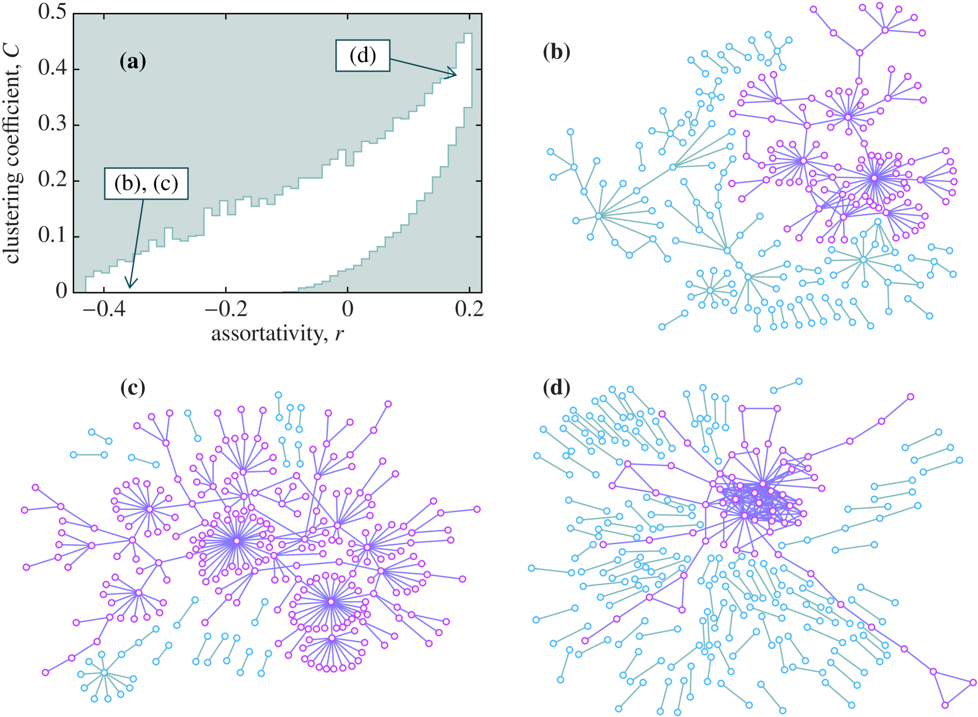
Figure 2: The valid region demarcated by the $C_{\mathrm{min}}(r)$- and $C_{\mathrm{max}}(r)$-curves (a), and three networks: (b) is the original gene fusion network, (c) shows a random sample with $r$-$C$ coordinates close to those of the real network. (d) shows a network with high clustering and high assortativity. The largest component of (b), (c) and (d) are indicated with a different color.

V Numerical results

In this section we present numerical results for our four network-structural measures over the $\mathcal{G}(G)$ ensembles of the four test graphs. To get a first view, we display the valid region of the gene fusion graph in Fig. 2(a). As seen, the valid region is not covering a large part of the theoretical limits of $r$ ($-1\leq r\leq 1$) and $C$ ($0\leq C<1$). (Note that only fully connected graphs have $C=1$, and for these $r$ is undefined.) The requirement that the graph should be simple (no multiple edges or self-edges) puts hard constraints on the actual $r$-values that can occur (cf. Ref. maslov:inet ). Fig. 2(a) shows that, considering the entire $r$-$C$ plane, such constraints are even harder. The general shape of the valid region is consistent with the observations that the simple-graph constraint induce a positive correlation between $r$ and $C$ maslov:inet ; mejn:why .

In Fig. 2(b), (c) and (d) we show three example networks of $\mathcal{G}(G)$ (where $G$ is the gene fusion network). Fig. 2(b) displays the relatively fragmented real network. Fig. 2(c) is a random network $G^{\prime}$ with the almost the same $r$-$C$ coordinates as the real network ($\delta(G,G^{\prime})\approx 0.0026$). Maybe the biggest visible difference between $G$ and $G^{\prime}$ is the larger size of the largest component of $G^{\prime}$. Is it true that the gene fusion network is unusually fragmented, given the degree sequence and $r$-$C$ coordinates? If so, there might be an evolutionary pressure for gene fusion networks to be fragmented. (This will be discussed further in Sect. V.1.) Fig. 2(d) shows, as a contrast, a network far away from $G$ and $G^{\prime}$. The network has a well-defined core where high-degree vertices connect to each other. There are also a number of peripheral triangles, which indicates that the network evolves toward a maximal $C$-value, given its assortativity.

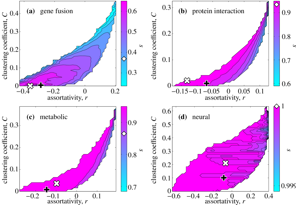
Figure 3: The relative size of the largest component $s$ as a function of $r$ and $C$. The networks are (a) the network of gene fusions in tumors in humans, (b) protein interaction network of S. cerevisiae, (c) human metabolic network and (d) the C. elegans neural network. The x-like symbols of the main figures and the diamond symbols of the color-bars indicate the values of the real networks. The plus-like symbol indicates the average $(r,C)$-value of the $\mathcal{G}(G)$ ensemble.

V.1 Location in $r$-$C$ space and size of largest component

In Fig. 3 we plot the relative size of the largest component of the four test networks. We also display the locations of the actual networks in the $r$-$C$ plane, and the $\mathcal{G}(G)$-averages. (The $\mathcal{G}(G)$ averages are obtained from a rewiring sampling of $\mathcal{G}(G)$, with step 2 of the algorithm as the only constraint.) We see that the $C$-value of the gene fusion graph lies close to the $C_{\mathrm{min}}(r)$-boundary of its valid region. $C$ averaged over the whole $\mathcal{G}(G)$ is about three times larger ($\langle C\rangle_{\mathcal{G}(G)}=0.0061\pm 0.0001$) than the observed value ($C=0.0017$). Furthermore, we see that the assortativity is lower than the $\mathcal{G}(G)$ average. This kind of analysis has been used by many authors (following Ref. maslov:pro ). The interpretation is usually that the network is, effectively, disassortative and clustered (i.e., $r<\langle r\rangle_{\mathcal{G}(G)}$ and $C>\langle C\rangle_{\mathcal{G}(G)}$). However, looking at the entire valid region, we can get another perspective: If high clustering really would have been an important goal for the network to obtain (given the degree sequence) there is large room for improvement. For the assortativity, on the other hand, the observed network is rather close to the minimum. This might be telling us that assortativity is a more important factor, than clustering, in the evolution of the gene fusion networks. The protein interaction network of Fig. 3(b) is located quite far from the ensemble average—the assortativity is much lower than the $\mathcal{G}(G)$-average, and given that assortativity, the clustering is maximal. Also the metabolic (Fig. 3(c)) and neural (Fig. 3(d)) networks are more clustered than the average, but here the assortativity is slightly larger than the $\mathcal{G}(G)$ average. From Fig. 3 we also note that the density of states is very inhomogeneous distributed—the average $(r,C)$ is close to $C=0$ and (except for the neural network) left of the middle of the assortativity spectrum. The shapes of the valid regions are rather similar, with an exception for the broader region of the neural network. This can be related to the more narrow degree sequence of the neural network amaral:classes . We have established a correlation between $r$ and $C$. Ref. mejn:why argues that such correlation occurs in social networks because of their modularity (or “community structure” as the authors call it). However, our large-$r$ networks have no explicit bias towards high modularity, which leads us to conjecture that the correlation between $r$ and $C$, or more fundamentally the sum $\sum_{(i,j)\in E}k_{i}k_{j}$ (which, given a degree sequence, is the only factor of Eq. 1 that can vary) is a more general phenomenon. Since $r$ is normalized by, essentially, the variance of the degree, it follows that the valid region for $\mathcal{G}(G)$ with more narrow degree sequence will appear stretched (larger).

Turning to the average size of the largest component, we observe that the gene fusion network is indeed more fragmented than the average network of the same $(r,C)$-coordinates (as anticipated from comparing Figs. 2(b) and (c)). The protein interaction and neural networks have no particular bias in this respect, whereas the metabolic network is more fragmented than expected. The relatively low $s$ of the metabolic network can be attributed to the “modularity” of such networks zhao:meta ; our:curr . Such modules are subgraphs that are densely connected within, and sparsely inter-connected. Sometimes they are even disconnected from the largest component (which explains the lower $s$). In general, $s$ decreases with assortativity. This is natural—in more assortative networks high degree vertices are connected to each other, forming a highly connected core and a periphery too sparse to be connected (viz. Fig. 2(c) and (d)). For the denser networks (the protein interaction, metabolic and neural networks) $s$ increases with $C$ (for a fixed $r$). For the sparser gene-fusion network $s$ has a peak at intermediate $C$. We do not speculate further about combinatorial cause of these dependencies; but we note (comparing e.g. Figs. 2(a) and (b)) that even though the shape of the valid regions are similar, the $s$ behavior can be qualitatively different.

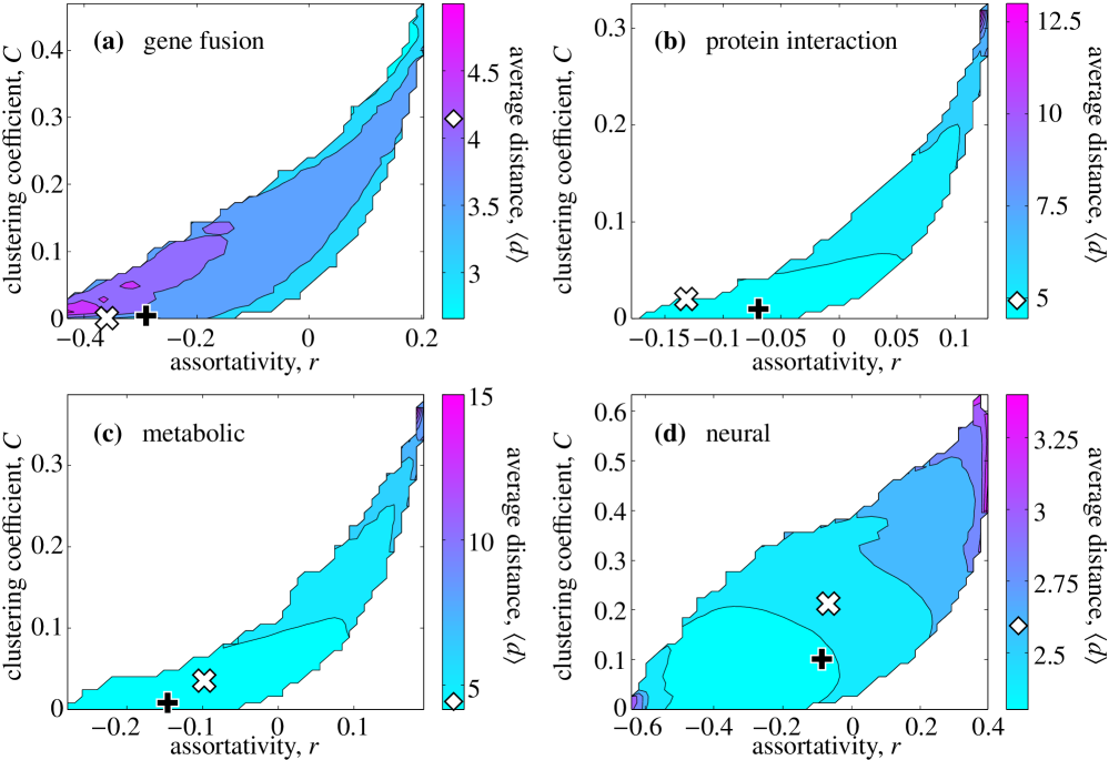
Figure 4: The average distance within the largest component $\langle d\rangle$ as a function of $r$ and $C$. The panes and symbols correspond to those of Fig. 3.

V.2 Distances in the largest component

In Fig. 4 we display the average distance in the largest component. As mentioned, measuring the distance can give complementary information to the $s(r,C)$ graphs of Fig. 3—while $s$ tells us how much of the network that can be reached, $\langle d\rangle$ tells us how fast that can happen. For all networks the big picture is that large connected components have large average distances. This is expected from most network models. There is, however, more information than this in Fig. 4: for components of the same size, the average distance is increasing with both $r$ and $C$. That $\langle d\rangle$ should increase with $C$ seems quite natural—if one of a triangle’s edges is rewired to connect two distant vertices, the distances in the surrounding of the triangle would increase with one, but this would be more than compensated by the connection of the two previously distant areas. Disassortative networks typically lack a well-defined core. Such cores are known to keep the average distance of general power-law networks short chung_lu:pnas . Thus one would expect an increase of $r$ to cause a larger $\langle d\rangle$, but apparently the clustering related length-increase outweighs this effect. In contrast to the relative size, the average distances of the real networks are close to the $\mathcal{G}(G)$-averages at the same $r$-$C$ coordinates. For the gene fusion network (with a relatively small largest component), this means the distances are rather large.

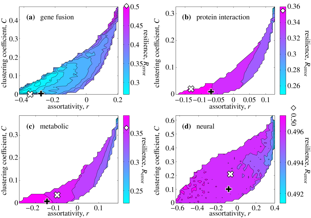
Figure 5: The error robustness $R_{\mathrm{error}}$ as a function of $r$ and $C$. The panes and symbols correspond to those of Fig. 3.

V.3 Error robustness

Next, we turn to the error robustness problem. As seen in Fig. 5 the gene fusion network (Fig. 5(a)), once again, has a qualitatively different behavior than the other three networks (Fig. 5(b), (c) and (d)). While the gene fusion network is most robust for high $r$- and $C$-values the other networks are most robust for low $r$. A sketchy explanation can be found in the chain-like subgraphs extending from the largest component in a large-$r$ network (cf. Fig. 2)—with a random deletion of vertices, these subgraphs are likely to be disconnected from the core rather soon (whereas in a disassortative network alternative paths may still exist), then if the deletion-robust core is less than half of the original component size it follows that it may soon be isolated. The sparsity of the gene fusion network makes the low-$r$ $\mathcal{G}(G)$-graphs much like trees (i.e., having few cycles), and since cycles provide redundant paths that can make a network robust, it follows that these graphs are fragile. For a fixed $r$, $R_{\mathrm{error}}$ is a decreasing function of $C$ for the three largest networks. We believe this is an effect of the local path redundancy induced by triangles—if one vertex of a triangle is deleted, the other two are still connected.

The $R_{\mathrm{error}}$-values for the real networks are always markedly higher than the $\mathcal{G}(G)$-averages for the same $(r,C)$-coordinates. Networks with highly skewed degree distributions (the gene fusion, protein interaction and metabolic networks) are known to be robust to errors by virtue of degree distribution alone alb:attack , now Fig. 5 tells us that all these networks have a yet higher error tolerance which is an indication that error robustness is an important factor in the evolution of these networks.

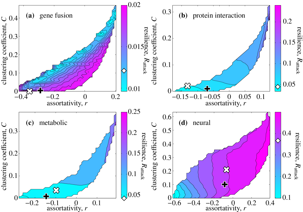
Figure 6: The error robustness $R_{\mathrm{attack}}$ as a function of $r$ and $C$. The panes and symbols correspond to those of Fig. 3.

V.4 Attack robustness

The final quantity we measure is the attack robustness (see Fig. 6). $R_{\mathrm{attack}}$’s functional dependence on $r$ and $C$ is quite different from that of $R_{\mathrm{error}}$. The gene fusion $\mathcal{G}(G)$ has the highest attack robustness at high $r$- and low $C$-values. The other networks have higher robustness values for high assortativity, but no clear tendency in the $C$-direction. The attack mechanism we study targets the high degree vertices. Having all high degree vertices connected to each other is probably the only way to keep the network from instantaneous fragmentation. The observed $r$-dependence is thus rather expected. The real-world networks all have $R_{\mathrm{attack}}$-values of the same order of magnitude as the average values for the $\mathcal{G}(G)$ networks of the same location in $r$-$C$ space. We note that for studying the attack problem of metabolic networks, the (less common) enzyme centric graph representation is more appropriate (see Sect. IV.2). The reason being that one can suppress an enzyme much easier than removing the substrates.

Table 2: Summary of the network structural measures of the real world networks relative to the average values of the $\mathcal{G}(G)$ a distance $\delta<0.02$ from the real network. “$<$” indicates that the real network have a lower value than the corresponding $\mathcal{G}(G)$-value. All results are significant with p-values $>0.01$, except the $s$-value of the neural network that has a p-value of $\sim 0.05$.

	gene fusion	protein interaction	metabolic	neural
$s$	$<$	$<$	$<$	$>$
$\langle d\rangle$	$<$	$<$	$<$	$<$
$R_{\mathrm{error}}$	$>$	$>$	$>$	$>$
$R_{\mathrm{attack}}$	$>$	$>$	$>$	$>$

V.5 Comparison between the graphs

Even though all our example networks are constructed from biological data, they represent fundamentally different systems—the neural network is spatial by nature, the protein interaction and (even more so) the metabolic networks are the background topology for an active dynamic system, whereas the gene fusion network is a representation of possible but undesired events. The protein interaction, metabolic and neural networks have one thing in common—the organism needs them to be robust to errors (caused by injuries, mutations, disease etc.) wagner:robu . As mentioned above and summarized in Table LABEL:tab:pval the error robustness is indeed higher for the real networks than the $\mathcal{G}(G)$-ensemble at the same $(r,C)$-coordinates. As mentioned above, the attack robustness of the real network is of the same order as the $\mathcal{G}(G)$-average at the same $(r,C)$-coordinate, but actually there is a significant tendency that these network also are more robust to attacks. Furthermore, the distances in the largest component, and the relative sizes $s$ are (with the neural network $s$-value as the only exception) smaller in the real than the $\mathcal{G}(G)$ networks.

Despite these similarities between the statistics of the real-world networks the $r$-$C$ space of the different degree sequences have qualitatively different network structure. Especially, the gene fusion network behaves almost the opposite of the other networks (at least for $s$, $\langle d\rangle$ and $R_{\mathrm{error}}$). The source of this opposite behavior (as we discuss above) is probably that it is much sparser than the other networks. The neural network is the densest network and the only one that do not have a power-law like degree distribution.

VI Discussion

Many complex network studies use the ensemble $\mathcal{G}(G)$ of graphs with the same degree sequence as the subject graph $G$ as a null model. In contrast to a generative network model, with a few degrees of freedom that has to be fitted approximately, such an ensemble has $O(N)$ degrees of freedom that can be matched exactly with the values of $G$. We argue that $\mathcal{G}(G)$ is more than a null model—by resolving the graphs of $\mathcal{G}(G)$ in a space defined by some network-structural measures, one can get a picture of the opportunities and limits there are (or has been) in the evolution of $G$. In this work we map out $\mathcal{G}(G)$ in the two-dimensional space defined by the clustering coefficient and the assortativity. Then we measure other network structural quantities throughout this space. One formal way to see our method is that we resolve $\mathcal{G}(G)$ in the (high dimensional) space of all sensible network measures. Then, for simplicity, we project to a few dimensions. (The case of projection to one dimension has been studied in a less formalized way earlier—projection to assortativity zj:spectrum or a “hierarchy” measure rosv:mountain .) An interesting open question is to find the principal components of the space of all sensible network measures. Using four example networks from biology, we measure average values of four network-structural quantities over the $r$-$C$ space and compare these with the values of the real networks.

The functional characteristics of the $r$-$C$ spaces varies much between the four example networks. For example, the C. elegans neural network covers a much larger area of the $r$-$C$ space, something that probably relates to its more narrow degree distribution. The human gene fusion network, on the other hand, has a broad degree distribution similar to the S. cerevisiae protein interaction and human metabolic networks, still the structural dependency on $r$ and $C$ is very different for the gene fusion network compared to the others. We argue that this difference stems from the sparseness of the gene fusion network. To achieve a comprehensive understanding about how the network structure throughout the $r$-$C$ space depends on the degree sequence, one would need a systematic investigation of different artificial degree sequences. In this paper, we do not pursue this goal beyond the analysis of the four biological data sets. The position of the real networks in the valid region of the $r$-$C$ space adds some further information. For example, it may have been the case that networks with lower assortativity have been favored during the evolution of the gene fusion network. Clustering, on the other hand, has probably not put any constraint on the network evolution. Furthermore we compare the network structure of the real networks with the average values of networks in $\mathcal{G}(G)$ that are close to the $(r,C)$-coordinates of the real network. From this analysis, we conclude that all our four example networks are more robust to both random errors and targeted attacks than what can be expected from a random network constrained to the same degree distribution, assortativity and clustering coefficient. For all networks, except maybe the gene fusion network, this is in line with robustness being an important factor in the network evolution. Note that in this work we assume the subject network to be accurate. To get more valid error estimates one would need to take the accuracy of the edges into account.

The analysis scheme presented in this paper can be further extended and analyzed. As mentioned, it would be interesting with a quantitative evaluation of the network-structural spaces, and how they depend on the degree sequence. One can also try, for time-resolved data sets, to incorporate dynamic information in the analysis by monitoring the network-evolutionary trajectory in the $r$-$C$ space.

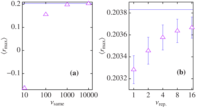
Figure 7: Convergence of the optimization algorithm. (a) shows the average maximal assortativity $\langle r_{\mathrm{max}}\rangle$ with $\nu_{\mathrm{rep.}}=1$. The horizontal line represents the result of the maximization algorithm of Ref. doyle:big . (b) shows the further improvement by finding the maximum over many independent runs (for $\nu_{\mathrm{same}}=10000$). The vertical bars indicates the standard deviation of the observed maxima.

Appendix A Convergence and sampling uniformity

In this Appendix, we address some technical issues of our method related to the convergence of our optimization algorithm and uniformity of the sampling. We will also motivate our choice of parameters.

A.1 Assortativity and clustering extremes

To find the extremal assortativity values we use the edge-swapping algorithm described in Sect. III. To find $r_{\mathrm{min}}$ we start from a random member of $\mathcal{G}(G)$ and swap random edge-pairs (keeping the graph simple at all times) that lower $r$. When no graph of lower $r$ has been found for $\nu_{\mathrm{same}}$ time steps, we break the iteration. To avoid the effect of being trapped in local minima, this process is repeated $\nu_{\mathrm{rep.}}$ times. The main motivation for using this method is that it is at heart the same scheme as for obtaining the extremal clustering values and sampling the valid region (and thus we can re-use the same code for many steps of the calculations). In this section, we argue that the optimization performance of this method is sufficiently good for our purpose.

There is a deterministic method to maximize the assortativity that is, if it exits properly, guaranteed to find $r_{\mathrm{max}}$ doyle:big . The method works as follows: First all vertex-pairs $(i,j)$ are ranked in decreasing order of the product of their degrees, $k_{i}k_{j}$. Then the edges are added in order of this list unless the degree of one of the vertices already is fulfilled. There are some other technicalities from the additional constraint (of the authors) that the network should be connected. Of our networks, only the neural network has such an evolutionary constraint, so we do not impose it.

In Fig. 7 we display the parameter dependence of the convergence for the gene fusion network. The horizontal line is the theoretical maximum obtained by the algorithm of Ref. doyle:big . When $\nu_{\mathrm{same}}=10000$ we obtain an average maximal assortativity within $0.001$ of the theoretical maximum (Fig. 7(a)). By increasing $\nu_{\mathrm{rep.}}$ the accuracy can be increased further (Fig. 7(b)). The lattice spacing we use is $0.005\lesssim r\lesssim 0.02$, so we deem a precision of $0.001$ sufficient. The gene fusion network is our smallest network but the other networks are not harder to converge. When one edge-pair is swapped so that $r$ decreases, the only term of Eq. 1 that changes is $\langle k_{1}\,k_{2}\rangle$. The potential change of the sum $\sum_{(i,j)\in E}k_{i}k_{j}$, in the calculation of $\langle k_{1}\,k_{2}\rangle$ (close to the extrema) is of the order of the typical degree values of the network. These values grow slower than the network itself, which means that a larger network can be closer in $r$, but further away in number of edge swaps to reach the global optimum, than a smaller network. Some authors doyle:big use $\sum_{(i,j)\in E}k_{i}k_{j}$ to measure the degree correlations, but since we strive for a macroscopic level of description (consistent in the large-$N$ limit), $r$ is a more appropriate quantity for the present work.

The optimization of the clustering to find the minima (maxima) of the segments of assortativity space follows the same pattern as the method to find the minimal (maximal) $r$. Changes of the parameters ($\nu_{\mathrm{same}}$ and $\nu_{\mathrm{rep.}}$) have the same effect as in Fig. 7, and the same values seem sufficient.

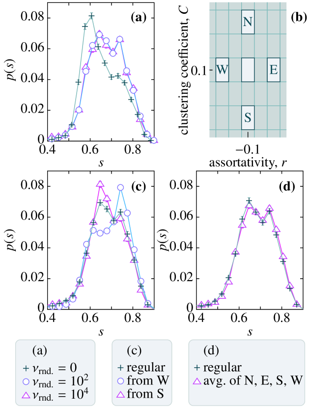
Figure 8: Histograms of $s$ for the discussion of sampling uniformity. All the histograms are from the gene fusion network and a pixel centered around $r=-0.1$, $C=0.1$ (the dimensions of a pixel is $\Delta r=0.013$, $\Delta C=0.0096$. The error bars represent standard errors. Lines are guides for the eyes. (a) shows the histograms with a different numbers of random edge-pair swappings $\nu_{\mathrm{rnd.}}$ within the pixel before the measurements of quantities. (b) illustrates the location of the starting point pixels used in panels (c) and (d). (c) compares histograms for swapping processes starting at W, S with the regular algorithm. (d) compares the average histogram of walks starting in the four peripheral points of (b) with the result of the regular algorithm. In panels (c) and (d) $\nu_{\mathrm{rnd.}}=1000$. The whole range of the histograms is not shown, which is why the areas under the curves appear different.

A.2 Sampling uniformity

The other technical issue we address in this Appendix is the uniformity of our sampling procedure. Ideally we would like all unique (i.e., non-isomorphic) members of $\mathcal{G}(G)$ to be sampled with the same probability. The most important observation is trivial—by edge-pair swapping one can go from one member of $\mathcal{G}(G)$ to any other, and thus all members of the ensemble will contribute to the averages. A much harder question is whether or not every member of $\mathcal{G}(G)$ is sampled with uniform probability. In this section, we will argue that our algorithm does a reasonably good job in the sense that there are no inconsistencies and parameter values are appropriate.

When the target pixel is found (step 15 of the algorithm) we perform $\nu_{\mathrm{rnd.}}$ additional random edge-pair swaps. The idea is to sample the $\mathcal{G}(G)$-members of the pixel more uniformly (and indeed to be able to reach into the interior of the pixel). In Fig. 8(a) we illustrate the effect of these random moves. We plot a normalized histogram of the relative largest cluster size $s$ for $0$, $100$ and $10000$ random moves. We see that these moves do make a difference (the $\nu_{\mathrm{rnd.}}=0$ is different from the $\nu_{\mathrm{rnd.}}=100$) but it does not matter if $\nu_{\mathrm{rnd.}}=100$ or $\nu_{\mathrm{rnd.}}=10000$. The same situation is observed for other pixels, networks and quantities. Therefore, we use $\nu_{\mathrm{rnd.}}=1000$ in this work.

Next, we will illustrate the use of the randomly permuted list in the sampling of the pixels (steps 11 and 12 of the algorithm). The motivation for this procedure is that the network structure can depend on the direction from which the search arrives to the pixel. In Fig. 8(b) we illustrate the test procedure—we sample separate histograms from four starting points in the four cardinal directions with respect to the central $(r,C)=(-0.1,0.1)$ pixel. In Fig. 8(c) we see that the histograms from the W and S pixels are different. There appears to be two regions of $\mathcal{G}(G)$ contributing to these histograms (one with $s\approx 0.65$, one with $s\approx 0.75$). Searches starting from W seem to arrive at the $s\approx 0.75$ region more frequently, and searches staring at S ends up around $s\approx 0.65$ more frequently. The curve of the actual algorithm weighs the two peaks more equal. The curves from N and E coincides almost completely the curve for the regular algorithm (and are therefore omitted for clarity). The impression we get is that the search from one direction can induce a bias in the network structure (symbolically speaking, the graphs have a preference for ending up in a certain region of $\mathcal{G}(G)$). However, from other directions, or by the random sampling of pixels (step 11), the bias is reduced. This picture is further strengthened in Fig. 8(d) where we show that the average value of the histograms from the four starting points are overlapping with the histogram of the regular algorithm.

References

- (1) R. Albert and A.-L. Barabási. Statistical mechanics of complex networks. Rev. Mod. Phys, 74:47–98, 2002.
- (2) R. Albert, H. Jeong, and A.-L. Barabási. Attack and error tolerance of complex networks. Nature, 406:378–382, 2000.
- (3) L. A. N. Amaral, A. Scala, M. Barthélémy, and H. E. Stanley. Classes of small-world networks. Proc. Natl. Acad. Sci. USA, 97:11149–11152, 2000.
- (4) J. B. Axelsen, S. Bernhardsson, M. Rosvall, K. Sneppen, and A. Trusina. Degree landscapes in scale-free networks. Phys. Rev. E, 74:036119, 2006.
- (5) A.-L. Barabási and R. Albert. Emergence of scaling in random networks. Science, 286:509–512, 1999.
- (6) A. Barrat and M. Weigt. On the properties of small-world network models. Eur. Phys. J. B, 13:547–560, 2000.
- (7) F. Chung and L. Lu. The average distances in random graphs with given expected degrees. Proc. Natl. Acad. Sci. USA, 99:15879–15882, 2002.
- (8) S. N. Dorogovtsev and J. F. F. Mendes. Evolution of Networks: From Biological Nets to the Internet and WWW. Oxford University Press, Oxford, 2003.
- (9) P. Erdős and A. Rényi. On random graphs I. Publ. Math. Debrecen, 6:290–297, 1959.
- (10) D. Gale. A theorem of flows in networks. Pacific J. Math., 7:1073–1082, 1957.
- (11) M. Höglund, A. Frigyesi, and F. Mitelman. A gene fusion network in human neoplasia. Oncogene, 25:2674–2678, 2006.
- (12) P. W. Holland and S. Leinhardt. Some evidence on the transitivity of positive interpersonal sentiment. Am. J. Sociol., 72:1205–1209, 1972.
- (13) P. Holme and M. Huss. Role-similarity based functional prediction in networked systems: application to the yeast proteome. J. Roy. Soc. Interface, 2:327–333, 2005.
- (14) P. Holme, B. J. Kim, C. N. Yoon, and S. K. Han. Attack vulnerability of complex networks. Phys. Rev. E, 65:066109, 2002.
- (15) M. Huss and P. Holme. Currency and commodity metabolites: Their identification and relation to the modularity of metabolic networks. e-print q-bio/0603038.
- (16) L. Katz and J. H. Powell. Probability distributions of random variables associated with a structure of the sample space of sociometric investigations. Ann. Math. Stat., 28:442–448, 1957.
- (17) V. Latora and M. Marchiori. Efficient behavior of small-world networks. Phys. Rev. Lett., 87:198701, 2001.
- (18) L. Li, D. Alderson, J. C. Doyle, and W. Willinger. Towards a theory of scale-free graphs: Definition, properties, and implications. Internet Mathematics, 2:431–523, 2005.
- (19) S. Maslov and K. Sneppen. Specificity and stability in topology of protein networks. Science, 296:910–913, 2002.
- (20) S. Maslov, K. Sneppen, and A. Zaliznyak. Detection of topological patterns in complex networks: Correlation profile of the Internet. Physica A, 333:529–540, 2004.
- (21) F. Mitelman, B. Johansson, and F. Mertens. Fusion genes and rearranged genes as a linear function of chromosome aberrations in cancer. Nature Genetics, 36:331–334, 2004.
- (22) A. E. Motter. Cascade control and defense in complex networks. Phys. Rev. Lett., 93:098701, 2004.
- (23) M. E. J. Newman. Assortative mixing in networks. Phys. Rev. Lett., 89:208701, 2002.
- (24) M. E. J. Newman. The structure and function of complex networks. SIAM Review, 45:167–256, 2003.
- (25) M. E. J. Newman and J. Park. Why social networks are different from other types of networks. Phys. Rev. E, 68:036122, 2003.
- (26) S. Shen-Orr, R. Milo, S. Mangan, and U. Alon. Network motifs in the transcriptional regulation network of Escherichia coli. Nature Genetics, 31:64–68, 2002.
- (27) O. Sporns, G. Tononi, and G. M. Edelman. Theoretical neuroanatomy: Relating anatomical and functional connectivity in graphs and cortical connection matrices. Cerebral Cortex, 10:127–141, 2000.
- (28) A. Wagner. Robustness and Evolvability in Living Systems. Princeton University Press, Princeton NJ, 2005.
- (29) L. R. Walker and R. E. Walstedt. Computer model of metallic spin-glasses. Phys. Rev. B, 22:3816–3842, 1980.
- (30) S. Wasserman and K. Faust. Social network analysis: Methods and applications. Cambridge University Press, Cambridge, 1994.
- (31) J. G. White, E. Southgate, J. N. Thompson, and S. Brenner. The structure of the nervous system of the nematode C. Elegans. Philos. Trans. Roy. Soc. Lond., 314:1–340, 1986.
- (32) J. Zhao, L. Tao, H. Yu, J.-H. Luo, Z.-W. Cao, and Y.-X. Li. The spectrum of degree correlations: topological diversity of networks with a given degree sequence. e-print cond-mat/0611104.
- (33) J. Zhao, H. Yu, J. Luo, Z. W. Cao, and Y.-X. Li. Complex networks theory for analyzing metabolic networks. Chinese Science Bulletin, 51:1529–1537, 2006.