Mutation, selection, and ancestry in branching models: a variational approach

Abstract

We consider the evolution of populations under the joint action of mutation and differential reproduction, or selection. The population is modelled as a finite-type Markov branching process in continuous time, and the associated genealogical tree is viewed both in the forward and the backward direction of time. The stationary type distribution of the reversed process, the so-called ancestral distribution, turns out as a key for the study of mutation-selection balance. This balance can be expressed in the form of a variational principle that quantifies the respective roles of reproduction and mutation for any possible type distribution. It shows that the mean growth rate of the population results from a competition for a maximal long-term growth rate, as given by the difference between the current mean reproduction rate, and an asymptotic decay rate related to the mutation process; this tradeoff is won by the ancestral distribution.

We then focus on the case when the type is determined by a sequence of letters (like nucleotides or matches/mismatches relative to a reference sequence), and we ask how much of the above competition can still be seen by observing only the letter composition (as given by the frequencies of the various letters within the sequence).

If mutation and reproduction rates can be approximated in a smooth way, the fitness of letter compositions resulting from the interplay of reproduction and mutation is determined in the limit as the number of sequence sites tends to infinity.

Our main application is the quasispecies model of sequence evolution with mutation coupled to reproduction but independent across sites, and a fitness function that is invariant under permutation of sites. In this model, the fitness of letter compositions is worked out explicitly. In certain cases, their competition leads to a phase transition.

1 Introduction

Evolution is often understood as an optimization process of some kind, and there is a long tradition to consider evolutionary models, particularly those from population genetics, from a variational perspective. The most popular result in this context is known as the Fundamental Theorem of Natural Selection (FTNS). In its simplest form it states that, in the deterministic selection equation for a single locus in continuous time, mean fitness can only increase along trajectories (i.e., it is a Lyapunov function), and the rate of this increase equals the variance in fitness, cf. [5, Ch. I.10.3]. More sophisticated versions in the context of quantitative genetics and multiple loci, along with a general discussion of optimality principles for the selection equation, are discussed in [5, Ch. II.6.3–II.6.6] and [11, Ch. 2.9, 7.4.5 and 7.4.6]; see also [8].

If, rather than selection alone, the joint dynamics of selection and mutation is considered, results become sparse. The FTNS may be generalized to house-of-cards mutation (i.e., mutation rates are independent of the parent type), see [1] and [19]. If mutation is reversible, a Lyapunov function is available for a certain $L^{2}$-renormalized version of the dynamics, but not for the original mutation-selection equation [33].

The above approaches refer to the genetic (or, more generally, type) composition at the population level. In contrast, this article is concerned with a variational principle in mutation-selection models (and closely related branching processes) from the point of view of individual lineages through time, their ancestry and genealogy. This principle is related to the (stochastic) processes that take place along such lines of descent, with a special emphasis on the relation between the present and the past. We will, however, not include genetic drift (i.e., resampling) into our models; therefore, our backward point of view differs from that of the coalescent process (see [17] for a recent review of this area).

The paper is organized as follows. In Section 2, we will set up our model(s) and recapitulate a few fundamental facts. Section 3 provides an informal preview of the results that will be detailed (and proved) in the remainder of the article. Section 4 will develop the lineage aspect that will be required furtheron. Looking at the mutation process along individual lines, we will obtain a fairly general variational principle (Section 5, Thm. 5.1), which quantifies the tradeoff between the mean reproduction rate along a line and the asymptotic rate at which it is lost; it further implies a connection between the type processes that emerge in the forward and backward directions of time. In Sections 6 and 7, we will specialize on the case where types are sequences over a finite alphabet. If mutation is independent and fitness is additive across sites, the original high-dimensional variational principle may be reduced to a simpler, low-dimensional one (Section 6.3, Thm. 6.1). The same holds asymptotically if mutation rates and fitness function allow for a suitable smooth approximation when the number of sites gets large (Section 7, Thms. 7.1, 7.2 and 7.3). The corresponding approximate maximum principle will be derived explicitly for the quasispecies model of sequence evolution (Section 8, Thm. 8.1).

The paper ties together, unifies and generalizes various aspects that have appeared in previous publications. Special cases of the low-dimensional maximum principle were first described in [18], and applied to concrete examples. An extension appeared in [3]; it relies on methods from linear algebra and asymptotic analysis, but makes no connection to the stochastic processes on individual lines, nor does it include worked examples. The connection to the backward point of view relies on earlier work on branching processes [22, 23] and was investigated in [18] and [15]. These results will reappear here as parts of a larger picture.

2 Models and basic facts

2.1 Models

Consider a finite set of types $S$ (with $|S|>1$) and a population of individuals, each of which carries one of these types. (We think of individuals as haploid, and of types as alleles.)

2.1.1 The parallel mutation-reproduction model. Let us start with the most basic mutation-reproduction model in which mutation and reproduction occur in parallel, that is, independently. As depicted in Fig. 1,

\psfrag{D}{$D_{i}$}\psfrag{B}{$B_{i}$}\psfrag{i}{$i$}\psfrag{j}{$j$}\psfrag{U}{$U_{ij}$}\includegraphics{museP.eps}

Figure 1: The parallel mutation-reproduction model.

an individual of type $i\in S$ may, at every instant in continuous time, do either of three things: It may split, i.e., produce a copy of itself (this happens at birth rate $B_{i}\geq 0$), it may die (at rate $D_{i}\geq 0$), or it may mutate to type $j\;(j\neq i)$ (at rate $U_{ij}\geq 0$). Different meanings may be associated with this verbal description. Probabilists will take it to mean a multi-type Markov branching process in continuous time (see [2, Ch. V.7], or [25, Ch. 8] for a general overview). That is, an $i$-individual waits for an exponential time with parameter $A_{i}=B_{i}+D_{i}+\sum_{j:j\neq i}U_{ij}$, and then dies, splits or mutates to type $j\neq i$ with probabilities $B_{i}/A_{i},D_{i}/A_{i}$, and $U_{ij}/A_{i}$, respectively. The number of individuals of type $j$ at time $t$, $Z_{j}(t)\in\mathbb{Z}_{\geq 0}:=\{0,1,2\dots\}$, is a random variable; the collection $Z(t)=\big{(}Z_{j}(t)\big{)}_{j\in S}$ is a random vector. The corresponding expectation is described by the first-moment generator $\boldsymbol{A}=\boldsymbol{U}+\boldsymbol{R}$. Here, $\boldsymbol{U}$ is the Markov generator $\boldsymbol{U}=(U_{ij})_{i,j\in S}$, where the mutation rates $U_{ij}$ for $j\neq i$ are complemented by $U_{ii}:=-\sum_{j:j\neq i}U_{ij}$ for all $i\in S$. Further, $\boldsymbol{R}:=\mbox{diag}\{R_{i}\mid i\in S\}$, where $R_{i}:=B_{i}-D_{i}$ is the net reproduction rate (or Malthusian fitness). More precisely, we have $\mathbb{E}^{i}(Z_{j}(t))=({\rm e}^{t\boldsymbol{A}})_{ij}$, where $\mathbb{E}^{i}(Z_{j}(t))$ is the expected number of $j$ individuals at time $t$ in a population started by a single $i$-individual at time $0$.

2.1.2 Deterministic aspects. Ignoring stochastic effects and focussing on the mean behaviour of the population, one often considers the deterministic mutation-reproduction model

$$\dot{y}(t)=y(t)\boldsymbol{A},\qquad y(0)=y_{0},$$ (1)

where $y(t)=(y_{i}(t))_{i\in S}$ is the row vector associating to each type $i$ its abundance $y_{i}(t)\in\mathbb{R}_{\geq 0}$ (i.e., the size of the subpopulation of type $i$). As $y(t)=y_{0}{\rm e}^{t\boldsymbol{A}}$, the deterministic model describes the expectation of the corresponding branching process, provided the initial condition is chosen accordingly.

However, the independent reproduction of individuals as implied so far is unrealistic for large populations. They usually experience density regulation; in the simplest case, this is modelled by an additional death term $\gamma(t)\geq 0$, that is, $D_{i}$ is replaced by $D_{i}+\gamma(t)$ (for all $i\in S$), where $\gamma(t)$ may depend on time (maybe through total population size), but not on the type. Then, of course, (1) generalizes to

$$\dot{y}(t)=y(t)(\boldsymbol{A}-\gamma(t)\boldsymbol{I}),$$ (2)

where $\boldsymbol{I}$ is the identity matrix. In theoretical ecology, a wide variety of models is in use that specify $\gamma$ for the many biological situations that may arise. In population genetics, however, one is usually more interested in the relative frequencies $q_{i}(t):=y_{i}(t)/\sum_{j}y_{j}(t)$. Differentiating this and inserting (2) leads to

$$\dot{q}_{i}(t)=q_{i}(t)\left(R_{i}-\langle q(t),R\rangle\right)+\sum_{\begin{subarray}{c}j\in S:\\ j\neq i\end{subarray}}\big{(}q_{j}(t)U_{ji}-q_{i}(t)U_{ij}\big{)},$$ (3)

independently of $\gamma$. Here we think of the row vector $q=(q_{i})_{i\in S}$ as a probability measure, of the column vector $R=(R_{i})_{i\in S}$ as a function on $S$ (known as the fitness function), and of the scalar product $\langle q(t),R\rangle=\sum_{i\in S}q_{i}(t)R_{i}$ as the associated expectation, namely, the mean fitness of the population at time $t$. Eq. (3) is the well-known parallel (or decoupled) mutation–selection model, which goes back to [6, p. 265]. Although we have derived it here for haploid populations (and will adhere to this picture), it is well known, and easily verified, that the same equation describes diploids without dominance (in an approximation using Hardy-Weinberg proportions). For a comprehensive review of the model and its properties, see [5, Ch. III].

Rather than considering deterministic and stochastic models separately, we aim at a unifying picture and note that the branching process is particularly versatile: Its expectation fulfills (1), and the solution of (1), in turn, implies that of (3) (via normalization). Properties of the branching process will, therefore, immediately translate into properties of the mutation-selection equation (but not, necessarily, vice versa). For this reason, we will consider the branching process as our primary model throughout this paper. Let us, therefore, return to branching populations and look at alternatives to the parallel model.

2.1.3 The coupled mutation-reproduction model. In this model one assumes that mutations occur on the occasion of reproduction events (see Fig. 2): An $i$-individual again dies at rate $D_{i}$ and gives birth at rate $B_{i}$, but every time it gives birth, the offspring is possibly mutated (of type $j$ with probability $P_{ij}$), while the parent itself survives unchanged. The corresponding first-moment generator $\boldsymbol{A}$ has elements

$$A_{ij}=B_{i}P_{ij}-D_{j}.$$ (4)

An example of the coupled model will be studied in Sec. 8.

\psfrag{D}{$D_{i}$}\psfrag{BP}{$B_{i}P_{ij}$}\psfrag{i}{$i$}\psfrag{j}{$j$}\includegraphics{museC.eps}

Figure 2: The coupled mutation-reproduction model.

2.1.4 General splitting rules. Both the parallel and the coupled models are special cases of the general Markov branching model as depicted in Fig. 3: An $i$-individual lives for an exponential time $\tau_{i}$ with prescribed parameter $A_{i}$ and then produces a random offspring $N_{i}=(N_{ij})_{j\in S}$ with distribution $\boldsymbol{p}_{i}$ on $\mathbb{Z}_{+}^{S}$ and finite means $\mathbb{E}(N_{ij})$ for all $i,j\in S$. More precisely, $N_{ij}\in\mathbb{Z}_{\geq 0}$ is the number of children of type $j$, and $\boldsymbol{p}_{i}(\kappa)=\mathbb{P}(N_{ij}=\kappa_{j}\,,\forall j\in S)$. The first-moment generator $\boldsymbol{A}$ has elements $A_{ij}=A_{i}(\mathbb{E}(N_{ij})-\delta_{ij})$.

\psfrag{i}{$i$}\psfrag{underbrace}{$\underbrace{\mbox{\hskip 80.00012pt}}_{\textstyle\tau_{i}}$}\psfrag{Nij}{\raisebox{2.15277pt}{\mbox{\large$\Bigg{\}}$}} $\,N_{i}=(N_{ij})_{j\in S}$}\includegraphics{general.eps}

Figure 3: General splitting rules.

For the coupled and the general branching rules, the first-moment generator may again be written in the ‘parallel’ form $\boldsymbol{A}=\boldsymbol{U}+\boldsymbol{R}$ where $\boldsymbol{U}$ is a Markov generator and $\boldsymbol{R}$ is a diagonal matrix; this decomposition is uniquely given by $U_{ij}=A_{ij}\mbox{ for }i\neq j$, $U_{ii}=-\sum_{j:j\neq i}U_{ij}$, and $R_{i}=\sum_{j\in S}A_{ij}$ for all $i\in S$. At the time being, this is a formal decomposition, but will receive its branching process interpretation later in Sec. 4.2. The corresponding deterministic models then all take the form (1) and (3), provided the parameters are interpreted in the above way.

2.2 Fundamental facts

2.2.1 Forward view and long-time characteristics. We will assume throughout that $\boldsymbol{A}$ (or, equivalently, $\boldsymbol{U}$) is irreducible. Perron-Frobenius theory then tells us that $\boldsymbol{A}$ has a principal eigenvalue $\lambda$ (namely a real eigenvalue exceeding the real parts of all other eigenvalues) and associated positive left and right eigenvectors $\pi$ and $h$ which will be normalized so that $\langle\pi,\mathsf{1}\rangle=1=\langle\pi,h\rangle$, where $\mathsf{1}=(1)_{i\in S}$ is the vector with all coordinates equal to $1$. We will further assume that $\lambda>0$, i.e., the branching process is supercritical. This implies that the population will, in expectation, grow in the long run, as is obvious from (1); in individual realizations, it will survive with positive probability, and then grow to infinite size with probability one, see (6) below.

The asymptotic properties of our models forward in time are, to a large extent, determined by $\lambda,\pi$, and $h$, and provide further connections between the stochastic and the deterministic pictures. The left eigenvector $\pi$ holds the stationary composition of the population, in the sense that $\lim_{t\to\infty}q(t)=\pi$ for the differential equation (3), and, for the branching process,

$$\lim_{t\to\infty}\frac{Z(t)}{\|Z(t)\|_{1}}=\pi\quad\text{with probability one, conditionally on survival},$$ (5)

where $\|Z(t)\|_{1}:=\sum_{j\in S}Z_{j}(t)$ is the total population size. This is due to the famous Kesten-Stigum theorem, see [27] for the discrete-time original, and [2, Thm. 2, p. 206] and [15, Thm. 2.1] for continuous-time versions. Furthermore,

$$\langle\pi,R\rangle=\lambda=\lim_{t\to\infty}\frac{1}{t}\log\|y(t)\|_{1}=\lim_{t\to\infty}\frac{1}{t}\log\|Z(t)\|_{1}$$ (6)

is the asymptotic growth rate (or equilibrium mean fitness) of the population. Here the first equality follows from the identity $\lambda=\langle\pi\boldsymbol{A},\mathsf{1}\rangle=\langle\pi,\boldsymbol{A}\mathsf{1}\rangle=\langle\pi,R\rangle$; the second one is an immediate consequence of (1) and Perron-Frobenius theory, and the third is from [15] and holds with probability one in the case of survival. Finally, the $i$-th coordinate $h_{i}$ of the right eigenvector $h$ measures the asymptotic mean offspring size of an $i$ individual, relative to the total size of the population:

$$h_{i}=\lim_{t\to\infty}\mathbb{E}^{i}\big{(}\|Z(t)\|_{1}\big{)}{\rm e}^{-\lambda t}.$$ (7)

For more details concerning this quantitity, see [18] and [15] (for the deterministic and stochastic pictures, respectively).

2.2.2 Backward view and ancestral distribution. In the above, we have adopted the traditional view on branching processes, which is forward in time. It is less customary, but equally rewarding, to look at branching populations backward in time. To this end, consider picking individuals randomly (with equal weight) from the current population and tracing their lines of descent backward in time (see Fig. 4). If we pick an individual at time $t$ and ask for the probability that the type of its ancestor is $i$ at an earlier time $t-\tau$, the answer will be $\alpha_{i}=\pi_{i}h_{i}$ in the limit when first $t\to\infty$ and then $\tau\to\infty$. Thus the distribution $\alpha=(\alpha_{i})_{i\in S}$ describes the population average of the ancestral types and is termed the ancestral distribution, see [15, Thm. 3.1] for details. Likewise, the time average along ancestral lines also converges to $\alpha$ in the long run, see [15, Thm. 3.2].

\psfrag{t}{$t$}\psfrag{ttau}{$t-\tau$}\includegraphics{backwardtree2.eps}

Figure 4: The backward point of view. The various types are indicated by different line styles. The fat lines mark the lines of descent defined by three individuals (bullets) picked from the branching population at time $t$. After coalescence of two such lines, the common ancestor receives twice the ‘weight’, as indicated by the extra fat line; this motivates the factor $h_{i}$ in the ancestral distribution.

If we pick individuals from the population at a very late time (so that its composition is given by the stationary vector $\pi$), then the type process in the backward direction is the Markov chain with generator $\bar{\boldsymbol{G}}=(\bar{G}_{ij})_{i,j\in S}$, $\bar{G}_{ij}=\pi_{j}(A_{ji}-\lambda\delta_{ij})\pi_{i}^{-1}$, as first identified by Jagers [22, 23]. The corresponding time-reversed process has generator $\boldsymbol{G}=(G_{ij})_{i,j\in S}$, where

$$G_{ij}=\alpha_{j}\bar{G}_{ji}\alpha_{i}^{-1}=h_{i}^{-1}(A_{ij}-\lambda\delta_{ij})h_{j};$$ (8)

it has been considered in [15], has been termed the retrospective process, and may be understood as the forward type process along the ancestral lines leading to typical individuals of the present population. By definition, $\boldsymbol{G}$ and $\bar{\boldsymbol{G}}$ both have stationary distribution $\alpha$.

3 Preview of results

In this Section, we will give an informal preview of the results that will be obtained in the remainder of the article. This overview will not aim at full generality, nor will it dwell on specific technical conditions that are required to make things precise. Rather, we will try and motivate the concepts and explain the results in the context of the model. The details will be worked out in the later Sections.

We will work our way from the more general to the more specific. We will start with a general variational principle, valid for all model variants of the previous Section, irrespective of the type space and of the parameters. Next, we will specialize on the case where types are sequences, and mutation and reproduction rates are invariant under permutation of sites. This will allow to dissect the variational problem into two simpler problems, which are easier to solve. Finally, we will treat one specific example, namely, the quasispecies model of sequence evolution, in full detail.

3.1 The general variational principle

A main object of this paper is to show that the asymptotic growth rate $\lambda$ of the population can be understood as the result of a competition between the mutation and reproduction processes along a typical ancestral line. In this informal Section, however, we will avoid the family tree picture, and rather imagine we are observing just one line. To start with, we even ignore reproduction, and consider only the simple Markov process $\{M(t)\}_{t\geq 0}$ on $S$ with generator $\boldsymbol{U}$; i.e., the type process which associates with $t$ the type at time $t$ under the mutation model $\boldsymbol{U}$. A crucial quantity in what follows will be the corresponding empirical measure

$$L(t):=\frac{1}{t}\int_{0}^{t}\delta_{M(\tau)}d\tau,$$ (9)

i.e., the random vector with components $L_{i}(t):=\frac{1}{t}\int_{0}^{t}\mathbb{I}\{M(\tau)=i\}d\tau$, where $\mathbb{I}\{.\}$ denotes the indicator function. This quantity measures the fraction of time the process spends in the various states, and hence is also known as occupation time measure. Clearly, $L(t)$ is a random element of $\mathsf{P}(S)$, the set of all probability measures on $S$. It is well-known by the ergodic theorem for Markov chains that, for $t\to\infty$, one has $L(t)\to\rho$ with probability one, where $\rho$ is the stationary distribution of $\boldsymbol{U}$. It is, perhaps, less well-known that the rate of convergence may be characterized asymptotically by a so-called large deviation principle, which may be informally put as

$$\mathbb{P}(L(t)\sim\nu)\approx{\rm e}^{-tI_{\boldsymbol{U}}(\nu)}\quad\text{for large}\;t,$$ (10)

that is, the probability that $L(t)$ is close to some measure $\nu$ decays exponentially, for large time, with a decay rate (or rate function) $I_{\boldsymbol{U}}(\nu)$ which can be written down explicitly (see (25) and (30) below). $I_{\boldsymbol{U}}$ is nonnegative, and $I_{\boldsymbol{U}}(\nu)=0$ precisely for $\nu=\rho$, in line with the above fact that, in the long run, only the stationary measure $\rho$ will survive.

Let us now add reproduction, i.e., turn to the branching process. As a consequence of the above large deviation principle, we will obtain, in Thm. 5.1, a link between the forward-time stationary distribution $\pi$ of the branching process, the reproduction rate $R$, the asymptotic growth rate $\lambda$, the mutation process $\boldsymbol{U}$ and the ancestral distribution $\alpha$, namely, the equation

$$\langle\pi,R\rangle=\lambda=\max_{\nu\in\mathsf{P}(S)}\big{[}\langle\nu,R\rangle-I_{\boldsymbol{U}}(\nu)\big{]}=\langle\alpha,R\rangle-I_{\boldsymbol{U}}(\alpha)\,.$$ (11)

This variational principle may be understood in terms of a competition between all possible distributions for a maximal long-term growth rate, as given by the difference between the current mean reproduction rate $\langle\nu,R\rangle$, and the asymptotic decay rate $I_{\boldsymbol{U}}(\nu)$. The first quantity is maximized by those measures that put mass only on the fittest type(s); the second one is minimized by $\rho$; the tradeoff is won by $\alpha$. Furthermore, (11) connects the forward and the retrospective point of view in that the maximum equals the mean fitness $\langle\pi,R\rangle$ of the stationary population. Note that the mean fitness of the ancestral population exceeds the mean fitness of the stationary one by $I_{\boldsymbol{U}}(\alpha)$, which is positive unless $\alpha=\rho$ (which implies $R_{i}=\text{const.}$, i.e., there is no selection). This reflects the fact that the present population carries with it a tail of (mainly unfavourable) mutants that are present at any time, but do not survive in the long run.

We will see in Sec. 5 that this ‘competition of distributions’ can be made more concrete, namely, in terms of a competition of lines of descent, by considering the empirical distributions $L^{\omega}(t)$ of types along distinct lines $\omega$. But before we can embark on this, we must first develop a way of constructing trees, lines, and processes on lines, in a consistent way; this will be taken up in the next Section.

It is interesting to note that the above variational principle resembles the thermodynamic maximum principles in statistical physics. Indeed, our reproduction rates may be identified with an energy, and the rate function with an entropy; in fact, the rate function for the continuous-time Markov chain $M(t)$ can be naturally derived from the usual entropy governing the so-called pair-empirical measure of a discrete-time Markov chain, cf. [20, Ch. IV].

3.2 Sequence space models

The variational principle (11), valuable as it is conceptually, is not very useful if one aims at an explicit solution; this is because maximization is over a large space (the set of probability measures on $S$). However, it turns out that, in certain models of sequence evolution, this task boils down to a much simpler one if the original problem is dissected into two, one of which can be solved explicitly. Let us first describe this ‘divide and conquer’ strategy.

Assume that the type of an individual is characterized by a sequence of nucleotides, amino acids, matches/mismatches with respect to a reference sequence of nucleotides, or, in general, letters from some alphabet $\varSigma$. Thus $\varSigma=\{A,G,C,T\}$, $\{1,\ldots,20\}$, $\{0,1\}$, or any other finite set. The natural type space is then $\varSigma^{N}$, the set of possible sequences of length $N$, where $N$ is typically large. However, if the mutation and reproduction rates are invariant under permutations of sequence sites, all relevant information on a sequence $\sigma=(\sigma_{k})_{1\leq k\leq N}\in\varSigma^{N}$ is already contained in its letter histogram (or letter composition)

$$H(\sigma)=(H_{\ell}(\sigma))_{\ell\in\varSigma}\,,\quad H_{\ell}(\sigma)=\sum_{k=1}^{N}\mathbb{I}\{\sigma_{k}=\ell\},$$ (12)

which indicates how often each letter $\ell$ shows up in $\sigma$. In other words, it is sufficient to look at the reduced type space

$$S=H(\varSigma^{N})=\Big{\{}i\in\mathbb{Z}^{d}\mid i_{\ell}\geq 0\>\text{for}\>\ell\in\varSigma,\;\sum_{\ell\in\varSigma}i_{\ell}=N\Big{\}},$$ (13)

with $d=\lvert\varSigma\rvert$, which consists of all possible letter compositions.

$$\text{\normalsize$\varSigma^{N}$}\stackrel{{\scriptstyle\text{\small$H$}}}{{\text{\Large$\longrightarrow$}}}\text{\normalsize$S$}$$

Figure 5: Lumping a sequence space.

This lumping procedure induces a model on $S$ that is again a Markov branching process; its reproduction rates $R=(R_{i})_{i\in S}$ and mutation generator $\boldsymbol{U}=(U_{ij})_{i,j\in S}$ are uniquely determined by the corresponding rates of the original process on $\varSigma^{N}$. Many models of sequence evolution allow for such a lumped representation; as a particularly realistic example, let us mention the mutation-selection model for regulatory DNA motifs [16], which also involves analysis of sequence data.

To get back to the variational problem, we will classify the possible distributions $\nu\in\mathsf{P}(S)$ according to the value of their mean $\langle\nu,\mathrm{id}\rangle\in\mathbb{R}^{d}$; here $\mathrm{id}$ denotes the identity function on $S$ defined by $\mathrm{id}_{i}=i$ for all $i\in S$, and, in line with previous usage, the scalar product gives the expectation of this vector-valued function under the measure $\nu$. Keeping in mind that $S$ arises from lumping a sequence space $\varSigma^{N}$ as in Fig. 5, we think of $\langle\nu,\mathrm{id}\rangle$ as the expected value of a random letter composition with distribution $\nu$, i.e., the mean histogram if histograms have distribution $\nu$.

Let us now foliate the variational problem (11) according to these mean letter frequencies. That is, we write

$$\lambda=\max_{z\in\text{conv}\>S}\Lambda(z),$$ (14)

with $\Lambda:\,\text{conv}\>S\to\mathbb{R}$ given by

$$\Lambda(z):=\max_{\begin{subarray}{c}\nu\end{subarray}\in\mathsf{P}(S):\\ \langle\nu,\mathrm{id}\rangle=z}\;[\langle\nu,R\rangle-I_{\boldsymbol{U}}(\nu)].$$ (15)

Here we write $\text{conv}\>S$ for the convex hull of $S$, that is, the set of convex combinations of elements of $S$, or, in other words, the set of all possible mean letter compositions. The (unique) maximizer of $\Lambda$ is $\hat{z}:=\langle\alpha,\mathrm{id}\rangle$, i.e., the mean ancestral letter composition.

The function $\Lambda(z)$ describes the growth rate resulting from the competition between all distributions with mean letter composition $z$; we will therefore call it the constrained mean fitness of $z$. In analogy with the interpretation of the unconstrained variational principle (11), the competing distributions may be identified with empirical letter compositions along lines of descent, and $\Lambda(z)$ will turn out as the asymptotic growth rate of the lines with empirical letter histogram (close to) $z$; this will be shown in Prop. 2. It follows that the growth rate of the total population coincides with the growth rate $\Lambda(\hat{z})$ of the subpopulation consisting of all lines with empirical letter histogram close to the mean ancestral one.

Now, the main point is that $\Lambda(z)$ can be calculated explicitly in two interesting situations, namely:

(1) All sites of the sequence mutate independently and according to the same Markov process in continuous time, and fitness is additive across sites. Thus $R_{i}=R(i)$ and $U_{ij}=U_{j-i}(i)$ are linear functions on $S$ (that will be extended to $\text{conv}\>S$). In Thm. 6.1, we then obtain $\Lambda(z)$ explicitly, and exactly, as

$$\Lambda(z)=R(z)-\frac{1}{2}\sum_{k}\Big{(}\sqrt{U_{k}(z)}-\sqrt{U_{-k}(z)}\Big{)}^{2}=\langle\nu^{(z)},R\rangle-I_{U}(\nu^{(z)}),$$ (16)

where the sum is over all possible mutational steps, and $\nu^{(z)}=\text{\rm Mult}_{N,z/N}$ is the multinomial distribution with mean $z$.

(2) The reproduction and mutation rates have a continuous approximation of the form

$$R_{i}=r\Big{(}{\text{\small$\frac{i}{N}$}}\Big{)}+\mathcal{O}\Big{(}\text{\small$\frac{1}{N}$}\Big{)}\quad\text{ and }\quad U_{ij}=u_{j-i}\Big{(}{\text{\small$\frac{i}{N}$}}\Big{)}+\mathcal{O}\Big{(}\text{\small$\frac{1}{N}$}\Big{)}$$ (17)

with functions $r$ and $u_{k}$ that are smooth enough. Under further technical conditions, an analogue of (16) will be obtained in Thm. 7.2, namely,

$$\Lambda(z)=e(z)+\mathcal{O}(N^{-1/3}),$$ (18)

where

$$e(z)=r(z)-\frac{1}{2}\sum_{k}\big{(}\sqrt{u_{k}(z)}-\sqrt{u_{-k}(z)}\,\big{)}^{2}.$$ (19)

Strictly speaking, the approximation (18) is only true when $e(z)$ is concave; otherwise $e(z)$ has to be replaced by its concave envelope, and the distribution attaining the constrained maximum $\Lambda(z)$ will show distinct peaks. This behaviour, which indicates some kind of phase transition, will be the subject of Thm. 7.3. For $z=\hat{z}$, this phenomenon means that the total growth rate $\lambda$ is determined by two or more coexisting subpopulations with distinct empirical letter histograms.

3.3 The quasispecies model

We will finally consider the coupled sequence space model on $\{0,1\}^{N}$, known as the quasispecies model; more precisely, we will use a slightly adapted version of the original in [9]. It will be assumed that births and deaths occur at rates that are invariant under permutation of sites, and mutations occur on the occasion of birth events, independent across sites, and at probabilities $v=\mu/N$ and $w=\nu/N$ from $0$ to $1$ and vice versa, where $\mu$ and $\nu$ are positive and independent of $N$. Then, lumping may be performed into $S:=\{0,1,\ldots,N\}$ by counting the number of $1$’s in a sequence. If the birth and death rates of the resulting model on $S$ have a continuous approximation analogous to that of (17), namely,

$$B_{i}=b\Big{(}{\text{\small$\frac{i}{N}$}}\Big{)}+\mathcal{O}\Big{(}\text{\small$\frac{1}{N}$}\Big{)}\quad\text{ and }\quad D_{i}=d\Big{(}{\text{\small$\frac{i}{N}$}}\Big{)}+\mathcal{O}\Big{(}\text{\small$\frac{1}{N}$}\Big{)},$$

then

$$e(z):=b(z)\,\exp\big{[}-\big{(}\sqrt{\mu(1-z)}-\sqrt{\nu z}\big{)}^{2}\big{]}-d(z)$$ (20)

takes the role of $e(z)$ in (19).

4 Trees, lines, and processes on lines

To understand the probabilistic significance of the variational principle previewed above, it is necessary to develop a detailed picture of the branching process that includes the full family tree. However, to keep technicalities at a minimum we confine ourselves, in the first subsection, to the parallel model; in this case, a particularly simple construction is available which is sufficient for our needs. A more versatile procedure for general splitting rules will be sketched in Subsection 4.2.

4.1 The parallel model

Let us explain the construction for the parallel model, as illustrated in Fig. 6. The population is started by a single individual (the root) of type $i$. In a first step, we ignore all death events and consider only the splitting events. Then all lines are infinite and can be labeled by a sequence $\omega\in\{0,1\}^{\mathbb{Z}_{\geq 1}}=:\Omega$, where $\omega_{n}$ tells us whether the $n$-th offspring corresponds to the upper ($0$) or lower ($1$) branch in the graphical representation of the tree, or, equivalently, whether it is counted as ‘first’ or ‘second’ at birth. Next, individuals are defined as (finite) initial segments of the infinite lines, i.e., $x=(\omega_{1},\ldots,\omega_{n})$ is an $n$-th generation individual. The empty initial string $\emptyset$ of length $0$ corresponds to the root and is counted as generation $0$. The set $\mathbb{X}:=\{\emptyset\}\cup(\bigcup_{n\geq 1}\{0,1\}^{n})$ then comprises all individuals that may possibly occur (and do occur as long as death events are ignored).

A realization of the Markov branching process described informally in Sec. 2 may then be specified by associating with every line $\omega$ the times at which it splits, its type (as a function of time), and the time it dies (by a death event). For convenience, the construction proceeds in two steps: we first grow a tree by splitting and mutation alone (with the appropriate exponential waiting times); the death events are then superimposed in a second step to determine which lines are still alive. This way, lines that have already died live on virtually and may continue to divide and mutate. However, this does not influence the lines that are alive; only these constitute the realization of the branching process. In particular, we denote by $X(t)\in\mathbb{X}$ the set of individuals alive at time $t$; note that this is a mixture of various generations. (We remain a bit informal here; for one of the various possible ways of a rigorous construction, see [15].)

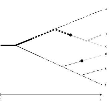
Figure 6: The branching process with mutation and binary splitting. Bullets mark death events; line segments that are alive are shown in black, virtual ones in grey, types are indicated by various line styles. The (randomly chosen) representative line is marked fat; its initial segment shown here is the first child of the second child of the first child of the root, i.e., the individual $x=(0,1,0)$. Since it has experienced three splitting events, it is a third generation individual; but it is virtual, as in fact already its mother $(0,1)$ died. The ‘black’ tree is a realization of the branching process. The individuals alive at time $t$ constitute the population $X(t)$ (a mixture of various generations); here, $X(t)=\{(0,0),(1,1,0),(1,1,1)\}$; the other individuals at time $t$ are virtual.

For each line $\omega$, we consider now the following families of random variables: $\{M^{\omega}(t)\}_{t\geq 0}$, the type process, which associates with $t$ the type of $\omega$ at time $t$; $\{\beta^{\omega}(t)\}_{t\geq 0}$, the number of birth events along $\omega$ before $t$; and $T^{\omega}$, the time line $\omega$ dies (if $\omega$ survives forever, this time is infinite). Both the birth and the death process depend on the type process, but not vice versa. The crucial information on $\{M^{\omega}(t)\}_{t\geq 0}$ is contained in its empirical measure

$$L^{\omega}(t):=\frac{1}{t}\int_{0}^{t}\delta_{M^{\omega}(\tau)}\,d\tau\,,$$ (21)

cf. (9). For an individual $x$ at time $t$, the empirical measure only depends on the initial segment of $\omega$ that describes $x$. With this in mind, we will sometimes also write $L^{x}(t)$ rather than $L^{\omega}(t)$.

The above families of random variables are not independent between lines (they are dependent through common ancestry), but, by symmetry between the two offspring at every splitting event, they share the same marginal laws for all $\omega\in\Omega$. In particular, since mutation is not influenced by the reproduction events, the type process on any given line (regardless of the others) is a copy of the mutation process generated by $\boldsymbol{U}$. Let us choose one particular such line $\omega^{*}$, for example, by setting $\omega^{*}=(000\ldots)$, or by tossing a coin. The line $\omega^{*}$ may or may not survive, but it will always be present at least virtually. We will call it the representative line for reasons to become clear in a moment, and set $\beta(t):=\beta^{\omega^{*}}(t)$, $M(t):=M^{\omega^{*}}(t)$, $T(t):=T^{\omega^{*}}(t)$, and $L(t):=L^{\omega^{*}}(t)$. We will now see that, once we know the laws of these quantities, they can tell us a lot about the entire tree.

The basic observation is that, in generation $n$, there are $2^{n}$ possible (real or virtual) individuals, all with the same marginal laws for the random variables just discussed. This allows us to express the expected population size of a population started by a single $i$ individual at time $0$ as follows:

$$\begin{split}\mathbb{E}^{i}\big{(}\|Z(t)\|_{1}\big{)}&=\mathbb{E}^{i}\big{(}\lvert X(t)\rvert\big{)}=\sum_{n\geq 0}2^{n}\,\mathbb{E}^{i}(\mathbb{I}\{\beta(t)=n,T>t\})\\ &=\mathbb{E}^{i}\big{(}2^{\beta(t)}\mathbb{I}\{T>t\}\big{)}\,.\end{split}$$ (22)

Now, conditionally on $L(t)$, the random variables $\{T>t\}$ and $\beta(t)$ are independent, having probability $\exp(-t\langle L(t),D\rangle)$ resp. the Poisson distribution $\text{\rm Poi}_{t\langle L(t),B\rangle}$ with parameter $t\langle L(t),B\rangle$. Therefore,

$$\begin{split}\mathbb{E}(2^{\beta(t)}\mid L(t))&=\exp(t\langle L(t),B\rangle),\text{ and }\\ \mathbb{E}(\mathbb{I}\{T>t\}\mid L(t))&=\exp(-t\langle L(t),D\rangle)\end{split}$$

(both independently of the type of the root), where the former relies on the fact that, for a random variable $Y$ with distribution $\text{\rm Poi}_{\lambda}$, one has $\mathbb{E}(2^{Y})={\rm e}^{\lambda}$. Therefore, (22) turns into

$$\begin{split}\mathbb{E}^{i}\big{(}\|Z(t)\|_{1}\big{)}&=\mathbb{E}^{i}\Big{(}\mathbb{E}\big{(}2^{\beta(t)}\mathbb{I}\{T>t\}\mid L(t)\big{)}\Big{)}\\ &=\mathbb{E}^{i}\Big{(}\mathbb{E}\big{(}2^{\beta(t)}\mid L(t)\big{)}\,\mathbb{E}\big{(}\mathbb{I}\{T>t\}\mid L(t)\big{)}\Big{)}\\ &=\mathbb{E}^{i}({\rm e}^{t\langle L(t),B\rangle}{\rm e}^{-t\langle L(t),D\rangle})=\mathbb{E}^{i}({\rm e}^{t\langle L(t),R\rangle}).\end{split}$$ (23)

Note that the remaining expectation (and the outer one where expectations are nested) is with respect to $L(t)$. We also remark that the underlying tree construction lurks behind the above derivation, but in the simple case at hand it need not be made more explicit.

4.2 General splitting rules

We have, so far, restricted ourselves to the decoupled model with parallel mutation, reproduction and death. The crucial simplifiying feature here is the fact that, forward in time on every line, we have a copy of the mutation process generated by $\boldsymbol{U}$. Therefore, we could consider any line as representative.

Outside the parallel model, the decomposition $\boldsymbol{A}=\boldsymbol{U}+\boldsymbol{R}$ is formal to start with, and the generator $\boldsymbol{U}$ has no immediate interpretation. But with the help of a more advanced tree construction, one can again obtain a representative line with its type process $M(t)$ generated by $\boldsymbol{U}$. We will only give a rough sketch here; for the full picture we refer the reader to [15].

The construction relies on a so-called size-biased tree with random spine (or trunk). The general concept was introduced in [21, 30] and [28]; the particular (continuous-time) version required here can be found in [15, Remark 4.2]. Informally, one constructs a modified tree with a randomly selected, distinguished line (called the trunk or spine), along which time runs at a different rate and offspring are weighted according to their size; in particular, there is always at least one offspring along the trunk so that the trunk survives forever. The children off the trunk get ordinary (unbiased) descendant trees; see Fig. 7.

\psfrag{tau}{$\underbrace{\qquad\qquad\;}_{\tau_{j}}$}\psfrag{pj}{$\Biggr{\}}N_{j}\sim{\boldsymbol{p}}_{j}$}\psfrag{Ni}{$\Biggr{\}}\widetilde{N}_{i}\sim\widetilde{{\boldsymbol{p}}}_{i}$}\psfrag{taui}{$\underbrace{\qquad\qquad\quad\qquad\;\;}_{\widetilde{\tau}_{i}}$}\psfrag{j}{$j$}\psfrag{i}{$i$}\includegraphics{sizebias.eps}

Figure 7: A realization of a size-biased tree with its trunk (the fat line). An individual of type $j$, off the trunk, has offspring $N_{j}$ with distribution $\boldsymbol{p}_{j}$ after an exponential waiting time $\tau_{j}$ with mean $1/A_{j}$; an individual of type $i$ along the trunk bears offspring $\widetilde{N}_{i}$ with biased distribution $\tilde{\boldsymbol{p}}_{i}$ after an exponential waiting time $\tilde{\tau}_{i}$ with mean $1/A_{i}\mathbb{E}(\|N_{i}\|_{1})$.

More precisely, for each type $i\in S$, we introduce the size-biased offspring distribution

$$\tilde{\boldsymbol{p}}_{i}(\kappa)=\frac{\|\kappa\|_{1}\boldsymbol{p}_{i}(\kappa)}{\mathbb{E}(\|N_{i}\|_{1})},\quad\kappa\in\mathbb{Z}_{\geq 0}^{S}.$$

Starting at the root, an individual of type $i$ on the trunk waits for an exponential time with parameter $A_{i}\mathbb{E}(\|N_{i}\|_{1})$ and then produces offspring $\tilde{N}_{i}$ according to $\tilde{\boldsymbol{p}}_{i}$; one of these offspring is chosen randomly (with equal weight) as the successor on the trunk. It is easily verified that the type process on the trunk is a Markov chain generated by $\boldsymbol{U}$. The trunk takes the role of the representative line, and the considerations of the previous Subsection carry over. We do not spell this out here explicitly; for the complete picture and many details, in particular on how the trunk may be used to extract further information about the tree, see [15]. To avoid misunderstandings, we would like to emphasize that the size-biased tree as applied to the parallel model does not reduce to the simple special construction of the previous Subsection. In particular, unlike the representative line of this construction, the trunk of the size-biased tree is certain to survive forever. However, both constructions share the essential property that the mutation process along the trunk or representative line, respectively, is generated by $\boldsymbol{U}$, and the fact that many properties of the entire tree may be extracted from this distinguished line.

5 Variational characterization of the asymptotic growth rate

We are now in a position to derive the variational characterization (11) of the asymptotic growth rate $\lambda$. The idea is to observe both the mutation process and the reproduction rate along the representative line of the tree. The appropriate tool for analyzing the tradeoff between these processes is the large deviation principle for the mutation process.

5.1 Using the large deviation principle

Let us, for the moment, restrict ourselves to the parallel model; we will see later that our results hold automatically for general splitting rules. For the parallel model, we can combine (6) and (23) to obtain

$$\lambda=\lim_{t\to\infty}\frac{1}{t}\log\mathbb{E}^{i}({\rm e}^{t\langle L(t),R\rangle})=\lim_{t\to\infty}\frac{1}{t}\log\mathbb{E}^{i}\Big{(}\exp\big{[}\textstyle\int_{0}^{t}R_{M(\tau)}\,d\tau\big{]}\Big{)}\,,$$ (24)

that is, the growth rate can be determined by observing the types and the associated reproduction rates along the representative line. The competition between reproduction and mutation will lead to a variational formula for $\lambda$, which can immediately be derived from the variational formulas of large deviation theory. The basic fact is the following large deviation principle for $L(t)$, see [20, Ch. III.1 and IV.4] or [7, Ch. 1.2 and 3.1]).

Proposition 1

The empirical measure $L(t)$ of a continuous-time Markov chain on a finite state space $S$ with irreducible generator $\boldsymbol{U}$ satisfies the large deviation principle (LDP) with rate function

$$I_{\boldsymbol{U}}(\nu):=\sup_{v>0}\Big{[}-\Big{\langle}\nu,\frac{\boldsymbol{U}v}{v}\Big{\rangle}\Big{]},\qquad\nu\in\mathsf{P}(S),$$ (25)

where the supremum is taken over all $v\in\mathbb{R}_{>0}^{S}$, and the fraction is to be understood component-wise, i.e., $\boldsymbol{U}v/v$ is the vector with components $(\boldsymbol{U}v)_{i}/v_{i}$. More explicitly, the LDP means that

$$\limsup_{t\to\infty}\frac{1}{t}\log\mathbb{P}\big{(}L(t)\in C\big{)}\leq-\inf_{\nu\in C}I_{\boldsymbol{U}}(\nu)\$$

for any closed set $C\subset\mathsf{P}(S)$, and

$$\liminf_{t\to\infty}\frac{1}{t}\log\mathbb{P}\big{(}L(t)\in O\big{)}\geq-\inf_{\nu\in O}I_{\boldsymbol{U}}(\nu)\$$

for any open set $O\subset\mathsf{P}(S)$. Furthermore, $I_{\boldsymbol{U}}$ is continuous, strictly convex and nonnegative, and $I_{\boldsymbol{U}}(\nu)=0$ precisely for $\nu=\rho$, the stationary distribution of $\boldsymbol{U}$.

For an informal statement of the LDP recall (10). (Although we have stated the LDP here only for the special case we need, it is indeed quite a general principle that applies to many common types of random variables. We refer the interested reader to the monographs [7] or [20].)

Returning to (24), we now see that, on the right-hand side, the exponential factor ${\rm e}^{t\langle L(t),R\rangle}$ is integrated over a probability measure that behaves essentially like ${\rm e}^{-tI_{\boldsymbol{U}}}$. It may thus be evaluated by Varadhan’s lemma on the asymptotics of exponential integrals, which is a far-reaching generalization of Laplace’s method; see [20, Thm. III.13] or [7, Thm. 4.3.1]. Specifically, we obtain the key formula

$$\lambda=\lim_{t\to\infty}\frac{1}{t}\log\int_{\mathsf{P}(S)}{\rm e}^{t\langle\nu,R\rangle}\,\mathbb{P}^{i}(L(t)\in{\,\rm d}\nu)=\max_{\nu\in\mathsf{P}(S)}\big{[}\langle\nu,R\rangle-I_{\boldsymbol{U}}(\nu)\big{]},$$ (26)

which may be understood as a ‘largest exponent wins’ principle. Let us continue with a series of comments.

5.1.1 Relation to the retrospective process. The maximum principle (26), though derived by considering the branching process forward in time, is directly connected to the retrospective process of (8). In analogy with (25), the rate function for the empirical measure of the retrospective process (generated by $\boldsymbol{G}$ of (8)) reads $I_{\boldsymbol{G}}(\nu)=\sup_{w>0}[-\langle\nu,(\boldsymbol{G}w)/w\rangle]$. This, however, is closely related to $I_{\boldsymbol{U}}(\nu)$. Indeed, setting $v=(v_{i})_{i\in S}$ with $v_{i}=h_{i}w_{i}$ we can write $\langle\nu,(\boldsymbol{G}w)/w\rangle=\sum_{i,j\in S}\nu_{i}(A_{ij}-\lambda\delta_{ij})h_{j}w_{j}/h_{i}w_{i}=\sum_{i,j\in S}\nu_{i}(A_{ij}-\lambda\delta_{ij})v_{j}/v_{i}=\langle\nu,R\rangle-\lambda+\langle\nu,(\boldsymbol{U}v)/v\rangle$, whence

$$\begin{split}I_{\boldsymbol{G}}(\nu)&=\sup_{w>0}[-\langle\nu,(\boldsymbol{G}w)/w\rangle]=\lambda-\langle\nu,R\rangle+\sup_{v>0}[-\langle\nu,(\boldsymbol{U}v)/v\rangle]\\ &=\lambda-\langle\nu,R\rangle+I_{\boldsymbol{U}}(\nu)\,.\end{split}$$ (27)

Again, $I_{\boldsymbol{G}}(\nu)$ is nonnegative, strictly convex, and vanishes if and only if $\nu=\alpha$, the stationary distribution of $\boldsymbol{G}$. It follows that the ancestral distribution $\alpha$ is the unique maximizer in (26). We may thus summarize our findings in the following theorem (recall (6) for the first identity).

Theorem 5.1

The forward-time stationary distribution $\pi$, the reproduction rate $R$, the asymptotic growth rate $\lambda$, the mutation process $\boldsymbol{U}$ and the ancestral distribution $\alpha$ are linked via the equation

$$\langle\pi,R\rangle=\lambda=\max_{\nu\in\mathsf{P}(S)}\big{[}\langle\nu,R\rangle-I_{\boldsymbol{U}}(\nu)\big{]}=\langle\alpha,R\rangle-I_{\boldsymbol{U}}(\alpha)\,.$$ (28)

5.1.2 The mutation rate function at the ancestral distribution. Thm. 5.1 yields the additional relation

$$I_{\boldsymbol{U}}(\alpha)=\langle\alpha,R\rangle-\lambda=\langle\pi,Rh-\boldsymbol{A}h\rangle=\langle\pi,-\boldsymbol{U}h\rangle=\sum_{\begin{subarray}{c}i,j\in S:\\ i\neq j\end{subarray}}\pi_{i}U_{ij}(h_{i}-h_{j}),$$

i.e., the value of the mutational rate function at the optimum equals the long-term loss of offspring due to mutation, wherefore it was previously termed mutational loss function; see [18, Sec. 5 and Appendix A] for the biological implications.

5.1.3 Balance of mutation and reproduction. On every line $\omega$, the mutation process runs randomly through a sequence of histories, and hence determines an evolution of empirical measures $L^{\omega}(t)\in\mathsf{P}(S)$. As $t\to\infty$, the empirical measures $\nu=L^{\omega}(t)$ that differ from the stationary distribution $\rho$ of $\boldsymbol{U}$ become exponentially less probable at asymptotic rate $I_{\boldsymbol{U}}(\nu)$. In particular, $\rho$ is the (almost-sure) long-term time average on the line $\omega$ in the forward direction of time. In spite of this, the long-term population average $\pi$ of (5) differs from $\rho$, in general. This is because mutation is counterbalanced by reproduction, at rate $R_{M^{\omega}(t)}$ at instant $t$, and at mean rate $\langle L^{\omega}(t),R\rangle$ for the entire line segment up to time $t$. We note that in realistic biological models the largest reproduction rates typically belong to types that are improbable under the stationary mutation distribution $\rho$ (‘good’ types are rare under mutation alone, otherwise it would not require selection to establish them!). Hence, empirical measures with a large mean reproduction rate tend to differ markedly from $\rho$. The resulting tradeoff between the mean reproduction rate of a line and its asymptotic rate of decay is won by those lines $\omega$ for which $L^{\omega}(t)=\nu$ maximizes the difference, $\langle\nu,R\rangle-I_{\boldsymbol{U}}(\nu)$. According to Thm. 5.1, these are precisely the lines having the ancestral distribution $\alpha$ as their time average. It is therefore this $\alpha$ that is successful in the long run and that we see when looking back into the past.

5.1.4 Extension to general splitting rules. In our proof of Thm. 5.1 above, we used a probabilistic argument that relied on the parallel model and the associated tree construction. So it might seem that this theorem is limited to this particular model. Note, however, that all quantities appearing in Thm. 5.1 are solely determined by the first-moment generator $\boldsymbol{A}$ of the process, so that it is a property of $\boldsymbol{A}$ rather than the underlying process. For an arbitrary Markov branching process, we can use the formal decomposition $\boldsymbol{A}=\boldsymbol{U}+\boldsymbol{R}$ of its first-moment generator to build a parallel model with the same $\boldsymbol{A}$. Since the theorem holds for the latter process, it also holds for the former; this is some kind of “invariance principle”. All that is lost is the probabilistic interpretation given in the previous comment; such an interpretation may be regained with the help of the size-biased tree construction of Subsec. 4.2, but is then more involved.

5.2 Reversible mutation rates, and symmetrization

We will now discuss the important special case that $\boldsymbol{U}$ is reversible, in that $\rho_{i}U_{ij}=\rho_{j}U_{ji}$ for all $i,j\in S$. This is assumed in most models of nucleotide evolution, see, e.g., [12, Ch. 13]. The interest in this case comes from the following facts.

5.2.1 Explicit form of the rate function. For reversible $\boldsymbol{U}$, the maximization in (25) can be carried out explicitly, so that the rate function takes the closed form [20, p. 50, Ex. IV.24]

$$I_{\boldsymbol{U}}(\nu)=-\Big{\langle}\text{\small$\sqrt{\frac{\nu}{\rho}},\,\boldsymbol{U}\sqrt{\frac{\nu}{\rho}}$ }\Big{\rangle}_{\!\rho}\,;$$ (29)

here both the square root and the fraction are to be read componentwise, and $\langle u,v\rangle_{\rho}$ denotes the Dirichlet form $\sum_{i}u_{i}v_{i}\rho_{i}$ for vectors $u,v$, and $\rho$. (It is an interesting fact that no such simplification exists for reversible Markov chains in discrete time.) Noting that $\rho_{i}>0$ for all $i\in S$ by irreducibility, using the reversibility in the form $\sqrt{\rho_{i}/\rho_{j}}\,U_{ij}=\sqrt{U_{ij}U_{ji}}$, and recalling that $U_{ii}=-\sum_{j:j\neq i}U_{ij}$, one readily finds that Eq. (29) is equivalent to

$$I_{\boldsymbol{U}}(\nu)=\frac{1}{2}\sum_{i,j\in S:\,i\neq j}\big{(}\sqrt{\nu_{i}U_{ij}}-\sqrt{\nu_{j}U_{ji}}\big{)}^{2}.$$ (30)

5.2.2 Estimation of the reproduction rate from the ancestral distribution. The reversibility of $\boldsymbol{U}$ immediately implies that the vector $\rho h:=(\rho_{i}h_{i})_{i\in S}$ is a left eigenvector of $\boldsymbol{A}=\boldsymbol{U}+\boldsymbol{R}$ for the principal eigenvalue $\lambda$, cf. [3]. Hence $\pi=\rho h$ up to a normalization factor, and therefore $\alpha=\rho h^{2}$, or $h=\sqrt{\alpha/\rho}$, again up to a normalization factor. (As before, the square root and the fraction are to be read componentwise.) This in turn means that $\alpha$, together with $\rho$, determines the reproduction rate $R$ up to an additive constant. Indeed, suppose that $R$ and $R^{\prime}$ are two reproduction rates (for the same mutation matrix $\boldsymbol{U}$) having the same ancestral distribution $\alpha=\alpha^{\prime}$. Then $h=h^{\prime}$, whence $(R-R^{\prime})h=(\lambda-\lambda^{\prime})h$. As $h$ is strictly positive, it follows that all components of $R-R^{\prime}$ agree.

5.2.3 Symmetrized mutation rates. For reversible $\boldsymbol{U}$, one can introduce the matrix $\widetilde{\boldsymbol{A}}:=(\tilde{A}_{ij})_{i,j\in S}$ by $\tilde{A}_{ij}=\sqrt{\rho_{i}}A_{ij}/\sqrt{\rho_{j}}$, which is symmetric and has the same spectrum as $\boldsymbol{A}=\boldsymbol{U}+\boldsymbol{R}$. The maximum principle of Thm. 5.1 can therefore also be derived from the Rayleigh-Ritz (or Courant-Fisher) variational principle for the leading eigenvalue of $\widetilde{\boldsymbol{A}}$; see [3, Sec. 2]. We emphasize, however, that the large deviation approach to (26) is not tied to reversible matrices and, as we have shown above, admits a natural interpretation in terms of the underlying family tree. Nevertheless, we will take advantage of the symmetrization $\widetilde{\boldsymbol{A}}$ in Sect. 7 below. In particular, we will use the (unique) decomposition $\widetilde{\boldsymbol{A}}=\boldsymbol{F}+\boldsymbol{E}$ into a symmetric Markov generator $\boldsymbol{F}=(F_{ij})_{i,j\in S}$, defined through

$$F_{ij}=\begin{cases}\sqrt{U_{ij}U_{ji}}=F_{ji}&\text{for }i\neq j,\\ -\sum_{k\in S\setminus\{i\}}\sqrt{U_{ik}U_{ki}}&\text{for }i=j\,,\end{cases}$$ (31)

and a diagonal matrix $\boldsymbol{E}:=\text{diag}(E_{i}\mid i\in S)$ with elements

$$E_{i}:=\sum_{j\in S}\tilde{A}_{ij}=R_{i}+U_{ii}-F_{ii}=R_{i}+\sum_{j\in S}\sqrt{U_{ij}U_{ji}}\,.$$ (32)

6 Unfolding the variational principle

As we have seen, the maximum principle of Thm. 5.1 provides some general insight into the competition, and resulting tradeoff, between mutation and reproduction. In general, however, it can not be solved explicitly. This is because both the maximization over the space $\mathsf{P}(S)$, and the eigenvalue equations determining $\pi$, $h$ and thus $\alpha$, are $|S|$-dimensional, and $S$ is typically large. It is thus natural to ask whether one can obtain a low-dimensional variational principle in a specific setting. In the rest of this paper we will therefore confine ourselves to genetic models of sequence type where each type is specified by a sequence of letters from a finite alphabet. The variational problem can then be split into two simpler ones, a constrained variational principle with fixed mean letter composition, and a maximization over all possible constraints. In some cases, each of these two subproblems may be treated explicitly or, at least, approximately.

6.1 Lumping of sequence types, or: Choice of a type space

As previewed in Subsection 3.2, we will now assume that the type of an individual is characterized by a sequence of letters from some finite alphabet $\varSigma$, which leads to the type space $\varSigma^{N}$. If we assume that the mutation and reproduction rates are invariant under permutations of sequence sites, as we will do in what follows, this sequence space can be lumped into the smaller space

$$S=\Big{\{}i\in\mathbb{Z}^{d}\mid i_{\ell}\geq 0\>\text{for}\>\ell\in\varSigma,\;\sum_{\ell\in\varSigma}i_{\ell}=N\Big{\}}\,,$$ (33)

recall Fig. 5. For example, this is possible for sequence space models with parallel mutation and reproduction, in which

1. all sites mutate independently and according to the same (Markov) process (a natural first assumption made in many models of sequence evolution) and

2. the fitness function is invariant under permutation of sites (a less natural, but still common assumption that applies, for example, if fitness only depends on the sequence through the number of mutated positions (i.e., the Hamming distance) relative to a reference sequence, often termed the ‘wildtype’);

see, e.g., [18, 14] or [16] for previous work on this case. (As an alternative to the choice (33), one can use the constraint $\sum_{\ell\in\varSigma}i_{\ell}=N$ to remove an element $a\in\varSigma$ by setting $\varSigma^{*}=\varSigma\setminus\{a\}$ and work instead with

$$S^{*}=\Big{\{}i\in\mathbb{Z}^{d}\mid i_{\ell}\geq 0\>\text{for}\>\ell\in\varSigma^{*},\;\sum_{\ell\in\varSigma^{*}}i_{\ell}\leq N\Big{\}}\,,$$ (34)

where now $d=\lvert\varSigma^{*}\rvert=\lvert\varSigma\rvert-1$.)

Specifically, if the reproduction and mutation rates on $\varSigma^{N}$ are given by $\mathcal{R}_{\sigma}$ and $\mathcal{U}_{\sigma\tau}$ ($\sigma,\tau\in\varSigma^{N}$), then, by permutation invariance, there is a vector $R=(R_{i})_{i\in S}$ and a Markov generator $\boldsymbol{U}=(U_{ij})_{i,j\in S}$ so that $\mathcal{R}_{\sigma}=R_{H(\sigma)}$ and $\sum_{\tau:H(\tau)=j}\mathcal{U}_{\sigma\tau}=U_{H(\sigma),j}$ for all $\sigma\in\varSigma^{N}$; here $H$ is as in (12). $R$ and $\boldsymbol{U}$ then define a Markovian branching process with type space $S$.

In fact, assumption (L1) even implies that the mutation rates $U_{ij}$ of the lumped model are linear in $i\in S$ (or affine in $i\in S^{*}$). This is seen as follows: If $w_{\ell m}$ is the mutation rate (at every site) from letter $\ell$ to letter $m$, then the corresponding transition in the lumped model (based on $\varSigma$) is $i\to i-e_{\ell}+e_{m}$ (where $e_{j}$ is the the unit vector in $\boldsymbol{R}^{d}$ having a 1 at coordinate $j$), and occur at rates $i_{\ell}w_{\ell m}$, due to independence of the sites. If, instead, one removes one dimension by setting $i_{a}=N-\sum_{\ell\in\varSigma^{*}}i_{\ell}$ and then works with $\varSigma^{*}$, one obtains the additional transitions $i\to i-e_{\ell}$ at rate $w_{\ell a}i_{\ell}$, and $i\to i+e_{m}$ at the (affine) rate $w_{am}(N-\sum_{\ell\in\varSigma^{*}}i_{\ell})$.

Assumption (L2) is less specific than (L1); the fitness function in the lumped model will, in general, be nonlinear due to interactions between sites. It will, however, turn linear (or affine) if fitness contributions are additive across sites, as is usually assumed in, e.g., models of codon bias (where $\varSigma$ is the set of possible codons). Additivity reflects independent fitness contributions of the sites and means that, for $i\in S$, one has $R_{i}=\sum_{\ell\in\varSigma}r_{\ell}\,i_{\ell}$ (based on $\varSigma$), or $R_{i}=r_{a}N+\sum_{\ell\in\varSigma^{*}}^{d}(r_{\ell}-r_{a})i_{\ell}$ (if $\varSigma^{*}$ is used), where $r_{\ell}\in\mathbb{R}$ for $\ell\in\varSigma$. We will examine such linear models in Subsec. 6.3.

6.2 Fixing the empirical mean

The only property of the special choices (33) or (34) of the type space $S$ we need at the moment is that $S\subset\mathbb{R}^{d}$. This provides $S$ with the structure of an abelian group (elements of $S$ can be added and subtracted), and allows us to classify the possible empirical distributions $\nu\in\mathsf{P}(S)$ according to the value of their mean $\langle\nu,\mathrm{id}\rangle\in\mathbb{R}^{d}$. In particular, for the random measure $L^{\omega}(t)$ of (21), $\langle L^{\omega}(t),\mathrm{id}\rangle$ is a random vector in $\mathbb{R}^{d}$, namely the empirical mean, or empirical mean letter composition along the line $\omega$ up to time $t$. If $S$ is obtained through lumping a sequence space $\varSigma^{N}$ as in Fig. 5, the $\ell$’th coordinate of $L^{\omega}(t)$ indicates the total fraction of time up to $t$ for which some site in the sequence characterizing an individual on the line $\omega$ shows letter $\ell\in\varSigma$. Note that this involves a twofold averaging, namely an average over time and a (non-normalized) average over sequence sites.

As indicated in (14) and (15), we will now foliate the variational formula (26) by prescribing the mean of the underlying type distribution. That is, we write

$$\lambda=\max_{z\in\text{conv}\>S}\Lambda(z),$$ (35)

where

$$\Lambda(z):=\max_{\begin{subarray}{c}\nu\end{subarray}\in\mathsf{P}(S):\\ \langle\nu,\mathrm{id}\rangle=z}\;[\langle\nu,R\rangle-I_{\boldsymbol{U}}(\nu)]$$ (36)

is the constrained mean fitness of $z\in\text{conv}\>S$. As before, the maxima are attained by continuity, and the maximizer in (36) is unique by the strict convexity of $I_{\boldsymbol{U}}$. The function $\Lambda$ is strictly concave; this follows again from the strict convexity of $I_{\boldsymbol{U}}$, together with the linearity of $\langle\,\cdot\,,R\rangle$ and $\langle\,\cdot\,,\mathrm{id}\rangle$. In particular, $\Lambda$ is continuous on

$$\text{rint\,conv}\>S=\big{\{}\langle\nu,\mathrm{id}\rangle\mid\nu\in\mathsf{P}(S),\,\nu_{i}>0\text{ for all }i\in S\big{\}}\,,$$

the relative interior of $\text{conv}\;S$ [32, p. 82]. In general, the relative interior $\text{rint}\>\mathsf{D}$ of a set $\mathsf{D}\subset\mathbb{R}^{d}$ is defined as the interior of $\mathsf{D}$ relative to the smallest affine subspace containing $\mathsf{D}$. Moreover, since $\alpha$ is the unique maximizer in (28), there exists a unique $\hat{z}\in\text{conv\,}S$ that maximizes $\Lambda$, namely

$$\hat{z}=\langle\alpha,\mathrm{id}\rangle,$$ (37)

i.e., the unique maximizer $\hat{z}$ in (35) is the ancestral type average.

If $\boldsymbol{U}$ is reversible, we may restrict the maximization in (35) to those $z$ that are strict convex combinations of the elements of $S$. This is obvious from the explicit form of $I_{\boldsymbol{U}}$ in (30): If at least one component of $\nu$ vanishes, one has $(\partial/\partial\nu_{i})I_{\boldsymbol{U}}(\nu)=+\infty$ for some $i$. Therefore, the maximum will be located in $\text{rint\,conv}\>S$, so that Eq. (35) can be replaced by

$$\lambda=\max_{z\in\text{rint\,conv}\,S}\Lambda(z).$$ (38)

If the function $\Lambda(z)$ were known explicitly, the variational problem of Thm. 5.1 would boil down to a maximization over a subset of $\mathbb{R}^{d}$; for small $d$ one could aim at explicit solutions. Such low-dimensional variational principles for $\lambda$ were recently derived for several examples, by methods from linear algebra and asymptotic analysis [3, 13, 14, 18]. However, a plausible understanding for the resulting function to be maximized has been lacking so far. The next Proposition reveals the probabilistic meaning of $\Lambda(z)$: It is nothing but the asymptotic growth rate of the lines having empirical type average (close to) $z$. Together with (37), this shows that the growth rate of the total population coincides with the growth rate $\Lambda(\hat{z})$ of the subpopulation consisting of all individuals with empirical type average close to the ancestral one.

Proposition 2

For all $z\in\text{rint\,conv}\,S$, the solution of the constrained variational problem (36) satisfies

$$\Lambda(z)=\lim_{\varepsilon\to 0}\lim_{t\to\infty}\frac{1}{t}\log\mathbb{E}^{i}\Big{(}\sum_{x\in X(t)}\mathbb{I}\big{\{}\|\langle L^{x}(t),\mathrm{id}\rangle-z\|_{1}\leq\varepsilon\big{\}}\Big{)}.$$

Proof

Consider first the parallel model. By the reasoning leading to (23), the growth rate of the subpopulation consisting of all individuals with empirical mean close to $z$, up to some maximal deviation $\varepsilon>0$, is equal to

$$\begin{split}\@ADDCLASS{ltx_eqn_lefteqn}$\displaystyle\lim_{t\to\infty}\frac{1}{t}\log\mathbb{E}^{i}\Big{(}\sum_{x\in X(t)}\mathbb{I}\big{\{}\|\langle L^{x}(t),\mathrm{id}\rangle-z\|_{1}\leq\varepsilon\big{\}}\Big{)}$\mbox{}\hfil\\ &=\lim_{t\to\infty}\frac{1}{t}\log\sum_{n\geq 0}2^{n}\;\mathbb{E}^{i}\Big{(}\mathbb{I}\big{\{}\beta(t)=n,\;T>t,\;\|\langle L(t),\mathrm{id}\rangle-z\|_{1}\leq\varepsilon\big{\}}\Big{)}\\ &=\lim_{t\to\infty}\frac{1}{t}\log\mathbb{E}^{i}\Big{(}{\rm e}^{t\langle L(t),R\rangle}\,\mathbb{I}\big{\{}\|\langle L(t),\mathrm{id}\rangle-z\|_{1}\leq\varepsilon\big{\}}\Big{)}\\[2.15277pt] &=\lim_{t\to\infty}\frac{1}{t}\log\mathbb{E}^{i}\Big{(}\exp\big{[}\,t\,\big{(}\langle L(t),R\rangle-\infty\cdot\mathbb{I}\{\|\langle L(t),\mathrm{id}\rangle-z\|_{1}>\varepsilon\}\big{)}\big{]}\Big{)}\\[2.15277pt] &=\max_{\nu\in\mathsf{P}(S):\,\|\langle\nu,\mathrm{id}\rangle-z\|_{1}\leq\varepsilon}\big{[}\langle\nu,R\rangle-I_{\boldsymbol{U}}(\nu)\big{]}=\max_{y\in\text{conv}\,S:\,\|y-z\|_{1}\leq\varepsilon}\Lambda(y).\end{split}$$ (39)

Here we have used the conventions $\infty\cdot 1=\infty$ and $\infty\cdot 0=0$ in the third step, and Varadhan’s lemma in the fourth, in analogy with (26); the maximum over $\nu$ is attained since the condition $\|\langle\nu,\mathrm{id}\rangle-z\|_{1}\leq\varepsilon$ defines a compact subset of $\mathsf{P}(S)$. As $\Lambda$ is continuous on $\text{rint\,conv}\,S$, the last expression converges to $\Lambda(z)$ as $\varepsilon\to 0$, as asserted.

For a general splitting rule, the argument is the same except that the particular tree construction of Subsec. 4.1 has to be replaced by the size-biased tree described in Subsec. 4.2. In fact, one simply has to omit the second line of (39) above and instead invoke Eq. (4.4) of [15] which shows that the first line of (39) coincides with the third; the random measure $L(t)$ in the third line is then again the empirical measure of a Markov chain with generator $\boldsymbol{U}$, namely the mutation process along the spine of the size-biased tree.

Like the unconstrained variational problem (26) leading to $\lambda$, the constrained problem (36) defining $\Lambda$ provides insight into the mutation-reproduction process, but does not, in general, lead to an explicit solution if $S$ is large. ¿From the point of view of explicit calculations, it rather expresses one difficult problem (the leading eigenvalue of a large matrix) in terms of another difficult problem (the maximization over a large space). But if $\boldsymbol{U}$ is reversible, there are two cases in which (36) may be solved explicitly or, at least, asymptotically. These are the cases when fitness and mutation are linear (already hinted at in Sec. 6.1), or when they allow a continuous approximation in the limit as the number $N$ of sequence sites grows large. These will be discussed in the next Subsection and in Section 7.

6.3 Exact results for linear reversible models

In this Subsection we have a closer look at the sequence space models of Sec. 6.1 that describe the independent evolution of $N$ sites with a finite alphabet $\varSigma$ and lead, after lumping, to models with state space $S$ as in (33), with linear fitness and mutation, and mutational transitions $i\to i+k$ restricted to those with $k\in\mathfrak{S}:=\{e_{m}-e_{\ell}\mid m,\ell\in\varSigma,\,m\neq\ell\}$. In line with standard assumptions on sequence evolution (see, e.g., [12, Ch. 14]), we posit that the mutation process acting at the sites is reversible, that is, the mutation rates $(w_{\ell m})_{\ell,m\in\varSigma}$ define an irreducible and reversible Markov generator with a reversible distribution $\gamma$ on $\varSigma$. After lumping, the associated mutation process on $S$ then has rates $U_{ij}=U_{j-i}(i)$ , $i,j\in S$, given by

$$U_{k}(z)=\begin{cases}w_{\ell m}z_{\ell}&\text{if }k=e_{m}-e_{\ell}\in\mathfrak{S},\\ -\sum_{\ell\neq m}w_{\ell m}z_{\ell}&\text{for }k=0,\\ 0&\text{otherwise}\end{cases}$$

for $z\in\mathbb{R}^{d}$, $d=|\varSigma|$. The reversibility of $(w_{\ell m})_{\ell,m\in\varSigma}$ readily implies that the mutation generator $\boldsymbol{U}=(U_{ij})_{i,j\in S}$ is also reversible; its reversible distribution is $\rho:=\text{\rm Mult}_{N,\gamma}$ , the multinomial distribution for $N$ samples from the distribution $\gamma$ on $\varSigma$. As motivated in Sec. 6.1, we will also assume here that the reproduction rates are linear, in that $R_{i}=R(i)$ for all $i\in S$, for a linear function $R$ of the form $R(z)=r\cdot z$, $r,z\in\mathbb{R}^{d}$. Here and below we write ‘$\cdot$’ for the scalar product of vectors in $\mathbb{R}^{d}$, in contrast to $\langle.,.\rangle$, which we have reserved for scalar products of vectors in $\mathbb{R}^{S}$. In this setting, the constrained variational problem (36) admits an explicit solution as follows. Due to (38), we may – and will – restrict ourselves to considering means in

$$\text{rint\,conv}\>S=\Big{\{}z\in\mathbb{R}^{d}\mid z_{\ell}>0\>\text{ for }\>\ell\in\varSigma,\;\sum_{\ell\in\varSigma}z_{\ell}=N\Big{\}}\,.$$

Theorem 6.1

In the situation described above, for every $z\in\text{\rm rint\,conv}\>S$ the restrained maximum of (36) is given by

$$\Lambda(z)=R(z)-\frac{1}{2}\sum_{k\in\mathfrak{S}}\Big{(}\sqrt{U_{k}(z)}-\sqrt{U_{-k}(z)}\Big{)}^{2}=\langle\nu^{(z)},R\rangle-I_{U}(\nu^{(z)}),$$ (40)

where $\nu^{(z)}=\text{\rm Mult}_{N,z/N}$ is the multinomial distribution with mean $z$.

Proof

Let $z\in\text{rint\,conv}\>S$ be given, and consider any $\nu\in\mathsf{P}(S)$ with $\langle\nu,\mathrm{id}\rangle=z$. It is then clear that $\langle\nu,R\rangle=R(z)$ by linearity. Let us rewrite Eqn. (30) in the form $I_{\boldsymbol{U}}(\nu)=\frac{1}{2}\sum_{k\in\mathfrak{S}}\|x_{k}-y_{k}\|_{2}^{2}$, where $x_{k}=(x_{k,i})_{i\in S}$ and $y_{k}=(y_{k,i})_{i\in S}$ are the vectors with components

$$x_{k,i}=\sqrt{U_{k}(i)\nu_{i}},\quad y_{k,i}=\sqrt{U_{-k}(i+k)\nu_{i+k}}\,,$$

$i\in S$, $k\in\mathfrak{S}$. In the boundary case when $i\in S$ but $i+k\notin S$, we have $U_{k}(i)=0$ by definition, and likewise $U_{-k}(i+k)=0$ when $i\notin S$ but $i+k\in S$. Hence $x_{k,i}=y_{k,i}=0$ unless $i,i+k\in S$. By linearity of the $U_{k}$, it follows that $\|x_{k}\|_{2}^{2}=U_{k}(z)$ and $\|y_{k}\|_{2}^{2}=U_{-k}(z)$ for all $k\in\mathfrak{S}$. As the distance between any two vectors is minimized when the vectors are parallel, we conclude further that

$$\|x_{k}-y_{k}\|_{2}^{2}\geq\big{(}\|x_{k}\|_{2}-\|y_{k}\|_{2}\big{)}^{2}$$

with equality if and only if there is a positive constant $C_{k}$ so that

$$U_{k}(i)\nu_{i}=C_{k}U_{-k}(i+k)\nu_{i+k}$$

whenever $i,i+k\in S$. This, however, is the case when $\nu=\nu^{(z)}$ because, for each $i\in S$, $\nu^{(z)}_{i}=e^{\beta\cdot i}\rho_{i}$ for $\beta=\log({z}/{N\gamma})$ (where the fraction and the logarithm are taken componentwise), and $\rho$ is reversible; in fact we have $C_{k}={\rm e}^{-\beta\cdot k}$. Combining the preceding observations we get the result.

If we turn from the linear model to the affine one, by removing one coordinate as indicated at the close of Sec. 6.1, Theorem 6.1 clearly remains true, with the middle expression in (40) expressed in terms of the reduced coordinates. Eq. (40) has been derived previously for certain specific choices for the mutation rates [14, 18]; remarkably, the above result provides both an extension (to arbitrary reversible models), and a simplification of the proof.

6.4 Partial convex conjugation

On our way to the second case of an explicit version of $\Lambda(z)$, we need a general intermediate step: a relation between $\Lambda(z)$ and the mean growth rate $\lambda$ for a suitably modified reproduction rate $R$. This relationship is based on partial convex conjugation, a standard procedure of convex analysis which will be spelt out here for our purposes. In Sec. 7, this will allow us to determine the asymptotic behaviour of $\Lambda(z)$ when the number $N$ of sequence sites gets large.

Let us rewrite equation (26) in the form

$$\lambda(R)=\max_{\nu\in\mathsf{P}(S)}\big{[}\langle\nu,R\rangle-I_{\boldsymbol{U}}(\nu)\big{]}$$

indicating the dependence on $R$; $\boldsymbol{U}$ will be considered as fixed. The following proposition asserts that the function $z\to-\Lambda(z)$ of constrained extrema is a partial convex conjugate of the function $R\to\lambda(R)$.

Proposition 3

Let $S\subset\mathbb{R}^{d}$, $z\in\text{\rm rint\,conv\,}S$, and $\boldsymbol{U}$ be an irreducible Markov generator on $S$ (not necessarily reversible). Then the constrained variational problem (36) has the solution

$$\begin{split}\Lambda(z)&=\inf_{\beta\in\mathbb{R}^{d}}\big{[}\lambda(R+\beta\cdot\mathrm{id})-\beta\cdot z\big{]}\\ &=\lambda(R+\beta^{z}\cdot\mathrm{id})-\beta^{z}\cdot z=\langle\alpha^{z},R\rangle-I_{\boldsymbol{U}}(\alpha^{z})\,.\end{split}$$

Here, $\beta^{z}\in\mathbb{R}^{d}$ is the negative slope vector of any tangent plane to $\Lambda$ at $z$, and $\alpha^{z}$ is the unique ancestral distribution corresponding to the reproduction rate $R+\beta^{z}\cdot\mathrm{id}$ for any such $\beta^{z}$. In particular, the function $\beta\to\lambda(R+\beta\cdot\mathrm{id})$ is differentiable on $\mathbb{R}^{d}$, and $\nabla_{\!\beta\,}\lambda(R+\beta\cdot\mathrm{id})\mid_{\,\beta=\beta^{z}}\,=\langle\alpha^{z},\mathrm{id}\rangle=z$.

Proof

For any $z\in\text{rint\,conv\,}S$ and $\beta\in\mathbb{R}^{d}$ we have, writing $\nu^{z}$ for the maximizer in (36) and using Thm. 5.1,

$$\Lambda(z)=\langle\nu^{z},R+\beta\cdot\mathrm{id}\rangle-\beta\cdot z-I_{\boldsymbol{U}}(\nu^{z})\leq\lambda(R+\beta\cdot\mathrm{id})-\beta\cdot z\,.$$

Taking the infimum over $\beta$ we arrive at the inequality

$$\Lambda(z)\leq\inf_{\beta\in\mathbb{R}^{d}}[\lambda(R+\beta\cdot\mathrm{id})-\beta\cdot z]\,.$$ (41)

To show equality we recall that $\Lambda$ is strictly concave and finite on a (relative) neigbourhood of $z$ and therefore admits a tangent plane at $z$. That is, there exists some $\beta\in\mathbb{R}^{d}$ such that

$$\Lambda(y)\leq\Lambda(z)-\beta\cdot(y-z)\quad\text{ for all }y\in\text{conv }S\,,$$

with strict inequality for $y\neq z$. Denoting by $\alpha^{\beta}$ the ancestral distribution for the reproduction rate $R+\beta\cdot\mathrm{id}$ and letting $y=\langle\alpha^{\beta},\mathrm{id}\rangle$ we find

$$\begin{split}\lambda(R+\beta\cdot\mathrm{id})-\beta\cdot z&=\langle\alpha^{\beta},R\rangle+\beta\cdot(y-z)-I_{\boldsymbol{U}}(\alpha^{\beta})\\ &\leq\,\Lambda(y)+\beta\cdot(y-z)\,\leq\,\Lambda(z)\,.\end{split}$$ (42)

Together with (41) it follows that equality holds everywhere in (42). Hence $y=z$, (41) holds with equality, and the infimum is attained for any $\beta$ determining a tangent to $\Lambda$ at $z$. In general, there may be several such tangents, e.g., if $S$ is contained in a hyperplane of $\mathbb{R}^{d}$. However, the associated ancestral distribution is uniquely determined. For, suppose there exist $\beta_{1}\neq\beta_{2}$ both determining a tangent to $\Lambda$ at $z$, and let $\alpha^{1}$ and $\alpha^{2}$ be the ancestral distributions for the reproduction rates $R+\beta_{1}\cdot\mathrm{id}$ and $R+\beta_{2}\cdot\mathrm{id}$, respectively. The preceding argument then holds for every $\beta$ in the segment $[\beta_{1},\beta_{2}]$, whence (42) holds with equality everywhere for all these $\beta$. We can thus conclude that the function $\beta\to\lambda(R+\beta\cdot\mathrm{id})$ is affine on $[\beta_{1},\beta_{2}]$. In particular, using Thm. 5.1 and the shorthand $f_{i}(\nu)=\langle\nu,R+\beta_{i}\cdot\mathrm{id}\rangle-I_{\boldsymbol{U}}(\nu)$ we find

$$\max_{\nu}\big{[}\frac{1}{2}f_{1}(\nu)+\frac{1}{2}f_{2}(\nu)\big{]}=\frac{1}{2}\max_{\nu}f_{1}(\nu)+\frac{1}{2}\max_{\nu}f_{2}(\nu).$$

Since $f_{1}$ and $f_{2}$ are strictly concave, this is only possible if they have the same maximizer. That is, $\alpha^{1}=\alpha^{2}$. Finally, using the equality in (41) and the convex duality lemma [7, Lemma 4.5.8] we find that the function $\beta\to\lambda(R+\beta\cdot\mathrm{id})$ is the convex conjugate of the strictly convex function $-\Lambda$, and thus differentiable; see [32, Thm. 26.3, p.253]. Its gradient at $\beta^{z}$ necessarily coincides with $z$.

In the case of a reversible mutation matrix $\boldsymbol{U}$, the preceding proposition can be complemented as follows. We write $T=\text{\rm span}(S-S)\subset\mathbb{R}^{d}$ for the linear space generated by the set of differences of elements of $S$.

Corollary 1

For reversible $\boldsymbol{U}$ the following additional statements hold.
(a) The function $\Lambda$ defined in (36) is differentiableon $\text{\rm rint\,conv\,}S$, and its conjugate function $\beta\to\lambda(R+\beta\cdot\mathrm{id})$ is strictly convex on $T$. Moreover, for $z\in\text{\rm rint\,conv\,}S$ and $\beta\in T$ we have $\beta=-\nabla\Lambda(z)$ if and only if $z=\nabla_{\!\beta\,}\lambda(R+\beta\cdot\mathrm{id})$.
(b) The function $\Lambda$ on $\text{\rm rint\,conv\,}S$ remains unchanged under symmetrization, i.e., by replacing $\boldsymbol{U}$ with the matrix $\boldsymbol{F}$ of (31), and $R$ with the function $E$ defined in (32).

Proof

(a) Let $z\in\text{rint\,conv\,}S$ and $\beta,\beta^{\prime}$ be two negative slope vectors of $\Lambda$ at $z$. In view of the uniqueness of $\alpha^{z}$ and the remarks in 5.2.2, the scalar product $(\beta-\beta^{\prime})\cdot i$ is then independent of $i\in S$. This means that $\beta-\beta^{\prime}$ is orthogonal to $T$, so that there is a unique negative slope vector $\beta^{z}\in T$. By concavity, the uniqueness of the tangent plane is equivalent to differentiability; cf. [32, Thm. 25.1, p. 242]. By the proof of Prop. 3, this is also equivalent to strict convexity of $\lambda(R+\beta\cdot\mathrm{id})$ on $T$. The final statement comes from the observation that both assertions are equivalent to the identity $\lambda(R+\beta\cdot\mathrm{id})-\Lambda(z)=\beta\cdot z$.

(b) For each $\beta\in\mathbb{R}^{d}$, the matrix $\boldsymbol{F}+\text{diag}(E_{i}+\beta\cdot i\mid i\in S)$ is similar to $\boldsymbol{U}+\text{diag}(R_{i}+\beta\cdot i\mid i\in S)$, so that their principal eigenvalues agree. The result thus follows from Prop. 3 by minimization over $\beta$.

7 Smooth approximations

While still adhering to a lumped sequence model, we will now turn to a situation complementary to that of Thm. 6.1: we consider nonlinear reproduction and mutation rates that allow for a continuous approximation if the number of sequence sites becomes large; this approximation is only required locally, which provides much more freedom, and, in particular, removes constraints imposed by the boundary (recall the boundary conditions $U_{k}(i)=0$ for $i\in S$, $i+k\notin S$ in Thm. 6.1). For a large family of models with reversible $\boldsymbol{U}$, an asymptotic low-dimensional maximum principle for $\lambda$ is available then [3], but no connection to the constrained mean fitness (36) has been made there, and the ensuing probabilistic interpretation was still lacking. On the basis of Prop. 3, this can now be provided.

In view of Corollary 1(b), the case of a reversible mutation matrix $\boldsymbol{U}$ can be reduced to the case of a symmetric mutation matrix $\boldsymbol{F}$. That is, instead of the first moment generator $\boldsymbol{A}=\boldsymbol{U}+\boldsymbol{R}$ we can and will consider the symmetrized version $\widetilde{\boldsymbol{A}}=\boldsymbol{E}+\boldsymbol{F}$ defined in (31) and (32). In Subsection 7.1 we will present a slight refinement of an asymptotic maximum principle derived in [3, Thm. 1]. In Subsection 7.2 we will derive an approximation of $\Lambda(z)$ in two particularly interesting situations. An application to the quasispecies model follows in Sec. 8.

7.1 Approximation of the asymptotic growth rate $\lambda$

Consider the following setup. For each $N$ let

• $S=S(N)\subset\mathbb{Z}^{d}$ be a state space as in (33) or (34).

The rescaled set $\frac{1}{N}S$ is then contained in a simplex $\mathsf{D}\subset\mathbb{R}^{d}$, viz. either $\mathsf{D}=\text{conv}\>\{e_{1},\ldots,e_{d}\}$ or $\mathsf{D}=\text{conv}\>\{0,e_{1},\ldots,e_{d}\}$, with $e_{1},\ldots,e_{d}$ the unit vectors of $\mathbb{Z}^{d}$. (In the first case, $\mathsf{D}$ is contained in a hyperplane, whence in the following we will always consider the relative interior of $\mathsf{D}$ rather than simply its interior.) In the limit as $N\to\infty$, $\frac{1}{N}S$ becomes dense in $\mathsf{D}$. For each $N$ let also

• $\boldsymbol{F}$ be a symmetric Markov generator on $S$, and $\boldsymbol{E}:=\text{diag}(E_{i}\mid i\in S)$ a diagonal matrix.

We assume that $\boldsymbol{F}$ and $\boldsymbol{E}$ admit a continuous approximation as follows: There exist real functions $e$ and $f_{k}$ on $\mathsf{D}$, and an “approximation domain” $\mathsf{A}\subset\text{rint}\,\mathsf{D}$ such that the following conditions hold.

(A1)

$e$ is $C^{2}$ on $\mathsf{A}$ and, as $N\to\infty$,

$$E_{i}=e\Big{(}{\text{\small$\frac{i}{N}$}}\Big{)}+\mathcal{O}\Big{(}\text{\small$\frac{1}{N}$}\Big{)}\quad\text{and}\quad F_{ij}=f_{j-i}\Big{(}{\text{\small$\frac{i}{N}$}}\Big{)}+\mathcal{O}\Big{(}\text{\small$\frac{1}{N}$}\Big{)}\,,$$

where the $\mathcal{O}(1/N)$ terms are uniform for all $i,j\in S$ with $i/N,j/N\in\mathsf{A}$.

(A2)

Uniformly for all $i$ with $i/N\in\mathsf{A}$,

$$\sum_{k\in S-i}f_{k}\Big{(}{\text{\small$\frac{i}{N}$}}\Big{)}\,\lvert k_{\ell}\rvert k_{m}^{2}\leq C$$

for some constant $C$ and all $1\leq\ell,m\leq d$, where $S-i:=\{j-i:j\in S\}$.

(A3)

For suitable constants $C^{\prime},C^{\prime\prime}<\infty$ we have

$$-C^{\prime}\leq E_{i}\leq\sup_{z\in\mathsf{D}}e(z)+\mathcal{O}\Big{(}\text{\small$\frac{1}{N}$}\Big{)}\quad\text{and}\quad F_{ij}\leq C^{\prime\prime}$$

for all $i,j\in S$, $i\neq j$, with a uniform error term $\mathcal{O}(1/N)$.

Theorem 7.1

Suppose the conditions (A1)–(A3) hold for a relatively open neighbourhood $\mathsf{A}$ of a global maximizer $z^{*}\in\text{rint}\,\mathsf{D}$ of $e$. Then the principal eigenvalue $\lambda$ of the matrix $\widetilde{\boldsymbol{A}}=\boldsymbol{E}+\boldsymbol{F}$ admits the approximation

$$\lambda=e(z^{*})+\mathcal{O}\Big{(}\text{\small$\frac{1}{N}$}\Big{)}.$$

The error term here only depends on the constants in (A1)–(A3) and the Hessian of $e$ at $z^{*}$ (via an upper bound on the modulus of its most negative eigenvalue).

We postpone the proof until Subsection 7.3, discussing first the significance of the assumptions and the result.

7.1.1 Formal comments. The above approximation for the principal eigenvalue of $\widetilde{\boldsymbol{A}}$ clearly also holds for the similar matrix $\boldsymbol{A}=\boldsymbol{R}+\boldsymbol{U}$. Note also that only the function $e$ remains relevant in the limit; the $f_{k}$ play no role. This means that $\widetilde{\boldsymbol{A}}=\boldsymbol{E}+\boldsymbol{F}$ provides the ‘right’ decomposition into the ‘relevant’ $\boldsymbol{E}$-term, and an $\boldsymbol{F}$-term whose contribution to the leading eigenvalue vanishes in the limit.

It is also interesting to observe that the approximation assumption (A1) is only required in a neigbourhood $\mathsf{A}$ of a single maximizer $z^{*}\in\text{rint\,}\mathsf{D}$ of $e$; further maxima may appear, even on the boundary, but these do not matter. This locality of the approximation domain is the main difference to Thm. 1 of [3] which requires a globally uniform approximation. (As the example of linear mutation in Thm. 6.1 shows, it often happens that the derivatives diverge at the relative boundary of $\text{conv\,}S$, so that a global approximation is not feasible. This is also the case for the quasispecies model considered in Sec. 8.) As a global requirement we need only the bounds in (A3).

7.1.2 Significance of the assumptions for the model. Our setup implies that replacing $i\in S$ by $i/N\in S/N$ will yield a continuous type variable $z\in\mathsf{D}$ in the limit. Accordingly, the matrix elements are required to become smooth functions of $z$ as $N\to\infty$ – at least locally, in line with (A1).

Condition (A2) says that the mutation rates must decay fast enough with distance to the target type – again, at least locally. This assumption may appear to be rather special at first sight, but actually it is very natural: As we have seen in Sec. 6.1, independent mutation at the sites of a sequence leads to nearest-neighbour mutation on $S$, hence (A2) is trivially fulfilled. For the corresponding quasispecies model (to be described below), still with independent mutation at the sites, the decay of $f_{k}$ with $k$ is exponential, rather than only cubic as required in (A2); this will be shown in Sec. 8.

In many concrete examples, the reproduction and mutation rates have their own continuous approximations each, i.e.,

$$R_{i}=r\Big{(}{\text{\small$\frac{i}{N}$}}\Big{)}+\mathcal{O}\Big{(}\text{\small$\frac{1}{N}$}\Big{)}\quad\text{ and }\quad U_{ij}=u_{j-i}\Big{(}{\text{\small$\frac{i}{N}$}}\Big{)}+\mathcal{O}\Big{(}\text{\small$\frac{1}{N}$}\Big{)}$$

with $C^{2}(\mathsf{D},\mathbb{R})$ functions $r$ and $u_{k}$. Moreover, the range of all mutational steps is finite (on $S$, and independently of $N$); that is, there is a finite symmetric (i.e., $\mathfrak{S}=-\mathfrak{S}$) set $\mathfrak{S}\subset\mathbb{Z}^{d}$ with the property that, for all $N$, $U_{ij}=0$ whenever $j-i\notin\mathfrak{S}$. Then (A1) is automatically satisfied for any $\mathsf{A}$ on which $\sqrt{u_{k}(z)}$ is $C^{2}$ for all $k\in\mathfrak{S}$; inspecting the matrix elements of $\boldsymbol{E}$ in (32) and noting that $\sum_{k\in\mathfrak{S}}u_{k}(z)=0$ one finds that

$$e(z)=r(z)-\frac{1}{2}\sum_{k\in\mathfrak{S}}\big{(}\sqrt{u_{k}(z)}-\sqrt{u_{-k}(z)}\,\big{)}^{2}.$$ (43)

It is interesting to observe that the expression above is formally identical with $\Lambda(z)$ of Thm. 6.1, although we are considering quite a different situation here. Special cases of (43) have appeared in [3, 18] in the context of parallel sequence space models, and the resulting maximum principle turned out as a key to determine the mutation load, genetic variance, and the existence of error thresholds.

7.1.3 Locality of the ancestral distribution. Under the additional (but generic) assumptions that the function $e$ admits a unique maximizer $z^{*}\in\text{rint}\,\mathsf{D}$ and the Hessian of $e$ at $z^{*}$, restricted to $T=\text{span}(\mathsf{D}-\mathsf{D})$, is (strictly) negative definite, one can also characterize the ancestral distribution, which is connected to $\lambda$ through the general variational principle of Thm. 5.1. Namely, by Thm. 2 of [3], this distribution is concentrated in a neighbourhood of $z^{*}$ whose width decreases with $1/\sqrt{N}$. More precisely: For every $0<\varepsilon\leq 1$, there is a constant $c>0$, independent of $N$, so that, for $N$ large enough,

$$\sum_{\begin{subarray}{c}i\in S:\\ \lvert i/N-z^{*}\rvert\geq c/\sqrt{N}\end{subarray}}\!\!\!\!\!\alpha_{i}\ \leq\varepsilon\,.$$ (44)

By Cor. 3 of [3], it follows that $\langle\alpha,\mathrm{id}\rangle=z^{*}+\mathcal{O}(N^{-1/3})$, i.e., the ancestral type average coincides with the unique maximizer of $e$ up to a small error term. The constant in the error term here depends on those in the assumptions and some bounds separating the spectrum of the Hessian (restricted to $T$) of $e$ at $z^{*}$ from $-\infty$ and $0$. The proofs given in [3] are solely based on a local approximation and thus remain valid under our weaker assumptions.

7.2 Approximations of the constrained mean fitness $\Lambda$

Our next goal is an approximation for the partial maximum $\Lambda(z)$ of (36). In fact, the similarity of the expression (43) for $e(z)$ and the expression for $\Lambda(z)$ in Thm. 6.1 leads one to ask whether the asymptotic identity of the global maxima of $\Lambda$ and $e$, as asserted by Theorem 7.1, can be extended to an asymptotic relation between these functions as a whole. On the basis of Prop. 3 such an approximation can indeed be given. We consider first the most salient points of $e$, i.e., the points where $e$ coincides with its concave envelope. Let us say $z\in\text{rint}\,\mathsf{D}$ is an exposed smoothness point of $e$ if

• $e(y)<t_{z}(y):=e(z)+\nabla e(z)\cdot(y-z)$ for all $y\neq z$, i.e., $z$ is the unique point where $e$ hits its tangent plane $t_{z}$ at $z$.

• $e$ is $C^{2}$ on a neighbourhood of $z$, and the Hessian of $e$ at $z$, as a bilinear form on $T=\text{span}(\mathsf{D}-\mathsf{D})$, is negative definite.

If $e$ is strictly concave on $\mathsf{D}$, the first condition is trivially satisfied. If $e$ is also $C^{2}$, the second condition just covers the generic case of strict concavity. In other words, for a generic strictly concave $C^{2}$-function $e$, every $z\in\text{rint\,}\mathsf{D}$ is an exposed smoothness point.

To state the hypotheses of the next theorem we recall that the assumptions (A1) and (A2) only involve an approximation on a local set $\mathsf{A}$, while (A3) imposes some global bounds, including an upper bound on $E_{i}$ in terms of $\sup e$. We now replace the constant $\sup e$ by suitable tangent planes of $e$, thereby turning (A3) into the hypothesis

(A3^′)

For all $z\in\mathsf{A}$ and suitable constants $C^{\prime},C^{\prime\prime}<\infty$ we have

$$-C^{\prime}\leq E_{i}\leq t_{z}\Big{(}{\text{\small$\frac{i}{N}$}}\Big{)}+\mathcal{O}\Big{(}\text{\small$\frac{1}{N}$}\Big{)}\quad\text{and}\quad F_{ij}\leq C^{\prime\prime}$$

for all $i,j\in S$, $i\neq j$, with a uniform error term $\mathcal{O}(1/N)$.

Theorem 7.2

Consider a relatively open convex subset $\mathsf{A}$ of $\text{rint}\,\mathsf{D}$ consisting of exposed smoothness points of $e$ and satisfying the hypotheses (A1), (A2), and (A3 ^′). Then one has the approximation

$$\Lambda(z)=e(z)+\mathcal{O}(N^{-1/3})$$

locally uniformly for all $z\in\mathsf{A}$. The constants in the error term only depend on the error terms in the assumptions, some locally uniform upper bounds on $|\nabla e|$, and the Hessian of $e$ (via some locally uniform bounds separating its spectrum from $-\infty$ and $0$).

The proofs of this and the subsequent theorem follow in the next subsection.

Theorem 7.2 raises the question of what happens if $e$ touches a tangent plane at two or more distinct points of $\text{int\,}\mathsf{D}$. Let $z$ be a strict convex combination of these points, and $\beta$ the negative slope of this plane. The ancestral distribution $\bar{\alpha}$ for the reproduction rate $\bar{E}=E+\beta\cdot\mathrm{id}/N$ is then expected to split into distinct peaks located at the competing maximum points of the associated $\bar{e}$; its mean type $\langle\bar{\alpha},\mathrm{id}\rangle$ will remain close to $z$, but the reproduction rate $\Lambda(z)$ will be the corresponding convex combination of the values of $e$ at the maximum points of $\bar{e}$. So it may be conjectured that, in general, $\Lambda(z)$ is approximated by the concave envelope of $e$ at $z$. The next theorem shows that this is indeed the case. We note that this kind of behaviour is related to the phenomenon of error thresholds and phase transitions described in detail in [18].

For a given function $e$ on $\mathsf{D}$ we let

$$\hat{e}(z):=\inf\Big{\{}a-\beta\cdot z\,\Big{|}\,a\in\mathbb{R},\beta\in\mathbb{R}^{d},\ a-\beta\cdot y\geq e(y)\ \forall\,y\in\mathsf{D}\Big{\}}\,,\quad z\in\mathsf{D},$$

be the concave envelope of $e$. (For an example see Fig. 8.) We consider the situation when $e$ deviates from strict concavity, so that $\hat{e}$ is affine on a nontrivial set $\mathsf{B}$. Let us say that $\mathsf{B}$ is a basin of $e$ if $\mathsf{B}$ has nonempty relative interior and

$$\mathsf{B}=\{z\in\mathsf{D}\mid\hat{e}(z)=a-\beta\cdot z\}$$ (45)

for suitable $a\in\mathbb{R},\beta\in\mathbb{R}^{d}$. Note that a basin $\mathsf{B}$ is necessarily convex and compact. We write $\text{ex\,}\mathsf{B}$ for the set of its extremal points. Let us say that a basin $\mathsf{B}$ of $e$ is determined by smooth hills of $e$ if there exists a relatively open neigbourhood $\mathsf{H}$ of $\text{ex\,}\mathsf{B}$ in $\mathsf{D}$ such that

• $\mathsf{H}\setminus\mathsf{B}$ consists of exposed points of $e$, and

• $e$ is $C^{2}$ on $\mathsf{H}$, and its Hessian (restricted to $T$) is negative definite with a spectrum which is bounded from below and bounded away from zero uniformly on $\mathsf{H}$.

This is the situation one typically encounters when a smooth $e$ deviates from strict concavity. The theorem below provides an approximation of the restrained maximum $\Lambda(z)$ defined in (36).

Theorem 7.3

Consider a basin $\,\mathsf{B}\subset\text{rint}\,\mathsf{D}$ of $e$ that is determined by smooth hills $\mathsf{H}$ of $e$, and suppose the assumptions (A1), (A2), and (A3 ^′) are satisfied with $\mathsf{A}=(\mathsf{H}\setminus\mathsf{B})\cup\text{\rm ex\,}\mathsf{B}$. Then we have the approximation

$$\Lambda(z)=\hat{e}(z)+\mathcal{O}(N^{-1/3})$$

uniformly for all $z\in\mathsf{B}$.

7.3 Proofs

We now turn to the proofs of the three Theorems of this section.

Proof (of Thm. 7.1)

The proof of Thm. 1 of [3] goes through with the changes summarized below; we will refer to equations in the previous paper by double brackets $((.))$. Throughout, notation changes from $x$ to $z$, $E(x)$ to $e(z)$, and $\alpha$ to $a$; $\text{int}\>D$ is replaced by $\text{rint}\>D$ throughout. The upper bound on $\lambda$ remains unchanged in view of ((12)) and (A3). For the lower bound, let $z^{*}$ be given as required, and place the test function $v=(v_{i})_{i\in S}$ of ((32)) at this $z^{*}$. The argument after ((40)) changes as follows. Due to (A1), $\exists\,0<\delta\leq\varepsilon$ and $0\leq\gamma<\infty$ so that, for $\lvert z-z^{*}\rvert<\delta$, $e(z)\geq e(z^{*})-\gamma\lvert z-z^{*}\rvert^{2}$. Then one has

$$\sum_{i\in S}v_{i}^{2}E_{i} = \sum_{\begin{subarray}{c}i\in S:\\ \lvert i/N-z^{*}\rvert<\delta\end{subarray}}E_{i}\,v_{i}^{2}+\sum_{\begin{subarray}{c}i\in S:\\ \lvert i/N-z^{*}\rvert\geqslant\delta\end{subarray}}E_{i}\,v_{i}^{2}$$

$$\geq \Big{(}e(z^{*})+\mathcal{O}\Big{(}\text{\small$\frac{1}{N}$}\Big{)}\Big{)}\big{(}1+\mathcal{O}({\rm e}^{-aN\delta^{2}})\big{)}-\gamma\sum_{\begin{subarray}{c}i\in S:\\ \lvert i/N-z^{*}\rvert<\delta\end{subarray}}\Big{\lvert}\frac{i}{N}-z^{*}\Big{\rvert}^{2}v_{i}^{2}$$

$$+\,\mathcal{O}\Big{(}\text{\small$\frac{1}{N}$}\Big{)}+\min_{k\in S}(E_{k})\sum_{\begin{subarray}{c}i\in S:\\ \lvert i/N-z^{*}\rvert\geqslant\delta\end{subarray}}v_{i}^{2}$$

$$\geq e(z^{*})+\mathcal{O}\Big{(}\text{\small$\frac{1}{N}$}\Big{)}.$$

In the second step, we have used (A1), normalization ($\sum_{i}v_{i}^{2}=1$), and ((39)) (which also holds for $k=0$, cf. Lemma 2 and Cor. 2 of [3]); the last step relies on ((39)), ((40)), and (A3).

In the proof of Prop. 4 of the original article, starting from the second display (p. 97), we split the sum into

$$\begin{split}\sum_{i,j\in S}v_{i}F_{ij}v_{j}=&-\sum_{\begin{subarray}{c}i\in S:\\ \lvert i/N-z^{*}\rvert<\delta\end{subarray}}\;\sum_{\begin{subarray}{c}k\in S-i:\\ \eta(i,k)>0\end{subarray}}F_{i,i+k}(v_{i}-v_{i+k})^{2}\\ &-\!\!\!\sum_{\begin{subarray}{c}i\in S:\\ \lvert i/N-z^{*}\rvert\geq\delta\end{subarray}}\;\sum_{\begin{subarray}{c}k\in S-i:\\ \eta(i,k)>0\end{subarray}}F_{i,i+k}(v_{i}-v_{i+k})^{2}\,.\end{split}$$ (46)

We now note that the display in the middle of p. 97 implies that, for $\lvert i/N-z^{*}\rvert\geq\delta$, one has $v_{i}-v_{i+k}\leq caN{\rm e}^{-aN\delta^{2}}\eta(i,k)$, where $a$ and $c$ are constants, and $\eta(i,k)=\mathcal{O}(1)$ (by the first display on p. 97). The elements of $\boldsymbol{F}$ are asymptotically bounded (by (A3)), so the second sum in (46) is $\mathcal{O}(N{\rm e}^{-\alpha N\delta^{2}})$ and plays no role at the $\mathcal{O}(1/N)$ level in the remaining calculation.

Let us finally collect the quantities that influence the error term in the result. These are: the constants in the approximation of $\boldsymbol{E}$ and $\boldsymbol{F}$ in (A1); the constant in the decay condition on $f$ in (A2), see Eq. ((45)); the constants in the global bounds on $\boldsymbol{E}$ and $\boldsymbol{F}$ in (A3), as used in this version of the proof; and the Hessian of $e$ at $z^{*}$ (it enters the constant $\gamma$). This completes the proof.

Proof (of Thm. 7.2)

Pick any exposed smoothness point $z\in\mathsf{A}$, and let $\beta=-\nabla e(z)$. Consider the function $\bar{e}(y):=e(y)+\beta\cdot y$, $y\in\text{rint\,}\mathsf{D}$. By hypothesis, $\bar{e}$ has the unique maximizer $z$. Assumptions (A1)–(A3) thus hold for the modified reproduction rates $\bar{E}_{i}:=E_{i}+\beta\cdot i/N$ and the approximating function $\bar{e}$. (Note that the error terms do not depend on $\beta$.) Theorem 7.1 then implies that $\lambda(\bar{E})=\bar{e}(z)+\mathcal{O}(1/N)$. Next we apply Prop. 3 to the type set $S/N$ to infer that $\lambda(\bar{E})=\Lambda(\bar{z})+\beta\cdot\bar{z}$ for the vector $\bar{z}=\langle\bar{\alpha},\mathrm{id}/N\rangle=\nabla_{\!\beta\,}\lambda(E+\beta\cdot\mathrm{id}/N)$, where $\bar{\alpha}$ is the ancestral distribution for the reproduction rate $\bar{E}$. (Alternatively, one can invoke Cor. 1(a) to characterize $\bar{z}$ by the equation $\nabla\Lambda(N\bar{z})=\nabla e(z)$.) The comments in paragraph 7.1.3 above assert that $\bar{z}=z+\mathcal{O}(N^{-1/3})$. Hence

$$\Lambda(\bar{z})=\bar{e}(z)-\beta\cdot\bar{z}+\mathcal{O}(1/N)=e(z)+\mathcal{O}(N^{-1/3})\,.$$

By the assertion on the error terms in Thm. 7.1 and in paragraph 7.1.3, the error term here is locally uniform in $z$.

Next we note that the ($N$-dependent) mapping $\phi:z\to\bar{z}$ from $\mathsf{A}$ into $\mathsf{D}$ is a homeomorphism. For, $\phi$ is the composition of $-\nabla e$ and $\beta\to\nabla_{\!\beta\,}\lambda(E+\beta\cdot\mathrm{id}/N)$. Now, $\nabla e$ is a diffeomorphism from $\mathsf{A}$ into $T=\text{span}(\mathsf{D}-\mathsf{D})$ because, by assumption, the Hessian of $e$ (restricted to $T$) is nondegenerate everywhere on the convex set $\mathsf{A}$, so that $\nabla e(x)=\nabla e(y)$ only if $x=y$ by the mean value theorem. On the other hand, Corollary 1(a) shows that $\nabla_{\!\beta\,}\lambda(E+\beta\cdot\mathrm{id}/N)$, as a function of $\beta\in T$, has the inverse $y\to-\nabla\Lambda(Ny)$; these gradients are continuous by Corollary 25.5.1 of [32].

Now let $\mathsf{C}\subset\mathsf{A}$ be compact and $\mathsf{C}^{\prime}\subset\mathsf{A}$, say, a convex polytope containing $\mathsf{C}$ in its relative interior. $\phi$ moves the faces of $\mathsf{C}^{\prime}$ by at most a distance of $\kappa N^{-1/3}$, for some constant $\kappa<\infty$. Hence $\phi(\mathsf{C}^{\prime})\supset\mathsf{C}$ for large $N$. For these $N$ we can invert $\phi$ on $\mathsf{C}$ to get $\phi^{-1}(y)=y+\mathcal{O}(N^{-1/3})$ uniformly for all $y\in\mathsf{C}$. Since $|\nabla e|$ is bounded on $\mathsf{C}$, it follows that

$$\Lambda(y)=e\big{(}\phi^{-1}(y)\big{)}+\mathcal{O}(N^{-1/3})=e(y)+\mathcal{O}(N^{-1/3})$$

uniformly for all $y\in\mathsf{C}$.

Proof (of Thm. 7.3)

Take any $z\in\mathsf{B}$. By a well-known theorem of Carathéodory (Thms. 17.1 and 18.5 of [32]), $z$ is a convex combination of at most $d+1$ extremal points, that is, there exist points $z_{1},\ldots,z_{\ell}\in\text{ex\,}\mathsf{B}$ and numbers $s_{1},\ldots,s_{\ell}\geq 0$ summing to $1$ such that $\ell\leq d+1$ and

$$z=\sum_{k=1}^{\ell}s_{k}\,z_{k}\,.$$

Next we fix some $\varepsilon>0$. By hypothesis, for each $k=1,\ldots,\ell$ we can find a point $y_{k}\in\mathsf{H}\setminus\mathsf{B}$ and a relatively open convex neighbourhood $\mathsf{A}_{k}$ of $y_{k}$ such that $|y_{k}-z_{k}|<\varepsilon$ and $\mathsf{A}_{k}$ consists of exposed smoothness points of $e$. Theorem 7.2 thus asserts that $\Lambda(y_{k})=e(y_{k})+\mathcal{O}(N^{-1/3})$. In view of the assumed uniform bounds on the spectrum of the Hessians, the error term here is independent of $k$ and the choice of $y_{k}$. Letting $\varepsilon\to 0$, we thus can conclude that $\Lambda(z_{k})=e(z_{k})+\mathcal{O}(N^{-1/3})$, and therefore by concavity

$$\Lambda(z)\geq\sum_{k=1}^{\ell}s_{k}\,\Lambda(z_{k})=\sum_{k=1}^{\ell}s_{k}\,e(z_{k})+\mathcal{O}(N^{-1/3})=\hat{e}(z)+\mathcal{O}(N^{-1/3})\,.$$

On the other hand, since the upper estimate on $E_{i}$ in (A3^′) also holds for $z=z_{k}$, assumptions (A1)–(A3) hold with $\bar{E}_{i}=E_{i}+\beta\cdot i/N$ and $\bar{e}:=e+\beta\cdot\mathrm{id}$ in place of $E_{i}$ and $e$, respectively; here $\beta$ is as in (45). Prop. 3 and Thm. 7.1 therefore imply that, for each $k$,

$$\Lambda(z)+\beta\cdot z\leq\lambda(\bar{E})=\bar{e}(z_{k})+\mathcal{O}(1/N)\,,$$

where $\lambda(\bar{E})$ stands for the principal eigenvalue of the matrix $\bar{\boldsymbol{E}}+\boldsymbol{F}$ with reproduction rate $\bar{E}$. Taking the average over $k$ we find

$$\Lambda(z)-\mathcal{O}(1/N)\leq-\beta\cdot z+\sum_{k=1}^{\ell}s_{k}\,\bar{e}(z_{k})=\hat{e}(z).$$

The proof is therefore complete.

8 Application to the quasispecies model

8.1 The model and its large-$N$ asymptotics

We will now illustrate and apply the results of the preceding Section to the coupled counterpart of the parallel sequence space model of Subsec. 6.1. The coupled sequence space model, known as the quasispecies model, was introduced in [9] and has, since then, been the subject of numerous investigations. It assumes that mutations occur on the occasion of reproduction events, that is, they represent replication errors. Let us assume that mutation is, again, independent across sites and occurs at probabilities $v=\mu/N$ and $w=\nu/N$ from $0$ to $1$ and vice versa, where $\mu$ and $\nu$ are positive and independent of $N$. This is a slight generalization of the original model [9] with symmetric mutation, and the factor $1/N$ in the mutation rate is introduced to obtain a suitable limit. The matrix of mutation probabilities, $\mathcal{P}=(\mathcal{P}_{\sigma\tau})_{\sigma,\tau\in\varSigma^{N}}$, is then given by

$$\mathcal{P}=\bigotimes_{i=1}^{N}\begin{pmatrix}1-v&v\\ w&1-w\end{pmatrix},$$ (47)

where the tensor product reflects the independence across sites. The quasispecies model is complete if we further specify birth rates $\mathcal{B}_{\sigma}$ and death rates $\mathcal{D}_{\sigma}$ for all $\sigma\in\varSigma$. When a birth event occurs to a $\sigma$ individual, it survives unchanged and produces an offspring of type $\tau$ with probability $\mathcal{P}_{\sigma\tau}$; at a death event, a $\sigma$ individual dies (as in Fig. 2 with $i,j$ replaced by $\sigma,\tau$).

We will assume that, for all $\sigma\in\varSigma$, $\mathcal{B}_{\sigma}$ and $\mathcal{D}_{\sigma}$ are invariant under permutation of sites. Since the same holds, by construction, for the mutation probabilities (47), we have a situation analogous to (L1) and (L2) for the parallel model, and may perform lumping into $S:=\{0,1,\ldots,N\}$ by the mapping $\sigma\mapsto H(\sigma)\in S$, where $H(\sigma)$ is the number of sites occupied by letter 1 (see Sec. 6.1). The resulting model on $S$ has birth rates $B_{i}$, death rates $D_{i}$, and mutation probabilities $P_{ij}$, where $\mathcal{B}_{\sigma}=B_{i}$, $\mathcal{D}_{\sigma}=D_{i}$, and

$$\sum_{\tau:H(\tau)=j}\mathcal{P}_{\sigma\tau}=P_{ij}$$ (48)

for any $\sigma$ with $H(\sigma)=i$.

In the lumped model, given the current type $i$, the distribution of jumps is obviously given by the convolution

$$P_{i,i+\bullet}=\text{\rm Bin}_{N-i,v}*\widehat{\text{\rm Bin}}_{i,w},$$ (49)

where $\text{\rm Bin}_{n,p}$ denotes the binomial distribution with parameters $n,p>0$, and $\widehat{\text{\rm Bin}}_{n,p}$ its image under the reflection of $\mathbb{Z}$ at the origin; we further identify $\text{\rm Bin}_{0,p}$ with the point measure located at $0$. Explicitly,

$$P_{ij}=(1-v)^{N-i}(1-w)^{i}\sum_{\begin{subarray}{c}\ell,m\geq 0:\\ \ell-m=j-i\end{subarray}}{N-i\choose\ell}{i\choose m}\Big{(}\frac{v}{1-v}\Big{)}^{\ell}\Big{(}\frac{w}{1-w}\Big{)}^{m}.$$ (50)

The Markov chain so defined is reversible with respect to $\varphi=(\varphi_{i})_{i\in S}=\text{\rm Bin}_{N,v/(v+w)}$; this is most easily seen by noting that $\mathcal{P}$ (on sequence space) is reversible with respect to the Bernoulli measure on $\{0,1\}^{N}$ with parameter $v/(v+w)$.

The lumped Markov branching process has first-moment generator $\boldsymbol{A}$ with elements $A_{ij}=B_{i}P_{ij}-D_{i}$ (cf. Eq. (4)), and has been much studied, see [10] for a review of early work, and [24] for a review of recent theoretical developments, and their connection to experimental results on virus evolution. In particular, the error thresholds displayed by this model have attracted a lot of attention.

The function $e(z)$ that would simplify the model’s analysis does not seem to have appeared so far; it is far less obvious than its parallel counterpart (43), and will be established in what follows. We start by decomposing $\boldsymbol{A}$ of (4) into a Markov generator $\boldsymbol{U}$ and a diagonal matrix $\boldsymbol{R}$, which gives $U_{ij}=B_{i}P_{ij}$ for $i\neq j$, $U_{ii}=-B_{i}(1-P_{ii})$, and $R_{i}=\sum_{j\in S}A_{ij}=B_{i}-D_{i}$. Since $\boldsymbol{P}=(P_{ij})_{i,j\in S}$ is reversible, $\boldsymbol{U}$ is also reversible; its reversible distribution $\rho$ is given by $\rho_{i}=c\varphi_{i}/B_{i}$ for a normalizing constant $c>0$. The elements of the symmetrized matrices $\boldsymbol{E}$ and $\boldsymbol{F}$ of (32) and (31) therefore emerge as

$$F_{ij}=\sqrt{B_{i}P_{ij}P_{ji}B_{j}}\quad\text{for}\;i\neq j,$$ (51)

$$F_{ii}=-\sum_{j\in S:j\neq i}F_{ij},$$ (52)

and

$$E_{i}=-D_{i}+\sum_{j\in S}\sqrt{B_{i}P_{ij}P_{ji}B_{j}}.$$ (53)

After these preparations, let us identify conditions under which Thms. 7.1, 7.2, and 7.3 are applicable. We will consider the approximation of the birth and death rates as given; we will then show that the Poisson approximation to the distribution $P_{i,i+\bullet}$, namely $p_{\bullet}(i/N)=\text{\rm Poi}_{\mu(N-i)/N}*\widehat{\text{\rm Poi}}_{\nu i/N}$, will also lead to the ‘right’ approximation to the matrix elements (51)–(53). In line with previous notation, $\text{\rm Poi}_{\lambda}$ is the Poisson distribution with parameter ${\lambda>0}$, $\widehat{\text{\rm Poi}}_{\lambda}$ its reflected version, and $\text{\rm Poi}_{0}$ is identified with the point measure at $0$. This will give us the following result.

Theorem 8.1

Consider the lumped quasispecies model, with first-moment generator $\boldsymbol{A}$ of (4) on $S=S(N):=\{0,1,\ldots,N\}$; birth rates $B_{i}\geq 0$, death rates $D_{i}\geq 0$, and mutation probabilities $P_{ij}$ as in (50). Assume that

$$B_{i}=b\Big{(}{\text{\small$\frac{i}{N}$}}\Big{)}+\mathcal{O}\Big{(}\text{\small$\frac{1}{N}$}\Big{)}\quad\text{ and }\quad D_{i}=d\Big{(}{\text{\small$\frac{i}{N}$}}\Big{)}+\mathcal{O}\Big{(}\text{\small$\frac{1}{N}$}\Big{)},$$

where $b$ and $d$ are $C^{2}$ functions on $\mathsf{D}:=[0,1]$, $b$ is strictly positive, and the constants in the $\mathcal{O}(1/N)$ bounds are uniform for all $i\in S$. For $z\in\mathsf{D}$ let

$$g(z):=\big{(}\sqrt{\mu(1-z)}-\sqrt{\nu z}\big{)}^{2}$$ (54)

and

$$e(z):=b(z)\,{\rm e}^{-g(z)}-d(z)\,.$$ (55)

Assume further that $e^{\prime\prime}$ has only finitely many zeroes. It then follows that

$$\lambda=\max_{z\in\mathsf{D}}e(z)+\mathcal{O}\Big{(}\text{\small$\frac{1}{N}$}\Big{)}\quad\text{and}\quad\Lambda(z)=e(z)+\mathcal{O}(N^{-1/3})$$

locally uniformly for $z\in\ ]0,1[$.

Postponing the proof for a moment, let us first look at an example.

8.1.1 An example. For the purpose of illustration, let us consider the quasispecies model with a ‘smoothed’ version of truncation selection (where a gene tolerates a certain number of mutations and then deteriorates rapidly). Let the birth and death rate functions be given by

$$b(z):=\frac{1+r(z)}{2},\quad d(z):=\frac{1-r(z)}{2},\quad\text{where }r(z):={\rm e}^{-(\gamma z)^{4}}$$ (56)

(i.e., we assume a mixture of fecundity and viability selection). Fig. 8 shows the fitness function, and the function $e$ together with its concave envelope.

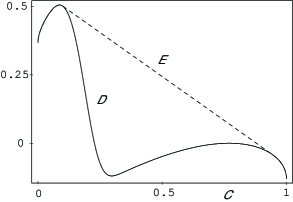
Figure 8: The quasispecies example (56), with $\gamma=5.$, and $\mu=1$, $\nu=0.3$. Left: The fitness function, $r=b-d$. Right: The function $e$ (solid line) and its concave envelope $\hat{e}$ (dashed), where it deviates from $e$.

8.1.2 Connection to the parallel model. The quasispecies model is closely related to the lumped parallel sequence space model with birth rates $B_{i}$, death rates $D_{i}$, and mutation rates $U_{i,i+1}=\mu(1-i/N)$, $U_{i,i-1}=\nu\,i/N$ and $U_{ij}=0$ for $\lvert j-i\rvert>1$ (where $\mu$ and $\nu$ are now mutation rates per site rather than probabilities). In fact, the latter may be considered as the former’s weak-selection weak-mutation limit (cf. [5, Ch.II.1.2], and [19]). It leads to the simpler expression

$$e(z)=b(z)-d(z)-g(z),$$ (57)

cf. (43), and [3, 18]. Indeed, this function is easily identified as the weak-selection weak-mutation limit of (55) by replacing $b$ by $1+\delta b$, $d$ by $1+\delta d$, $\mu$ by $\mu\delta$, $\nu$ by $\nu\delta$, and $e$ by $e/\delta$; the last replacement means that time is measured in units of $\delta$. $e(z)$ of (57) then emerges from (55) in the limit $\delta\to 0$.

8.2 Proof

The proof of Thm. 8.1 consists in verifying the assumptions of Thms. 7.1, 7.2 and 7.3 for the matrices $\boldsymbol{E}$ and $\boldsymbol{F}$ in (51)–(53). The main difficulty will be to establish the $\mathcal{O}(1/N)$ approximation as required in (A1). Besides the approximating function $e$ in (55) for $\boldsymbol{E}$, the approximating functions $f_{k}$ for $\boldsymbol{F}$ will be given by

$$f_{0}(z):=b(z)\big{(}p_{0}(z)-{\rm e}^{-g(z)}\big{)},\quad f_{k}(z):=b(z)\sqrt{p_{k}(z)p_{-k}(z)}\quad(0\neq k\in\mathbb{Z}),$$ (58)

where

$$p_{k}(z):=(\text{\rm Poi}_{\mu(1-z)}\ast\widehat{\text{\rm Poi}}_{\nu z})(k),\;k\in\mathbb{Z}.$$ (59)

These functions are quite natural, as they are obtained by replacing the binomial distributions at hand by their Poisson approximations. Nevertheless, the required approximation result is not at all automatic: Although $\text{\rm Bin}_{\mu,(N-i)/N}$ and $\widehat{\text{\rm Bin}}_{\nu,i/N}$ deviate from $\text{\rm Poi}_{\mu(N-i)/N}$ and $\widehat{\text{\rm Poi}}_{\nu i/N}$, respectively, by $\mathcal{O}(1/N)$ in variational distance [29, Section II.5], and this carries over to the convolution, it remains to be shown that the corresponding symmetrized quantities share this property. The key to this task is the fact that the Poisson distributions are particularly well-suited for a geometric symmetrization as in (51). This is the content of the following lemma.

Lemma 1

For $a,b\geq 0$, let $p_{\bullet}(a,b)=(p_{k}(a,b))_{k\in\mathbb{Z}}:=\text{\rm Poi}_{a}\ast\widehat{\text{\rm Poi}}_{b}$ be the convolution of the parameter-$a$ Poisson distribution with the reflected parameter-$b$ Poisson distribution. Then

$$\sqrt{p_{k}(a,b)p_{-k}(a,b)}={\rm e}^{-(\sqrt{a}-\sqrt{b})^{2}}\;p_{k}(\sqrt{ab},\sqrt{ab})$$

for all $k\in\mathbb{Z}$.

Proof

Since $p_{k}(a,0)=0$ for $k<0$, and $p_{k}(0,b)=0$ for $k>0$, the conclusion is immediate if either $a$ or $b$ vanishes. For $a,b>0$, the explicit formula

$$p_{k}(a,b)={\rm e}^{-a-b}\sum_{\begin{subarray}{c}\ell,m\geq 0:\\ \ell-m=k\end{subarray}}\frac{a^{\ell}b^{m}}{\ell!m!}$$ (60)

readily implies that $p_{-k}(a,b)=p_{k}(a,b)(b/a)^{k}$, whence

$$\sqrt{p_{k}(a,b)p_{-k}(a,b)}=p_{k}(a,b)(b/a)^{k/2}$$ (61)

for all $k\in\mathbb{Z}$. Inserting (60) into the last term and comparing the result with the similar expression for $p_{k}(\sqrt{ab},\sqrt{ab})$ we obtain the conclusion of the lemma.

We will be particularly interested in the Poisson approximation to the right-hand side of (49), viz.

$$p_{k}(z):=p_{k}(\mu(1-z),\nu z)\,,$$ (62)

where $z:=i/N$. Lemma 1 then implies that

$$\sum_{k\in\mathbb{Z}}\sqrt{p_{k}(z)p_{-k}(z)}={\rm e}^{-g(z)}\,,$$ (63)

thereby explaining the origin of the function $g$ defined in (54). We will also need the following tail estimate.

Lemma 2

For all $a,b\geq 0$,

$$\sum_{k\in\mathbb{Z}:\,|k|\geq\sqrt{N}}\sqrt{p_{k}(a,b)p_{-k}(a,b)}\leq\frac{2\sqrt{ab}}{N}\,.$$

Proof

If $a=0$ or $b=0$, $p_{k}(a,b)p_{-k}(a,b)=0$ except for $k=0$, so that the assertion is trivial. For $a,b>0$ we can write, using Lemma 1 and Markov’s inequality:

$$N\sum_{k\in\mathbb{Z}:\,|k|\geq\sqrt{N}}\sqrt{p_{k}(a,b)p_{-k}(a,b)}\leq\sum_{k\in\mathbb{Z}}k^{2}\,p_{k}(\sqrt{ab},\sqrt{ab})\,.$$

By symmetry, the last sum is the variance of $\text{\rm Poi}_{\sqrt{ab}}\ast\widehat{\text{\rm Poi}}_{\sqrt{ab}}$ and thus equal to $2\sqrt{ab}$.

We need a similar tail estimate for the geometric symmetrization of the matrix $\boldsymbol{P}$ defined in (50). Note that $\boldsymbol{P}$ depends on $N$.

Lemma 3

For all $i\in S$,

$$\sum_{j\in S:\,|j-i|\geq\sqrt{N}}\sqrt{P_{ij}P_{ji}}\leq\frac{C}{N}$$

for a constant $C$ depending on $\mu$ and $\nu$ but not on $N$.

Proof

We use the obvious inequality

$$\text{\rm Bin}_{n,p}(\ell)=(1-p)^{n}{n\choose\ell}\Big{(}\frac{p}{1-p}\Big{)}^{\ell}\leq{\rm e}^{a-np}\,\text{\rm Poi}_{a}(\ell)$$ (64)

which holds whenever $0\leq\ell\leq n$, $0<p<1$, and $a\geq np/(1-p)$. This implies that $P_{i,i+k}\leq{\rm e}^{a+b}\,p_{k}(a,b)$ with $a:=\mu/(1-v)$, $b:=\nu/(1-w)$, uniformly in $i\in S$. Hence

$$\sqrt{P_{i,i+k}P_{i+k,i}}\leq{\rm e}^{a+b}\,\sqrt{p_{k}(a,b)p_{-k}(a,b)}\,,$$ (65)

and the result follows from Lemma 2.

The crucial step is the following Poisson approximation of the geometric symmetrization of $\boldsymbol{P}$.

Proposition 4

With the abbreviation $p_{k}(z):=p_{k}(\mu(1-z),\nu z)$, we have

$$\sum_{j\in S}\Big{|}\sqrt{P_{ij}P_{ji}}-\sqrt{p_{j-i}(i/N)p_{i-j}(i/N)}\Big{|}=\mathcal{O}\Big{(}\text{\small$\frac{1}{N}$}\Big{)}$$ (66)

uniformly in $i$ as long as $i/N$ is bounded away from $0$ and $1$.

Proof

Consider an arbitrary $i\in S$ and suppose $z:=i/N$ is bounded away from $0$ and $1$. (We will generally suppress the $i$-dependence of all abbreviations to be introduced below.) The main difficulty of the proof comes from the fact that the parameters of the probabilities $P_{ji}$ depend on the variable $j$ rather than $i$. Fortunately, $\boldsymbol{P}$ is reversible, and Lemmas 2 and 3 allow us to confine ourselves to the $j$’s with $|j-i|\leq\sqrt{N}$. We proceed by a comparison of upper and lower bounds on

$$r_{k}:=\sqrt{P_{i,i+k}P_{i+k,i}}\,,\quad k\in S-i\,.$$

Step 1: A lower estimate. Since $\boldsymbol{P}$ is reversible w.r.t. $\text{\rm Bin}_{N,v/(v+w)}$, we have

$$r_{k}=P_{i,i+k}\sqrt{\frac{(i+k)!(N-i-k)!}{i!(N-i)!}}\Big{(}\sqrt{\frac{w}{v}}\Big{)}^{k}$$

for all $k\in S-i$. Since also $m!/n!\geq n^{m-n}$ for all $m,n$, it follows that

$$r_{k}\geq\underline{r}_{k}:=P_{i,i+k}\,s^{k}$$ (67)

for all $k$, where $s:=(iw/(N-i)v)^{1/2}=(z\nu/(1-z)\mu)^{1/2}$.

We now take the sum over $k$. Using (50) and the binomial formula we can write

$$\begin{split}\sum_{k\in S-i}\underline{r}_{k}&=(1-v+vs)^{N-i}(1-w+w/s)^{i}\\ \geq\;&\exp\big{(}-\mu(1-s)(1-z)\big{)}\Big{(}1-\frac{\mu^{2}(1-s)^{2}(1-z)^{2}}{N-i}\Big{)}\\ &\times\exp\big{(}-\nu(1-1/s)z\,\big{)}\Big{(}1-\frac{\nu^{2}(1-1/s)^{2}z^{2}}{i}\Big{)}\\ =\;&{\rm e}^{-g(z)}+\mathcal{O}\Big{(}\text{\small$\frac{1}{N}$}\Big{)}\,.\end{split}$$ (68)

The inequality follows from the fact that

$$\Big{(}1-\frac{x}{n}\Big{)}^{n}\geq{\rm e}^{-x}\Big{(}1-\frac{x^{2}}{n}\Big{)}$$ (69)

for any $n\geq 1$ and $\lvert x\rvert\leq n$; see [31, 3.6.2., p. 266]. In the last step we used that $z$ is bounded away from $0$ and $1$.

Step 2. An upper bound. Arguing as for (67) we find

$$r_{k}\leq P_{i,i+k}\Big{(}\frac{(i+k)w}{(N-i-k)v}\Big{)}^{k/2}=P_{i,i+k}\,s^{k}\,\big{(}\psi(k/N)\big{)}^{k}\,,$$

where $\psi(x):=(1+x/z)^{1/2}(1-x/(1-z))^{-1/2}$. Next, for each $k$ an expansion of $\psi$ gives

$$\big{(}\psi({k}/N)\big{)}^{k}=1+\frac{k^{2}}{N}\;\big{(}\psi(\vartheta_{k})\big{)}^{k-1}\psi^{\prime}(\vartheta_{k})$$

for some $\vartheta_{k}$ between $0$ and $k/N$. As long as $z$ is bounded away from $0$ and $1$ and $|k|\leq\sqrt{N}$, the $\psi$- and $\psi^{\prime}$-expressions on the right-hand side are bounded from above, so that

$$\big{(}\psi({k}/N)\big{)}^{k}\leq 1+\frac{k^{2}\,c^{k}}{N}$$

for some $c<\infty$. Also, using (64) we find

$$P_{i,i+k}\leq{\rm e}^{va+wb}\,p_{k}(a,b)\quad\text{ with }\quad a:=\frac{(N-i)v}{1-v},\;b:=\frac{iw}{1-w}\,.$$ (70)

Collecting all estimates we arrive at the upper bound

$$r_{k}\leq\bar{r}_{k}:={\rm e}^{va+wb}\,p_{k}(a,b)s^{k}\,\Big{(}1+\frac{k^{2}\,c^{k}}{N}\Big{)}\,.$$ (71)

Next, a summation over $k$ gives

$$\sum_{|k|\leq\sqrt{N}}\bar{r}_{k}\leq{\rm e}^{va+wb}\,\Big{(}\sum_{k\in\mathbb{Z}}p_{k}(a,b)s^{k}+\frac{K}{N}\Big{)}$$

with $K:=\sum_{k\in\mathbb{Z}}k^{2}\,(cs)^{k}\,p_{k}(a,b)$. To deal with the terms on the right-hand side we note first that $p_{k}(a,b)\,s^{k}={\rm e}^{as+b/s-a-b}p_{k}(as,b/s)$ by formula (60). Hence

$$\sum_{k\in\mathbb{Z}}p_{k}(a,b)\,s^{k}=\exp(as+b/s-a-b)=\exp\big{(}-g(z)\big{)}+\mathcal{O}\Big{(}\text{\small$\frac{1}{N}$}\Big{)}$$

because $a\approx(1-z)\mu$ and $b\approx z\nu$ up to error terms of order $1/N$. Likewise,

$$K=\exp\big{(}acs+b/(cs)-a-b\big{)}\sum_{k\in\mathbb{Z}}k^{2}\,p_{k}\big{(}acs,b/(cs)\big{)}$$

is bounded in $N$ since so are $a,b$. Since also $va+wb=\mathcal{O}(1/N)$, we finally arrive at the estimate

$$\sum_{|k|\leq\sqrt{N}}\bar{r}_{k}\leq{\rm e}^{-g(z)}+\mathcal{O}\Big{(}\text{\small$\frac{1}{N}$}\Big{)}\,.$$ (72)

Step 3: Conclusion. Consider now $q_{k}:=\sqrt{p_{k}(z)p_{-k}(z)}$. By (61), $q_{k}=p_{k}(z)s^{k}$. It is also immediate that $p_{k}(z)\leq{\rm e}^{va+wb}\,p_{k}(a,b)$ with $a,b$ as in (70). Hence $q_{k}\leq\bar{r}_{k}$ for all $k$. Combining this with Lemmas 2 and 3 and the bounds (67) and (71) we find

$$\begin{split}\sum_{k\in S-i}\lvert r_{k}-q_{k}\rvert&=\sum_{k\in S-i}\big{(}2\max(r_{k},q_{k})-r_{k}-q_{k}\big{)}\\ &\leq\mathcal{O}\Big{(}\text{\small$\frac{1}{N}$}\Big{)}+2\sum_{|k|\leq\sqrt{N}}\bar{r}_{k}-\sum_{k\in S-i}\underline{r}_{k}-\sum_{|k|\leq\sqrt{N}}q_{k}\,.\end{split}$$

Now, (68) and (72) show that the first sum exceeds the second only by a term of order $1/N$, and (72) together with (63) and Lemma 2 imply that the first sum exceeds the third by at most a term of order $1/N$. This completes the proof.

Besides the preceding key approximation in the interior of $\mathsf{D}$, we also need a uniform bound which will be used close to the boundary of $\mathsf{D}$. Here, an error bound of order $1/\sqrt{N}$ is sufficient.

Proposition 5

For all $i\in S$,

$$\sum_{j\in S}\sqrt{P_{ij}P_{ji}}\leq{\rm e}^{-g(i/N)}+\,\mathcal{O}\Big{(}\text{\small$\frac{1}{\sqrt{N}}$}\Big{)},$$

where the $\mathcal{O}(1/\sqrt{N})$ term depends on $\mu$ and $\nu$ but not on $i$.

Proof

In view of Lemma 3, we only need to estimate the sum over all $j=i+k\in S$ with $|k|\leq\sqrt{N}$. For these $j$ we find, using the Poisson bound (64) and writing again $z=i/N$,

$$\sqrt{P_{i,i+k}P_{i+k,i}}\leq{\rm e}^{\tilde{a}+\tilde{b}}\,\sqrt{p_{k}(a,b)p_{-k}(a,b)}.$$

Here $a=\mu(1-z+{1}/{\sqrt{N}})/(1-v)$, $b=\nu(z+{1}/{\sqrt{N}})/(1-w)$, and

$$\begin{split}\tilde{a}&=a-\mu(1-z-1/\sqrt{N})=2\mu/\sqrt{N}+\mathcal{O}(1/N)\,,\\ \tilde{b}&=b-\nu(z-1/\sqrt{N})=2\nu/\sqrt{N}+\mathcal{O}(1/N)\,,\end{split}$$

so that ${\rm e}^{\tilde{a}+\tilde{b}}=1+\mathcal{O}(1/\sqrt{N})$; the error terms do not depend on $i$. The claim thus follows from Lemmas 3, 2, 1 and the fact that $(\sqrt{a}-\sqrt{b})^{2}=g(z)+\mathcal{O}(1/\sqrt{N})$.

After these preparations we are now ready to read off the approximating functions $e$ and $f_{k}$ for the lumped quasispecies model, that is, we can proceed to the

Proof (of Thm. 8.1)

The main point of the proof is to establish condition (A1) for any compact interval $\mathsf{A}\subset\,]0,1[$. The (asymptotic) boundedness of the $B_{j}$’s and Lemma 3 imply that, for each $i\in S$,

$$\sum_{k\in S-i}\sqrt{B_{i}B_{i+k}P_{i,i+k}P_{i+k,i}}=\mathcal{O}\Big{(}\text{\small$\frac{1}{N}$}\Big{)}+\sum_{\lvert k\rvert\leq\sqrt{N}}\sqrt{B_{i}B_{i+k}P_{i,i+k}P_{i+k,i}}\,.$$ (73)

The asymptotics of the $B_{j}$’s implies further that the sum on the right-hand side is equal to

$$\Big{(}1+\mathcal{O}\Big{(}\text{\small$\frac{1}{N}$}\Big{)}\Big{)}\;b(z)\sum_{\lvert k\rvert\leq\sqrt{N}}\exp\big{(}\beta(z+k/N)-\beta(z)\big{)}\sqrt{P_{i,i+k}P_{i+k,i}}\,,$$ (74)

where $z:=i/N$ and $\beta(x):=(\log b(x))/2$. By hypothesis, $\beta\in C^{2}_{b}([0,1])$. Hence $\beta(z+k/N)-\beta(z)=\beta^{\prime}(z)k/N+\mathcal{O}(1/N)$ for $|k|\leq\sqrt{N}$, so that the last expression takes the form

$$\Big{(}1+\mathcal{O}\Big{(}\text{\small$\frac{1}{N}$}\Big{)}\Big{)}\;b(z)\sum_{\lvert k\rvert\leq\sqrt{N}}{\rm e}^{k\delta/N}\sqrt{P_{i,i+k}P_{i+k,i}}\,,$$ (75)

where $\delta:=\beta^{\prime}(z)$. Next we can omit the exponential ${\rm e}^{k\delta/N}$, making an error of order $1/N$ only. Indeed, using inequality (65) together with Lemma 1 and setting $a:=\mu/(1-v)$, $b:=\nu/(1-w)$ we obtain

$$\begin{split}\sum_{k\in S-i}\lvert{\rm e}^{k\delta/N}-1\rvert&\sqrt{P_{i,i+k}P_{i+k,i}}\\ &\leq{\rm e}^{a+b}\sum_{k\in\mathbb{Z}}\big{(}{\rm e}^{|k||\delta|/N}-1\big{)}\,p_{k}(\sqrt{ab},\sqrt{ab})\\ &\leq{\rm e}^{a+b}\Big{(}\exp\big{[}2\sqrt{ab}\,({\rm e}^{|\delta|/N}-1)\big{]}-1\Big{)}=\mathcal{O}\Big{(}\text{\small$\frac{1}{N}$}\Big{)}\,.\end{split}$$ (76)

The second inequality is obtained by taking formula (60) for $p_{k}(\sqrt{ab},\sqrt{ab})$, using ${\rm e}^{|k||\delta|/N}\leq{\rm e}^{\ell|\delta|/N}{\rm e}^{m|\delta|/N}$, and summing up. If $z=i/N$ is bounded away from $0$ and $1$, we can finally apply Prop. 4, Lemma 2 and the identity (63) to obtain

$$\begin{split}&\sum_{k\in S-i}\sqrt{B_{i}B_{i+k}P_{i,i+k}P_{i+k,i}}\\ &\qquad=\mathcal{O}\Big{(}\text{\small$\frac{1}{N}$}\Big{)}+\Big{(}1+\mathcal{O}\Big{(}\text{\small$\frac{1}{N}$}\Big{)}\Big{)}\;b(z)\sum_{\lvert k\rvert\leq\sqrt{N}}\sqrt{p_{k}(z)p_{-k}(z)}\\ &\qquad=b(z){\rm e}^{-g(z)}+\mathcal{O}\Big{(}\text{\small$\frac{1}{N}$}\Big{)}\,.\end{split}$$ (77)

Taking this together with the assumed approximation of the $D_{i}$, we arrive at the approximation (A1) of $\boldsymbol{E}$, and the diagonal elements of $\boldsymbol{F}$, by the functions $e$ and $f_{k}$ defined in (55) and (58). But the approximation of the nondiagonal elements of $\boldsymbol{F}$ is also guaranteed, since the estimates leading to (77) all hold term by term. This completes the proof of (A1).

Next, condition (A2) follows directly from Lemma 1 and the fact that Poisson distributions and their convolutions have a finite third moment. We note further that the upper bound on $F_{ij}$ and the lower bound on $E_{i}$ in (A3) and (A3^′) are obvious.

Before turning to the upper bound on $E_{i}$ let us discuss the particular context of Theorems 7.1, 7.2 and 7.3. We observe that the function $g$ is continuous on $[0,1]$ and smooth on $]0,1[$ with $g^{\prime}(0)=-g^{\prime}(1)=-\infty$, while $b>0$ and $d$ are $C^{2}$ functions on $[0,1]$. This entails that $e$ is $C^{2}$ on $]0,1[$ and attains its absolute maximum at a point $z^{*}\in\>]0,1[$; in particular, $z^{*}$ is contained in an interval $\mathsf{A}$ satisfying (A1) and (A2), as is required for Thm. 7.1. In addition, $e^{\prime\prime}$ is negative in a neigbourhood of $0$ and $1$, and has only finitely many zeroes by assumption. This implies that each basin of $e$ is determined by smooth hills, as is necessary for applying Thm. 7.3.

Now let $\mathsf{A}^{\prime}$ be any set of exposed smoothness points of $e$ which is bounded away from $0$ and $1$. If $\delta>0$ is sufficiently small, the set $\mathsf{A}_{\delta}^{\prime}$ of all $y$ satisfying $e(y)\geq t_{z}(y)-\delta$ for all $z\in\mathsf{A}^{\prime}$ is still bounded away from $0$ and $1$. For all $i$ with $i/N\in\mathsf{A}_{\delta}^{\prime}$, the upper bound on $E_{i}$ in (A3^′) follows directly from (77). For all other $i$’s, this bound follows from (73)–(76) as soon as $N$ is so large that the $\mathcal{O}(1/\sqrt{N})$-term in Prop. 5 is less than $\delta/\max b$. This completes the proof of (A3^′) under the conditions of Thms. 7.2 and 7.3. Since $]0,1[$ splits into finitely many intervals forming basins and smooth hills of $e$, the stated approximation result for $\Lambda$ follows. Finally, as $z^{*}$ is also an exposed point, the choice $\mathsf{A}^{\prime}=\{z^{*}\}$ gives us the upper bound on $E_{i}$ in (A3). Thm. 7.1 can therefore be applied, proving the approximation of $\lambda$ as stated.

- [1] E. Akin: The Geometry of Population Genetics. Springer, Berlin, 1979.
- [2] K. B. Athreya, P. E. Ney: Branching Processes. Springer, New York, 1972.
- [3] E. Baake, M. Baake, A. Bovier, M. Klein: An asymptotic maximum principle for essentially nonlinear evolution models. J. Math. Biol. 50, 83–114 (2005); ArXiv:q-bio.PE/0311020
- [4] E. Baake, H. Wagner: Mutation-selection models solved exactly with methods from statistical mechanics. Genet. Res. 78 93–117 (2001)
- [5] R. Bürger: The Mathematical Theory of Selection, Recombination, and Mutation. Wiley, Chichester, 2000
- [6] J. F. Crow, M. Kimura: An Introduction to Population Genetics Theory. Harper & Row, New York, 1970
- [7] A. Dembo, O. Zeitouni: Large Deviations: Techniques and Applications. Springer, New York, 1998
- [8] A. Edwards: The fundamental theorem of natural selection. Theor. Pop. Biol. 61, 335–337 (2002)
- [9] M. Eigen: Selforganization of matter and the evolution of biological macromolecules. Naturwiss. 58, 465–523 (1971)
- [10] M. Eigen, J. McCaskill, P. Schuster: The molecular quasi-species. Adv. Chem. Phys. 75, 149–263 (1989)
- [11] W. Ewens: Mathematical Population Genetics. Springer, Berlin, 2nd ed., 2004
- [12] W. Ewens, G. Grant: Statistical Methods in Bioinformatics. Springer, New York, 2nd ed., 2005
- [13] T. Garske: Error thresholds in a mutation-selection model with Hopfield-type fitness. Bull. Math. Biol., in press, arXiv:q-bio.PE/0505056; doi 10.1007/s11538-006-9072-1.
- [14] T. Garske, U. Grimm: A maximum principle for the mutation-selection equilibrium of nucleotide sequences. Bull. Math. Biol. 66, 397–421 (2004); arXiv:physics/0303053v2
- [15] H.-O. Georgii, E. Baake: Multitype branching processes: the ancestral types of typical individuals. Adv. Appl. Prob. 35, 1090–1110 (2003); arXiv:math.PR/0302049
- [16] U. Gerland, T. Hwa: On the selection and evolution of regulatory DNA motifs. J. Mol. Evol. 55 386–400 (2002)
- [17] J. Hein, M. Schierup, C. Wiuf: Gene genealogies, variation and evolution : a primer in coalescent theory. Oxford University Press, Oxford, 2005
- [18] J. Hermisson, O. Redner, H. Wagner, E. Baake: Mutation-selection balance: Ancestry, load, and maximum principle. Theor. Pop. Biol. 62, 9–46 (2002); arXiv:cond-mat/0202432
- [19] J. Hofbauer: The selection mutation equation. J. Math. Biol. 23, 41–53 (1985)
- [20] F. den Hollander: Large Deviations, AMS, Providence, RI, 2000
- [21] P. Jagers, O. Nerman: The stable doubly infinite pedigree process of supercritical branching populations. Zeitschrift für Wahrscheinlichkeitstheorie und verwandte Gebiete 65, 445-460 (1984)
- [22] P. Jagers: General branching processes as Markov fields. Stoch. Proc. Appl. 32, 183–242 (1989)
- [23] P. Jagers: Stabilities and instabilities in population dynamics. J. Appl. Prob. 29, 770–780 (1992)
- [24] C. Kamp: A quasispecies approach to viral evolution in the context of an adaptive immune system. Microbes and Infection 5, 1397–1405 (2003)
- [25] K. S. Karlin, H. M. Taylor: A first course in stochastic processes. Academic Press, San Diego, CA, 2nd edition, 1975
- [26] J. G. Kemeny, J. L. Snell: Finite Markov Chains. Springer, New York, 1981
- [27] H. Kesten, B. P. Stigum: A limit theorem for multidimensional Galton-Watson processes. Ann. Math. Statist. 37, 1211–1233 (1966)
- [28] T. Kurtz, R. Lyons, R. Pemantle, Y. Peres: A conceptual proof of the Kesten-Stigum theorem for multi-type branching processes. In K. B. Athreya, P. Jagers, eds, Classical and Modern Branching Processes, pp. 181–185, Springer, New York, 1997
- [29] T. Lindvall: Lectures on the Coupling Method. Wiley, New York, 1992
- [30] R. Lyons, R. Pemantle, Y. Peres: Conceptual proofs of LlogL criteria for mean behaviour of branching processes. Ann. Prob. 23, 1125–1138 (1995)
- [31] D. Mitrinovic: Analytic inequalities. Springer, Berlin, 1970
- [32] R. T. Rockafellar: Convex Analysis. Princeton University Press, Princeton, NJ, 1970
- [33] W. Stannat: On the convergence of genetic algorithms – a variational approach. Probab. Theory Relat. Fields 129, 113–132 (2004)