Manipulating single enzymes by an external harmonic force

Abstract

We study a Michaelis-Menten reaction for a single two-state enzyme molecule, whose transition rates between the two conformations are modulated by an harmonically oscillating external force. In particular, we obtain a range of optimal driving frequencies for changing the conformation of the enzyme thereby controlling the enzymatic activity (i.e. product formation). This analysis demonstrates that it is, in principle, possible to obtain information about particular rates within the kinetic scheme.

Recent advances in single molecule spectroscopy have made it possible to follow the catalytic activity of individual enzymes over extended periods of time edman00 ; schenter99 ; english06 ; kou05 ; flomenbom05 ; lerch05 . Although the catalytic rates have been shown to be distributed in time, the general Michaelis-Menten scheme, originally proposed for an ensemble of enzymes, turned out to hold quite well also on the level of a single enzyme edman00 ; schenter99 ; english06 ; kou05 ; flomenbom05 ; lerch05 ; min06 ; xue06 . What is still left open is the nature of the conformational changes and its relationship to the enzymatic activity lerch05 ; min06 ; xue06 ; flomenbom06 . Deeper insights into the conformational-activity relationship can be obtained by influencing single enzyme conformations by an external force and following the effects on the catalytic activity. The possibility to manipulate enzymatic turnovers by applying a mechanical force has been recently demonstrated in wiita06 . Also, voltage-gated ion channels can be manipulated electrically to switch between two states pustovoit06 . Here, assuming a two-state Michaelis-Menten scheme for a single enzyme, we investigate how one can manipulate the activity (turnovers) of an enzyme by an external harmonic force. The oscillatory force is shown to be able to increase the weight (occurrence time) of a desired conformation in the scheme, controlling the enzyme activity.

Figure 1: Michaelis-Menten scheme for a single enzyme with two conformations. E denotes the enzyme molecule, S the substrate, and P the product. Rates $\alpha_{ij}$ and $\beta_{ij}$ ($i,j=1,2$) stand for transitions between conformational states 1 and 2, while rates $k_{xi}$ ($x=-1,1,2$) quantify internal conversions.

The reaction scheme that we examine is shown in Fig. 1. We model the effect of the time-dependent external force as a shift in the conformational energy landscape. Assuming that the transitions between different conformations, with rates $\alpha_{ij}$ and $\beta_{ij}$, follow an Arrhenius activation, and using a harmonic force which modulates barriers separating conformational states, we find the following time dependence of the rates

$$\alpha_{ij} = \alpha_{ij}(t)=\alpha_{ij}^{(0)}\exp\left(-\epsilon_{ij}^{(\alpha)}\sin(\omega t+\phi_{0})\right),$$ (1a)

$$\beta_{ij} = \beta_{ij}(t)=\beta_{ij}^{(0)}\exp\left(-\epsilon_{ij}^{(\beta)}\sin(\omega t+\phi_{0})\right).$$ (1b)

Here, $\omega$ is the angular frequency of the external driving force, $\phi_{0}$ the initial phase of the force; and $\alpha_{ij}^{(0)}$, $\beta_{ij}^{(0)}$, $\epsilon_{ij}^{(\alpha)}$, and $\epsilon_{ij}^{(\beta)}$ are phenomenological constants characterizing the enzyme and the amplitude of the driving force. In Eqs. (1) we assume that the potential energy landscape of the conformations responds instantly to changes in the force. This assumption can be relaxed, for instance by including different phases $\phi_{0}$ for $\alpha_{ij}$ and $\beta_{ij}$. Note, however, that a $180^{\circ}$ phase difference, corresponding to a change of sign for $\epsilon_{ij}^{(\beta)}$, is included in Eqs. (1). We assume that the substrate S is in great excess, such that the rates for the reaction with the substrate like $k_{1i}=k_{1i}^{(0)}[{\rm S}]$ become independent of time. The scheme in Fig. 1 is closely related to schemes describing resonant activation in discrete systems flomenbom04 .

Simulations. As shown below, for certain limits of the rates analytical expressions can be derived. To obtain insight into the general behavior of enzymatic activity including noise, we use a stochastic simulation. To this end, we implemented the Gillespie algorithm gillespie , that provides random values for the waiting time between two reaction steps, and the direction of the reaction as weighted by the corresponding Arrhenius factor. We start the system in one of the states ${\rm E}_{i}+{\rm S}$, and then perform jumps to one of the neighboring states according to the Gillespie reaction probability. Which state it jumps to is decided by picking a waiting time for jumping to state ${\rm ES}_{i}$ according to the exponential distribution with rate parameter $k_{1i}$, and one for jumping to ${\rm E}_{j}+{\rm S}$ according to the cumulative distribution

$$F_{\alpha_{ij}}(\Delta t)=1-\exp\left(-\int_{t}^{t+\Delta t}\alpha_{ij}(t^{\prime})dt^{\prime}\right),$$ (2)

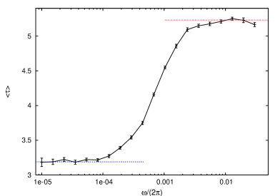
Figure 6: Plot of $\left<\tau\right>$ as function of driving frequency $\omega$ for $\alpha_{ij},\beta_{ij}\ll k_{xi}$. The horizontal lines represent the limits derived in the text. The parameters are $k_{1i}=k_{-1i}=1$, $k_{21}=0.3$, $k_{22}=3$, $\alpha_{12}^{(0)}=2\times 10^{-4}$, $\alpha_{21}^{(0)}=10^{-3}$, $\beta_{12}^{(0)}=2\times 10^{-5}$, $\beta_{21}^{(0)}=10^{-4}$, $\epsilon_{12}^{(\alpha)}=3$, $\epsilon_{21}^{(\alpha)}=-3$, $\epsilon_{12}^{(\beta)}=3$ and $\epsilon_{21}^{(\beta)}=-3$. The simulation comprises $2\times 10^{6}$ turnovers per frequency.

and then the jump is made to the state with the shortest waiting time. Subsequent jumps to neighboring states are determined similarly, and one iteration of the simulation stops at time $t=\tau$ when the system reaches one of the product states ${\rm E}_{i}+{\rm P}$. The conformation $i$ of the enzyme is then used as the initial state for the next iteration with the initial phase $\phi_{0}^{({\rm new})}=\omega\tau+\phi_{0}^{({\rm old})}$ determining the new momentary force. Performing iterations over many periods of the oscillating force we obtain a time series for the turnover times $\tau$, from which the average waiting time $\left<\tau\right>$ yields. Plots of $\left<\tau\right>$ as a function of $\omega$ are shown in Figs. 2 and 6. Depending on the choice of parameters, switching between two or three kinetic regimes of the system is revealed. Certain limiting behaviors are accessible analytically, as discussed soon. For the parameters used throughout this work the rate of product formation in the conformation 2 is higher than in conformation 1.

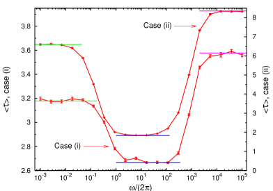
Figure 2: Mean turnover time $\left<\tau\right>$ as function of driving frequency $\omega$ for the case $k_{xi}\ll\alpha_{ij},\beta_{ij}$. Horizontal lines represent the limit cases derived in the text. (i) $k_{1i}=k_{-1i}=1$, $k_{21}=0.3$, $k_{22}=3$, $\alpha_{12}^{(0)}=80$, $\alpha_{21}^{(0)}=800$, $\beta_{12}^{(0)}=160$, $\beta_{21}^{(0)}=1600$, $\epsilon_{12}^{(\alpha)}=2=-\epsilon_{21}^{(\beta)}$, $\epsilon_{12}^{(\beta)}=3=-\epsilon_{21}^{(\alpha)}$. (ii) the following parameters were changed: $k_{11}=k_{-11}=k_{-12}=0.01$, $k_{12}=3=-\epsilon_{12}^{(\beta)}$, $\epsilon_{21}^{(\beta)}=2$ (units on right axis). Simulations were run for $5\times 10^{4}$ turnovers per frequency.

We note that in our analysis the parameters (except for case (ii) in Fig. 2) are chosen such that detailed balance is fulfilled, as required for certain single enzymes that are coupled to the surrounding heat bath gopich06 . The explicit condition arising when detailed balance is applied around the loop in the reversible reaction pathway in Fig. 1, is $k_{-11}\beta_{21}(t)k_{12}\alpha_{12}(t)=k_{11}\beta_{12}(t)k_{-12}\alpha_{21}(t)$. The condition is applied for any momentary value of the external force, and therefore any time $t$, since the system could equally well be held constantly at these forces. Detailed balance could be violated, for instance, by enzymes converting ATP energy during their cycle.

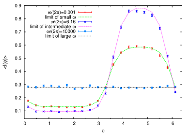
Figure 3: Plot of $\left<I(\phi)\right>$ as a function of $\phi$ for different driving frequencies $\omega$, for the same conditions as in Fig. 2 (i).

Fast switching limit. Consider the case when the switching between enzyme conformations is much faster than the reactions with the substrate, as displayed in Fig. 2. Note that case (ii) in Fig. 2 has different $k_{1i}$’s thefootnote . It also includes a $180^{\circ}$ shift in the phases of variation of rates $\alpha_{ij}$ and $\beta_{ij}$ under the external force distinguishing between substrate-bound and substrate-free enzyme states. Parameters were chosen to reflect situations with enhanced enzyme efficiency at intermediate frequencies. Different scenarios, for instance with decreased efficiency, are also possible. In both cases in Fig. 2 the rates satisfy $k_{xi}\ll\alpha_{ij},\beta_{ij}$. This means that we can define effective rates $k_{x}$ as averages over the various conformations. The weights in these averages are given by the probabilities for the enzyme to be in the different conformations. If $\omega$ is much faster or slower than the relaxation time between the two enzyme conformations, these probabilities can be easily obtained. For instance, the probability for the enzyme to be in conformation ${\rm E}_{1}$, given that no substrate is bound, is

$$p(1|E,\phi)=\left\{\begin{array}[]{ll}\alpha_{21}(\phi)/[\alpha_{12}(\phi)+\alpha_{21}(\phi)],&\omega\ll\alpha_{ij}\\[5.69046pt] {\bar{\alpha}}_{21}/[{\bar{\alpha}}_{12}+{\bar{\alpha}}_{21}],&\omega\gg\alpha_{ij}\end{array}\right.$$ (3)

where $\phi\in(0,2\pi)$ is the phase of the force, i.e., $\omega t+\phi_{0}=\phi+2\pi n$ for some integer $n$, and a bar over a quantity means that this quantity is averaged over all phases,

$${\bar{\alpha}}_{ij}=\int_{0}^{2\pi}\frac{d\phi}{2\pi}\alpha_{ij}(\phi)=\alpha_{ij}^{(0)}I_{0}\left(\epsilon_{ij}^{(\alpha)}\right),$$ (4)

where $I_{0}$ is the modified Bessel function of order 0. The effective rates $k_{x}$ can now be obtained in the two limits,

$$k_{x}(\phi)=\left\{\begin{array}[]{ll}\sum_{i}k_{xi}p(i|x,\phi),&\omega\ll k_{xi}\\[5.69046pt] \sum_{i}k_{xi}{\bar{p}}(i|x),&\omega\gg k_{xi}\end{array}\right.,$$ (5)

where $x$ in $p(i|x,\phi)$ refers to the unbound state ${\rm E}+{\rm S}$ for $x=1$, and to the bound state ${\rm ES}$ for $x=-1$ and $x=2$. The rate of the overall reaction is then given by the standard Michaelis-Menten expression kou05 ; english06 ; gopich06

$$\nu(\phi)=\frac{k_{2}(\phi)k_{1}(\phi)}{k_{1}(\phi)+k_{-1}(\phi)+k_{2}(\phi)}$$ (6)

as function of the phase $\phi$. The average waiting time $\left<\tau\right>$ for one turnover can now be found by averaging over all phases and calculate $\left<\tau\right>=1/{\bar{\nu}}$. The values of $\left<\tau\right>$ calculated according to Eqs. (5) and (6) are shown in Fig. 2 by the horizontal lines. We note that the limits where $\omega\ll\alpha_{ij},\beta_{ij}$ can also be obtained as limit cases of the system studied in Ref. astumian93 .

Another experimentally relevant quantity is the temporal probability density for the formation of products at a given value of the force as determined by the phase $\phi$. A plot of this intensity of product formation events, which we label by $\left<I(\phi)\right>$, is shown in Fig. 3. An approximate bimodal behavior is found for certain choices of the parameters. To obtain the analytic limits we note that if the external force is slowly varying, i.e., $\omega\ll k_{xi},\alpha_{ij},\beta_{ij}$, then the intensity will simply be equal to the rate $\left<I(\phi)\right>=\nu(\phi)$. This expression also holds for $\omega\gg\alpha_{ij},\beta_{ij}$ where it is independent of $\phi$. For the intermediate $\omega$ where $k_{xi}\ll\omega\ll\alpha_{ij},\beta_{ij}$ it will be the distribution of conformations in the final step of the reaction and the corresponding rate constants that determines when the product formation happens, such that $\left<I(\phi)\right>={\bar{\nu}}\sum_{i}k_{2i}p(i|{\rm ES},\phi)/{\bar{k}}_{2}$. We point out here that at slow frequencies it is the overall efficiency of the enzyme that is probed at different magnitudes of the external force, while at the intermediate frequencies it is only the relative efficiency of the final step in the reaction which is probed at different external driving. Thus tuning the frequency allows one to selectively study the final reaction step.

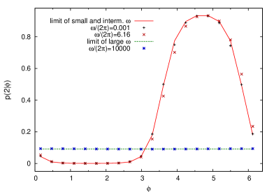
Figure 4: Estimate of $p(2|\phi)$ as a function of $\phi$ for the same parameters as in Fig. 2 (i). Note that there are only two different analytic limits, since two of the three limits are identical for the chosen parameters.

The behavior of $\left<I(\phi)\right>$ in Fig. 3 can be compared with the probability of being in, say, conformation 2 (the fast one) as a function of $\phi$, as shown in Fig. 4. Note the large change in amplitude for the chosen parameters. To obtain the analytic limits we write the probability as $p(i|\phi)=p(i|{\rm E},\phi)p({\rm E}|\phi)+p(i|{\rm ES},\phi)[1-p({\rm E}|\phi)]$, where $p(i|{\rm E},\phi)$ is given by Eq. (3). To find $p(E|\phi)$ note that at a given phase $\phi$ the effective rate for the system to leave the state without bound substrate is $k_{1}(\phi)$, and the rate for leaving the state with bound substrate is $k_{-1}(\phi)+k_{2}(\phi)$. In fact the quasi-steady-state probability for being in the state without bound substrate is

$$p(E|\phi)=\frac{k_{-1}(\phi)+k_{2}(\phi)}{k_{1}(\phi)+k_{-1}(\phi)+k_{2}(\phi)}$$ (7)

in the two cases given by Eq. (5) where either $\omega\ll k_{xi}$ or $\omega\gg k_{xi}$. The resemblance of Figs. 3 and 4 reflects the dominating role of the conformation 2, due to its larger catalytic rate, in the enzymatic activity.

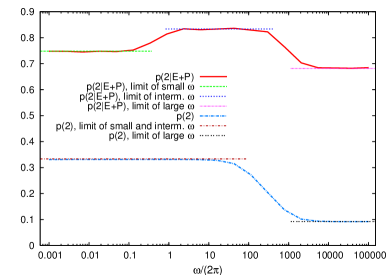
Figure 5: Plot of the fraction $p(2)$ the enzyme spends in conformation 2 (lower curve), as a function of driving frequency $\omega$ for the same parameters used in Fig. 2 (i). The upper curve depicts the fraction of product formation while the enzyme is in conformation 2.

To illustrate further the mechanisms behind the transitions of $\left<\tau\right>$ with changing driving frequency we plotted the fraction of time the enzyme spends in conformation 2, labeled $p(2)$, during a simulation run in Fig. 5. The analytic limits of $p(2)$ can be obtained straightforwardly by averaging the probability of being in conformation 2 over all phases, $p(i)=\int_{0}^{2\pi}[d\phi/(2\pi)]\;p(i|\phi)$. This behavior can be compared with the fraction of product formation events that occurs while the enzyme is in conformation 2, labeled by $p(2|E+P)$ in Fig. 5. The analytical limits of $p(2|E+P)$ can be obtained by averaging over all phases $\phi$ the effective rate constant for forming a product in conformation $i$, $k_{2i}p(i|{\rm ES},\phi)$, divided by the overall effective $k_{2}(\phi)$, taking into account the varying rate of product formation by a factor $\nu(\phi)/{\bar{\nu}}$. The explicit formula is

$$p(i|{\rm E+P})=\int_{0}^{2\pi}\frac{d\phi}{2\pi}\;\frac{k_{2i}p(i|{\rm ES},\phi)}{k_{2}(\phi)}\,\frac{\nu(\phi)}{{\bar{\nu}}}.$$ (8)

As Fig. 5 illustrates, the slowing down of the reaction with increasing frequency at the second transition in Fig. 2 occurs because the high frequency of the force shifts the enzyme towards spending more time in the low efficiency conformation. The increased efficiency of the enzyme at intermediate frequencies sets in when the external force drives the enzyme back and forth between its two conformations fast enough to avoid the bottleneck of the enzyme spending long uninterrupted periods being forced towards the slowly reacting conformation.

Slow switching limit. When the switching between enzyme states is slow in comparison to substrate reactions, $\alpha_{ij},\beta_{ij}\ll k_{xi}$, the enzyme will mostly stay in the same state during a reaction cycle, and we can therefore take the instantaneous reaction rate to be

$$\nu(\phi)=p(1|\phi)\nu_{1}+p(2|\phi)\nu_{2},$$ (9)

where $\nu_{i}=k_{2i}k_{1i}/(k_{1i}+k_{-1i}+k_{2i})$ are the fixed conformation rates and $p(i|\phi)$ is the probability for the enzyme to be in conformation $i$ at a given phase of the oscillating force. To find this probability we first argue in the same way as Eq. (7) was obtained to see that the (steady-state) probability of being in the state without bound substrate, given that the conformation is $i$, is

$$p(E|i)=\frac{k_{-1i}+k_{2i}}{k_{1i}+k_{-1i}+k_{2i}}\;.$$ (10)

Then we note that the effective rate constant for changing conformation from $i$ to $j$ can be found as

$$\gamma_{ij}=p(E|i)\alpha_{ij}+(1-p(E|i))\beta_{ij}.$$ (11)

This effective rate now allows the probability of being in conformation $i$ to be calculated similarly to Eq. (3) as

$$p(i|\phi)=\left\{\begin{array}[]{ll}\gamma_{ji}(\phi)/[\gamma_{ij}(\phi)+\gamma_{ji}(\phi)],&\omega\ll\gamma_{ij}\\ {\bar{\gamma}}_{ji}/[{\bar{\gamma}}_{ij}+{\bar{\gamma}}_{ji}],&\omega\gg\gamma_{ij}\end{array}\right.$$ (12)

where $j=3-i$. The averaged waiting time for one turnover can again be found as $\left<\tau\right>=1/{\bar{\nu}}$.

Discussion. Detailed knowledge of the dynamics of single enzymes as well as their response to external stimulus is important for the understanding of biochemical processes occurring in living cells. We studied the response of a single two-state enzyme to a harmonic external driving force in the presence of thermal noise. By combination of analytic and simulations results, we demonstrated the rich response behavior of the turnover dynamics of the enzyme to an external force. We showed that in some cases there exists optimum driving frequencies that minimize the turnover time of the enzyme. In these cases one can selectively obtain information on the reaction rates in the final step of the Michaelis-Menten reaction by choosing an oscillation in a suitable frequency range. Moreover, we found that the response of the enzyme activity can be very sensitive within a small range of phase $\phi$, a signature of many biological switches. We note that it should be possibly to access the full spectrum of relevant driving frequencies by combining different experimental methods, such as atomic force microscopy and optical switching methods.

MAL and RM acknowledge partial funding from the Natural Sciences and Engineering Research Council (NSERC) of Canada, and the Canada Research Chairs program. MU and JK acknowledge financial support from the Deutsche Forschungsgemeinschaft (HA 1517/26-1,2 Single molecules).

References

- (1) G. K. Schenter, H. P. Lu, and X. S. Xie, J. Phys. Chem. A 103, 10477 (1999).
- (2) L. Edman and R. Rigler, Proc. Natl. Acad. Sci. USA 97, 8266 (2000).
- (3) B. P. English, et al., Nat. Chem. Biol. 2, 87 (2006).
- (4) S. C. Kou, et al., J. Phys. Chem. B 109, 19068 (2005).
- (5) O. Flomenbom, et al., Proc. Natl. Acad. Sci. USA 102, 2368 (2005).
- (6) H. P. Lerch , R. Rigler , A. S. Mikhailov, Proc. Natl. Acad. Sci. USA 102, 10807 (2005).
- (7) W. Min, et al., J. Phys. Chem. B 110, 20093 (2006).
- (8) X. Xue, F. Liu, and Zh. Ou-Yang, Phys. Rev. E 74, 030902 (R) (2006).
- (9) O. Flomenbom and R. J. Silbey, Proc. Natl. Acad. Sci. USA 103, 10907 (2006).
- (10) V. A. P. Wiita, et al., Proc. Natl. Acad. Sci. USA 103, 7222 (2006).
- (11) M. A. Pustovoit, A. M. Berezhkovskii, and S. M. Bezrukov, J. Chem. Phys. 125, 194907 (2006).
- (12) O. Flomenbom and J. Klafter, Phys. Rev. E 69, 051109 (2004).
- (13) D. T. Gillespie, J. Comp. Phys. 22, 403 (1976).
- (14) I. V. Gopich and A. Szabo, J. Chem. Phys. 124, 154712 (2006).
- (15) In case (i) of Fig. 2 we kept in accordance with the experimental data english06 which indicate a difference between the values of only.
- (16) R. D. Astumian and B. Robertson, J. Am. Chem. Soc. 115, 11063 (1993).