Effect of supercoiling on formation of protein mediated DNA loops

Abstract

DNA loop formation is one of several mechanisms used by organisms to regulate genes. The free energy of forming a loop is an important factor in determining whether the associated gene is switched on or off. In this paper we use an elastic rod model of DNA to determine the free energy of forming short (50–100 basepair), protein mediated DNA loops. Superhelical stress in the DNA of living cells is a critical factor determining the energetics of loop formation, and we explicitly account for it in our calculations. The repressor protein itself is regarded as a rigid coupler; its geometry enters the problem through the boundary conditions it applies on the DNA. We show that a theory with these ingredients is sufficient to explain certain features observed in modulation of in vivo gene activity as a function of the distance between operator sites for the lac repressor. We also use our theory to make quantitative predictions for the dependence of looping on superhelical stress, which may be testable both in vivo and in single-molecule experiments such as the tethered particle assay and the magnetic bead assay.

I Introduction and summary

I.A Introduction

Many genetic processes in bacteria are controlled by proteins that bind at separate, often widely spaced, sites on DNA and hold the intervening double helix in a loop dunn84a ; adhy89a ; schl92a ; half04a . For example, the lactose metabolism system in E. coli is controlled by a repressor protein, LacI, binding to a set of binding sites. Early evidence for the existence of a looping mechanism came from the observation that the ability of a cell to control a particular gene depended in an approximately periodic way upon the number of basepairs of DNA intervening between two particular protein-binding sequences (called “operators”) (see for example dunn84a ; hoch86a ; kram87a ; bell88a ). Some recent data appear in Fig. 1. The periodic modulation was found to be roughly independent of the details of what basepair sequence was inserted or deleted between the operators; insertions and deletions elsewhere did not affect the gene regulation in this way.

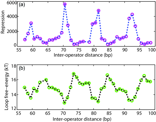
Figure 1: a. Repression of a gene product controlled by the lac repressor in E. coli cells. The data are from mull96a , Figure 3a; see that paper for an explanation of the units on the vertical axis. The horizontal axis gives the distance along the DNA between the centers of the two operators, each 21 basepairs long. In this paper we will express operator spacing by a number $L$ that equals this number minus 21bp (Fig. 2). Other experiments have obtained similar curves using operators located on a plasmid beck05a . b. Looping free energy inferred from the data in (a), showing a roughly periodic modulation with operator spacing (from saiz05a , Figure 3). The maxima of this function correspond to poor looping efficiency, that is, to the minima in panel (a). There is a slight minimum in the lower envelope of this function around 70–80bp, corresponding to our $L\approx 50$–60bp. A similar function emerges from the more detailed analysis of Garcia et al. garc?a .

The interpretation of these results followed an analogy to the related process of DNA cyclization. Suppose that a regulatory protein binds stereospecifically to the two operators, forcing them into close physical proximity, with the intervening DNA forming a loop (Fig. 2). The equilibrium constant for this isomerization reaction depends on the free energy change, which contains as a component the elastic energy cost of forming the loop. The elastic energy, in turn, contains terms reflecting bending and twisting deformation. For a favorable value of the interoperator spacing, loop formation involves only bending of the DNA. For spacing differing slightly from the optimum, however, bringing the loop ends into the relative orientation imposed by the protein complex requires an additional rotation of one end about its axis. The extra elastic energy cost entailed by this deformation reduces the equilibrium constant for loop formation relative to the optimal spacing. But if the spacing is increased by a full helical turn $L_{\rm helix}$ (about 11 basepairs), then we once again have a twist-free loop solution, a relatively low elastic energy cost, and hence a relatively high level of gene regulation. Thus the hypothesis of loop formation predicts a periodic modulation of the regulatory efficacy with loop size, as observed. Mossing and Record put forward a version of this theory shortly after the first experimental results moss86a .

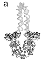
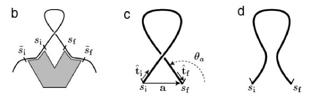
Figure 2: a. Crystallographically derived structure of the lac repressor (LacI, dark gray) bound to two operator segments of DNA (black) lewi96a . The light gray curve represents a DNA conformation interpolating between the operator segments, obtained in Ref. bala99a . b. Cartoon of the class of loops we will study. The DNA is considered free in the region between the two exit points $s_{\rm i}$ and $s_{\rm f}$. These exit points are located at $\pm 10.5\,$bp from the operator centers. Within the binding sites themselves, the protein may induce kinks in the DNA, as shown. c. Definition of the initial and final tangent vectors $\hat{\mathbf{t}}_{\rm i}$, $\hat{\mathbf{t}}_{\rm f}$, the separation vector $\mathbf{a}$, and the angle $\theta_{a}$ characterizing our idealized DNA–protein complex. $\mathbf{a}$ is the vector joining the two exit points, located at arclengths $s_{\rm i}$ and $s_{\rm f}$. The arclength separation between exit points is $L=s_{\rm f}-s_{\rm i}$. The vectors $\hat{\mathbf{t}}_{\rm i}$, $\hat{\mathbf{t}}_{\rm f}$, and $\mathbf{a}$ are all assumed to be be coplanar, and the angle $\theta_{a}$ from $\mathbf{a}$ to $-\hat{\mathbf{t}}_{\rm f}$ is equal to that from $-\mathbf{a}$ to $\hat{\mathbf{t}}_{\rm i}$ (the “planar, symmetric coupler” idealization). In the example shown, $\theta_{a}>90^{\circ}$. Although the coupler is planar, the loop itself will not in general be so, as illustrated here. d. The $\star$-loop configuration corresponding to (c) (see text Sect. III.C). This loop is always planar.

Later, looped DNA complexes similar to those inferred by the above argument were seen directly in electron microscopy (e.g. kram87a ) and other modalities. More recently, single-molecule experiments have demonstrated DNA looping in vitro, and enabled the systematic study of the looping reaction as a function of external parameters such as stretching force finz95a ; lia03a . On the structural side, advances in x-ray crystallography have yielded structures for the operator-protein complex, for example in the lac operon system lewi96a ; bell01a ; bell01b . Starting with that work, many authors have sought to determine the detailed form of the loop using physical modeling (see Sect. II.A). A more ambitious goal would be to predict the looping free energy function, which has recently been phenomenologically extracted from experimental studies of gene repression in vivo (for example bint05b ; saiz05a ; saiz?a ; garc?a ; see Fig. 1b). This paper is intended as a step in that direction.

I.B Goals of this work

Our goal in this paper is to introduce one important physical aspect of looping, relevant both in vivo and in single-molecule assays. This is the presence of significant torsional stress (supercoiling) in the region of DNA outside the loop-forming tract. Certainly everyday experience teaches that external torque can predispose an elastic rod (such as a garden hose) to form a loop.

A simple estimate shows that this external stress can significantly alter the equilibria between the unlooped state and various alternative looped states. As we will review later, bacteria maintain their chromosomal DNA in a negatively supercoiled (undertwisted) state, with a local torsional stress $M_{\rm ext}$ of about $-4\,$pN nm (see Sect. II.A.2). Formation of a loop can relax the external DNA by an angle on the order of $\pm\pi$ radians, allowing the external torsional stress to do work $\approx\pm\pi M_{\rm ext}\approx\pm 3\,{k_{\rm B}T}$ on the looping complex. This energy scale is comparable to the looping energies inferred from data (Fig. 1b), so we must account for it. Indeed, previous authors have already documented a large effect of supercoiling on a related process, the juxtaposition of sequentially distant points on a long circular DNA molecule klen95a ; volo96a . We wish to study similar effects in a simple way, in the context of DNA looping. Specifically, we will calculate, in a simplified model, the quasiperiodic dependence of the looping free energy (Fig. 1b) on the interoperator spacing $L$.

We also give a procedure to find, in an idealized physical model, the equilibrium shapes and energies of an elastic rod under the sort of end constraints appropriate to DNA loop formation by a protein complex. Our method uses the explicit analytic solutions to the elastic-rod equations, and hence enjoys significant computational advantages over gradient-descent algorithms.

Our results show that indeed external torque affects looping equilibria, and can change which of multiple looped states is most favorable. Specifically, the shape of the looping free energy curve reflects exchanges of stability as $L$ increases; the critical values of $L$ for these exchanges (local maxima of Fig. 1b) depend on the external torsional stress. These results can be tested, for example in vivo by studying bacteria with varying levels of supercoiling density (volobook , section 2.II.D), or in vitro by the methods of Lia et al. lia03a . The methods developed in this paper may also be applicable to other systems where DNA loops are implicated half04a .

The paper is organized as follows. Sect. II outlines some prior work and sets out the many simplifications we introduce to keep the treatment of external supercoiling relatively transparent. Sect. III gives more details of our calculation strategy. Sect. IV presents the actual calculation, and Sect. V discusses the results. Expert readers wishing to see the key new elements of our approach will find them in Sects. III.B–III.D and IV.B.

The Appendix gives a glossary of symbols used in the text.

II Physical framework

In the first subsection below we describe some of the physical ingredients that enter into the problem of modeling DNA looping. It is not possible to survey here the large literature on such models, but we will mention some of the prior work incorporating these ingredients. Mainly we discuss work on the lac system, but extensive work has also been done on other regulatory systems, such as gal (e.g. gean01a ) and lambda (e.g. bell00a ), and on the binding of nucleosomes to miniplasmids (e.g. tobi00a ).

II.A Ingredients of the problem and prior work

II.A.1 Loop structure

The crystallographic work of Lewis and coauthors gave only the structure of the regulatory protein complex bound to two short DNA segments containing the operators. Following this work, several authors used elastic models of DNA to propose structures for the complete looped state (for example, bala99a ; tsod99a ; tobi00a ; bala04a ; bala04b ; doua05a ; bala06a ). (Earlier authors studied similar mathematical problems in other contexts, for example, tobi94a ; cole95a ). The basic premise of these works is that the regulatory protein complex binds to two specific elements on the DNA, with a fixed, specified orientation relative to it (the “strong anchoring end condition” tobi00a ). The DNA between the two binding regions must accommodate to these constraints by adopting a form different from the one it would otherwise have taken; finding this form is a boundary-value problem in the elasticity of a slender body. These works included varying levels of realism in their treatment of the DNA elasticity: Some included bend anisotropy, sequence dependence, and electrostatic effects. Some, however, neglected DNA twist stiffness altogether, and so could not address the periodic phasing dependence that is part of our main motivation.

Several authors have recognized that there may be alternate DNA binding patterns, giving rise to multiple looping states (for example gean01a ; swig06b ; saiz?a ). We discuss this further in Sect. II.B.3 below.

In addition to purely elastic effects, it has long been recognized that the conformation of DNA is critically affected by chain entropy. An early calculation including these effects was Shimada and Yamakawa’s study of DNA cyclization, the formation of circular DNA from linear pieces; later work has extended and refined their results shim84a ; zhan03a ; spak06a . Recent work on DNA looping has begun to incorporate entropic corrections following a similar calculational approach zhan06a ; swig06b ; zhan? . Although these corrections can be significant, for short loops the strong anchoring condition constrains the DNA so much that elastic effects dominate over conformational entropy (at least for understanding the periodic phasing dependence that is our central concern).

Other calculations have acknowledged that the protein complex formed in DNA looping may not be a rigid object; stresses transmitted from the bent DNA may distort the protein, or even induce major conformational changes in it vill04a ; vill05a ; zhan06a ; swig06b .

II.A.2 External supercoiling

In the absence of external constraints and thermally-induced deformation, DNA would be a double helix with helical pitch $L_{\rm helix}\approx 11\,\mathrm{bp}\approx 3.7\,\mathrm{nm}$. We define a corresponding quantity $\omega_{0}=2\pi/L_{\rm helix}$, the angular rate at which the two strands orbit their common centerline.

Closed circular DNA isolated from bacteria generally shows negative supercoiling volobook . This supercoiling is expressed as the fraction $\sigma$ by which the total linking number differs from the value $L_{\mathrm{tot}}\omega_{0}/2\pi$ appropriate for a torsionally relaxed, circular loop; thus bacteria have $\sigma<0$. The value of $\sigma$ can vary with the life conditions (e.g. temperature) of the cell; it can vary from cell to cell and with the division cycle of a single cell; and even within a single cell, at one moment, there may effectively be domains of different $\sigma$ volobook .

Moreover, the topological linking number is not simply related to the quantity of interest to us, which is the torsional stress $M_{\rm ext}$. First, in the bacterial cell various DNA-binding proteins can effectively absorb some linking number, similarly to the role of histones in eukaryotes. This binding results in a reduced effective value $\sigma_{\rm eff}$ (sometimes called the “superhelical stress”) in the range of $-2.5$% to $-5$% volobook ; blis87a ; drli92a ; mark95b . (Interestingly the corresponding value for eukaryotes is close to zero volobook .)

Second, even $\sigma_{\rm eff}$ partitions into two components, corresponding to twist and writhe. Only the twist component, roughly one quarter of the total volo92a , gives rise to torsional stress $M_{\rm ext}$. We estimate $M_{\rm ext}$ using Hooke’s law, $M_{\rm ext}=K_{\rm tw}\Delta\omega$, where $K_{\rm tw}\approx 70\,\mathrm{nm}\,{k_{\rm B}T}$ is the twist stiffness of DNA under zero tension and $\Delta\omega=(\frac{1}{4}\sigma_{\rm eff})\omega_{0}\approx-0.017/\mathrm{nm}$ from the above estimates. Thus $M_{\rm ext}\approx-1{k_{\rm B}T}$, within the wide uncertainties implied by the preceding paragraphs. In particular, the dispersion in $M_{\rm ext}$ values implies that the observed repression curve (Fig. 1a) will be an average over a distribution of $M_{\rm ext}$ values.

None of the prior work mentioned in Sect. II.A.1 introduced external torsional stress (supercoiling) quantitatively; that is the goal of the present work. This neglect is justified when studying loop formation in open (linear) DNA segments. Even in the context of a circular, supercoiled DNA, the strong anchoring condition implies that the interior of the loop is unaffected by external torsional stress (if we neglect possible stress-dependent deformation of the protein). Hence for any given looped state, the geometric shape of the loop does not depend on this stress. However, supercoiling does alter the equilibrium among the different looped states, and between them and the unlooped state, and hence it will affect curves such as those in Fig. 1.

Swigon and coauthors do discuss the role of supercoiling qualitatively swig06b . As mentioned earlier, Vologodskii and coauthors also studied its effect on site juxtaposition, in a large Brownian dynamics simulationvolo96a . We seek a framework for looping calculations in which such effects can be modeled, at least approximately, without recourse to such large computations.

II.B Framework and idealizations used in this paper

We will make many simplifying assumptions in this paper, in order to focus more clearly on effects of interest to us. Some of these assumptions are already familiar from others’ earlier work. Taken together, these simplifications preclude detailed quantitative comparison with experimental data like those in Fig. 1. But the lessons we learn can be readily transferred to more detailed models.

II.B.1 DNA

Although bending anisotropy, sequence dependence, nonlinear DNA elasticity wigg06a ; wigg06b , and perhaps even strand separation are likely to be important to the quantitative understanding of loop formation, we neglect them all. That is, we treat DNA as a continuous, inextensible, isotropic elastic rod, with a linear relation between stress and the resulting strain (the Bernoulli–Euler approximation Eq. 23). We will also neglect electrostatic effects, or more precisely, assume that they can be effectively incorporated via effective values of the DNA bend stiffness and the binding constants for the protein. The advantage of these simplifications is that they will let us use the elegant closed-form solutions to the elastic equilibrium equations (Sect. IV).

Although the free DNA is assumed to be long, and so has significant configurational entropy, as mentioned earlier we will neglect fluctuations of the DNA inside the loop, and their entropy, because we are interested in short loops. The ideas advanced in this article can be applied to more elaborate calculations involving chain entropy effects.

We will assume that within the loop, we may neglect self-contact of the DNA. Thus we can only find the simplest one or two topoisomers in any given situation, because higher topoisomers are generally stabilized by self-avoidance. However, at least at moderate values of the external supercoiling, the higher topoisomers have very high elastic energy and may indeed be neglected.

Finally, we will assume that there are no other DNA-binding proteins in the system that can bind to the loop region, altering its elasticity or even imposing sharp bends on the DNA. In fact, at least one such protein was present in the experiment of Fig. 1, namely the heat unstable nucleoid protein (HU). But similar data can be obtained from mutant bacteria that are missing particular proteins (e.g. HU beck05a ), and in any case in vitro assays can also be performed with no other proteins present.

II.B.2 Protein

The repressor protein complex, like any protein, is flexible: It can deform under stress, and in the case of LacI can even pop into an extended conformation. We will neglect these effects, treating the protein complex as a rigid jig, or clamp, which we will call the “coupler”. The geometry of the coupler is independent of the length of the DNA between the two operators.

II.B.3 DNA–protein binding

The LacI protein complex is a tetramer with two binding sites for DNA. Each binding site can bind strongly to specific operator sequences, or more weakly to generic DNA, or not at all. Bintu and coauthors have argued that for LacI, in vivo, both sites are nearly always bound to DNA; the strong binding to a few specific sites competes with the weak binding to many generic sites bint05b ; garc?a . We will instead simplify by assuming that the protein consists of two halves, each permanently bound to their operator sites. The looping reaction then consists of these dimers finding and binding to each other, thus imposing a fixed relative orientation on their bound operator DNA.

The specific binding of LacI at each site is thought to have a two-fold degeneracy arising from the symmetry of each dimer: The operator DNA may be reversed in direction and still bind equally well. This degeneracy leads to four competing loop states gean01a ; swig06b ; saiz?a . We will neglect this complication, assuming that only a single DNA orientation is allowed at each binding site. (The binding orientations we choose produce what is often called the “parallel loop” state swig06b .) The equilibrium between distinct binding orientations can be handled by the same methods as those used in the present paper for the equilibrium between different looped states.

The geometry of the lac repressor complex is known to be chiral. Thus even in the absence of any external torsional stress, the protein complex itself predisposes the DNA to loop with a particular helical sense. One contribution to this chirality comes from the fact that in the cartoon of Fig. 2c, the arrows representing the required DNA tangent vectors do not lie in the plane of the figure, but instead tilt slightly into the page on their right sides, by an angle often called $\beta$ swig06b . We will neglect this effect, assuming that the two boundary conditions correspond to tangent vectors in the same plane as the separation vector between the detachment points ($\beta=0$). We call this assumption the “planar coupler” condition. The methods of this paper can be extended to handle the case of nonzero $\beta$. Note that even with a planar coupler, the DNA loop itself need not, and generally will not, be planar. Thus in the structure sketched in Fig. 2c, the DNA will not in general contact itself in the middle of the loop.

Protein binding generally bends DNA, and in some cases untwists it as well. Because we treat the protein as permanently bound to each operator, we need not worry about these effects, as long as the entrance points $\tilde{s}_{\rm i}$, $\tilde{s}_{\rm f}$ (Fig. 2b), and their corresponding tangent vectors, also lie in the same plane as the one just mentioned. We thus add this requirement to our “planar coupler” condition.

There are two other sources of chirality (besides nonzero $\beta$ and protein-induced unwinding mentioned above), which we do retain: First, as mentioned above, the axial orientations of the two binding sites can induce a nonplanar equilibrium shape for the DNA loop, even if the coupler obeys the planar condition. Also, of course, any external supercoiling introduces another chiral ingredient into the problem. We believe that these two effects are more important for the qualitative structure of Fig. 1 than the twist angle $\beta$, and in any case they are the effects that we have chosen to study in this paper.

We also assume that the angle $\theta_{a}$ shown in Fig. 2c equals the corresponding angle on the left side (the “symmetric planar coupler;” see also tobi94a ). Our choice is motivated by approximate symmetries actually observed in crystallographic data on protein–DNA complexes stei74a ; lewi96a . The angle $\theta_{a}$ may have a different effective value in solution from the one observed in crystallographic structures, so we will treat it as an unknown parameter in our analysis. However, we take the separation $a$ between the exit points to have a fixed value $4.0\,\mathrm{nm}$ roughly equal to that seen in the crystal structure lewi96a .

III Calculation strategy

III.A Mathematical representation

We represent a thin elastic rod as a curve in space (the rod’s centerline), together with a set of orthonormal triads at each point on the curve (the “physical frame”). The third vector of each triad, $\hat{\mathbf{e}}_{3}(s)$, is chosen to coincide with the tangent to the curve at arclength location $s$. We may choose $\hat{\mathbf{e}}_{1}(s)$ to point from the centerline toward the major groove of the DNA at position $s$, and $\hat{\mathbf{e}}_{2}(s)$ to complete the triad. Thus for relaxed DNA in the absence of thermal motion, as $s$ increases $\hat{\mathbf{e}}_{3}(s)$ points in a constant direction while $\hat{\mathbf{e}}_{1,2}(s)$ rotate about it a constant angular rate $\omega_{0}$ equal to $2\pi$ radians per helical turn. In general we say that a rod has zero excess twist if the momentary rate of rotation of its physical frame has 3-component equal to $\omega_{0}$.

For many purposes, it is convenient to replace the physical frame given above by an “untwisted frame” obtained by rotating the physical frame at each point about $\hat{\mathbf{e}}_{3}(s)$ by the angle $-\omega_{0}s$. We will denote the untwisted frame by $\hat{\mathbf{d}}_{i}(s)$, and use it in the calculations of Sect. IV.B.

We represent the coupler mathematically as a condition specifying the relative spatial locations and physical frames of the DNA as it exits the two binding sites and enters the loop region (see Fig. 2). That is, stereospecific binding to the protein complex requires that the location and orientation at positions $s_{\rm i}$ and $s_{\rm f}$ are related by a fixed element of the Euclidean group $E(3)$. In particular, this relation is independent of the interoperator spacing $L$.

We can express the same condition in the untwisted frame $\{\hat{\mathbf{d}}_{i}\}$. Now the relation between frames at $s_{\rm i}$ and $s_{\rm f}$ does depend on $L$, but in a simple way: Compared to the physical frame, the required final orientation has an additional rotation about $\hat{\mathbf{e}}_{3}(s_{\rm f})$, by $-\omega_{0}L$.

For certain special values of $L$, we will be able to meet the coupler’s boundary condition in a very simple way, with a loop that stays in the plane determined by the coupler and has zero excess twist. These values take the form

$$L=L_{0}+jL_{\rm helix},$$ (1)

where $j$ is any integer and $L_{0}$ is a constant depending on the coupler geometry. For generic values of $L$, however, any loop must either writhe out of the plane, or have twist density different from $\omega_{0}$, or both.

III.B Why the problem is conceptually difficult

Suppose that we are studying looping in a large, closed DNA molecule ($L_{\mathrm{tot}}=\,$thousands of basepairs), with a particular small separation between the operator sites ($L=\,$dozens of basepairs). We divide all states into broad classes, or “looping states” (Fig. 3): those that are unlooped, and a set of looped states. The fraction of time spent in the unlooped state determines the level of gene repression bint05b , and is in turn determined by the relative free energies of the various states PhilBook .

The transitions between looping states do not change the total linking number of the full DNA molecule. Nevertheless, there is a topological distinction between the classes of looped states, which allows us to refer to them as “topoisomers.” To see this, imagine clipping out the looped regions of the looped states inFig. 3a. The strong anchoring condition implies that we can find a small reference arc $C$ such that each such clipped region can be completed to a continuous closed loop by gluing in the same piece $C$ (Fig. 3b). After this operation we can calculate the linking numbers of the two resulting small closed loops, which will in general differ by an integer.

Figure 3: a. Equilibria between the unlooped state ${\cal U}$ and various looped states $n$, $n^{\prime}$. We have omitted the regulatory proteins, indicating the operator sites by tick marks. We wish to treat the system as a small subsystem of interest (inside dashed line), thermodynamically coupled to a large reservoir (outside). Each looped state differs from the others by a $2\pi$ rotation of one strand of the DNA about its axis at its binding site. Thus, although the total linking number is the same for every state shown, nevertheless the set of looped states divides into classes labeled by an integer. The two looped states shown have the same elastic energy inside the dashed lines, but quite different total free energy changes because of the torsional stress arising from supercoiling outside the dashed lines. b. One way to distinguish topological classes of looped states is to choose a standard reference arc $C$ that completes each of the looped configurations, then compute the linking numbers of the resulting closed loops.

Clearly the equilibrium between the looped and the various unlooped states will be affected by the initial degree of supercoiling in the molecule. We would like to treat the region outside the looping region as a “reservoir” and characterize it by a “thermodynamic force” acting on the loop region. To see why this is not entirely straightforward, we contrast to an easy problem: Suppose we have a small box of air in contact with a large room via a pinhole. For the purposes of calculating the average number of gas molecules in the box $\langle N_{1}\rangle$, we can forget about the size and shape of the room, instead characterizing it by a single number, the pressure. The rest of the calculation is easy because there is a local, additive conservation law relating $N_{1}$ to the number $N_{2}$ of molecules in the room, and because the boundary between the two subsystems is fixed. In contrast, in our problem the linking number, although conserved, is not locally defined, and the two operator sites are free to move in the unlooped state.

III.C The $\star$-loop state

III.C.1 Decomposition of the free energy change

Our problem would be easier if we had only to investigate the equilibrium between various looped states, not that between looped and unlooped states! After all, a direct transition between the states $n$ and $n^{\prime}$ in Fig. 3a simply involves an axial rotation by $2\pi$. In the limit where the total DNA length $L_{\mathrm{tot}}\gg L$, the external torsional stress $M_{\rm ext}$ is constant during this process, so the exterior region does work on the looping region given by $2\pi M_{\rm ext}$. Adding this work to the change in elastic energy gives the total free energy change of the transition.

To see how to extend the above remark to include loop formation, we found it useful to introduce a fictitious looping state, which we call the $\star$-state, and to divide the free energy change of looping into two pieces: That for the transition from unlooped to the $\star$-state, and that for a subsequent transition to the desired physical looped state.

The $\star$-state is characterized by a modified $\star$-coupler, identical to the actual coupler except for the axial orientation it imposes on the outgoing DNA, which is always chosen to admit a planar, untwisted loop regardless of $L$. One such loop is a non-selfcontacting solution to the elastic equilibrium equations; we call it the $\star$-loop configuration (see Fig. 2d).

Thus we write the free energy change for formation of looped state $n$ as

$$\Delta G_{{\rm open}\to{\rm loop}\,n}=\Delta G_{{\rm open}\to{\star}}+\Delta G_{{\star}\to{\rm loop}\,n}$$ (2)

We wish to calculate each term on the right. In fact, the second term can be evaluated by the same method as outlined in the first paragraph of this subsection. We now turn to discuss the first term.

III.C.2 $\star$-loop formation free energy

In the unlooped state, the full circular DNA is freely fluctuating. It has a certain free energy, which we assume to be extensive (at least over the small length changes we are studying): $G_{\rm un}(L_{\mathrm{tot}},\sigma)=L_{\mathrm{tot}}\mu(\sigma)$, where the free energy density $\mu$ depends on the fractional degree of supercoiling $\sigma$. We imagine cutting the DNA, introducing a full extra unit of linking number, and resealing it. Examining the resulting change of free energy yields a formula for the external torsional stress $M_{\rm ext}$:

$$\frac{{\mathrm{d}}\mu}{{\mathrm{d}}\sigma}=\omega_{0}M_{\rm ext}.$$ (3)

We now turn to loop formation. The $\star$-loop is planar and untwisted. Thus its formation not only reduces the length of the remaining free exterior region from $L_{\mathrm{tot}}$ to $L_{\mathrm{tot}}-L$; it also expels some linking number from the looped region, changing $\sigma$ to $\sigma^{\prime}=\sigma L_{\mathrm{tot}}/(L_{\mathrm{tot}}-L)\approx\sigma(1+(L/L_{\mathrm{tot}}))$. Neglecting higher orders in $L/L_{\mathrm{tot}}$, the corresponding change of free energy is thus

$$\Delta G_{\rm bind}+G_{\rm un}(L_{\mathrm{tot}}-L,\sigma^{\prime})-G_{\rm un}(L_{\mathrm{tot}},\sigma) \approx \Delta G_{\rm bind}+(L_{\mathrm{tot}}-L)\mu\bigl{(}\sigma+\frac{L\sigma}{L_{\mathrm{tot}}}\bigr{)}-G_{\rm free}(L_{\mathrm{tot}},\sigma)$$ (4)

$$\approx \Delta G_{\rm bind}+L(-\mu(\sigma)+\sigma\omega_{0}M_{\rm ext})$$

$$\approx \Delta G_{\rm bind}-L\mu(0)$$

Here $\Delta G_{\rm bind}$ is the binding free energy for assembly of the protein complex. The total free energy change $\Delta G_{{\rm open}\to{\star}}$ is the quantity in Eq. 4 plus the elastic energy ${\cal E}_{\star}$ of the $\star$-loop (recall that we neglect the conformational entropy of the looped regions).

The free energy $G_{\rm un}$ of supercoiled DNA has been investigated both theoretically and experimentally mark95b . Rather than attempting to evaluate it explicitly, we now just observe that, Eq. 4 is a fixed, linear function of $L$; it does not contribute to the quasiperiodic modulation seen in Fig. 1, and it does not depend on which looped state $n$ we will eventually form. We can drop these parts of the free energy change if we understand that our result will be correct only modulo the addition of some linear function of $L$ to our calculated free energy change of looping. This limitation does not impair our ability to predict the periodic modulation of the free energy change, nor to find nonlinear behavior such as a dip in its envelope at a particular value of $L$, nor to investigate the equilibrium between competing topoisomers (various $n$), nor to explore the $\sigma$ dependence of the looping free energy.

Again, henceforth we will drop the contributions to the looping free energy given by Eq. 4, or in other words we take $\Delta G_{{\rm open}\to\star}={\cal E}_{\star}$ in Eq. 2.

III.D From $\star$-loop to physical looped states

For the special values $L=L_{0}+jL_{\rm helix}$ mentioned in Sect. III.A, the $\star$-state coincides with one of the physical looped states. For other values of $L$, the $\star$-state is a useful intermediate, because as we have seen its formation has a simple effect on the DNA outside the looping region, and so does the passage from it to the actual looped states.

Our procedure, then, is the following. We begin by choosing starting guesses for the unknown parameter $L_{0}$ describing the periodically spaced special values of $L$, and the poorly known parameter $\theta_{a}$. We set reasonable values for the remaining parameters $M_{\rm ext}\approx-1{k_{\rm B}T}$, $a\approx 4.0\,\mathrm{nm}$ and for the elastic constants of DNA.

We then step through the various values of $L$ in the range of interest. For each $L$, we construct the $\star$-loop (Sect. IV.B.1 below) as the planar, non-selfintersecting loop that meets all the boundary conditions imposed by the coupler except for axial orientation, and solves the elastic equilibrium equations. We call its elastic energy ${\cal E}_{\star}$.

If $L$ is one of the special values, then the $\star$-loop is one of the possible physical looped states. Whether or not this is true, we next perturb the $\star$-loop through a family of nonplanar solutions to the elastic rod equilibrium equations, maintaining always the same relative position and tangents at the ends (Sect. IV.B.4 below). Each solution in this family has a final orientation differing from the $\star$-loop by an axial rotation. The corresponding rotation angle $\psi$ is a real number (not ambiguous modulo $2\pi$). Each time $\psi$ passes through a value

$$\psi_{n}=(L-L_{0})\omega_{0}+2\pi n\quad\mbox{ for an integer $n$,}$$ (5)

we get a physical looped state. The angle $\psi_{n}$ may be either positive or negative (or zero if $L$ takes one of the special values). We compute the elastic energy of this loop and call it ${\cal E}_{n}$. For each physical loop found, we correct the energy to ${\cal E}^{\prime}_{n}={\cal E}_{n}-\psi_{n}M_{\rm ext}$ to account for the external torsional stress, obtaining $\Delta G_{\star\to{\rm loop\,}n}={\cal E}_{n}-\psi_{n}M_{\rm ext}-{\cal E}_{\star}$.

The quantity ${\cal E}_{\star}$ cancels when we compute the total free energy change (Eq. 2); as described in Sect. III.C.2, we also drop the linear contribution Eq. 4. Thus

$$\Delta G_{\mathrm{open}\to\mathrm{loop\ }n}={\cal E}^{\prime}_{n}={\cal E}_{n}-\psi_{n}M_{\rm ext},$$ (6)

modulo the addition of a fixed, linear function of $L$.

Eq. 6 embodies one of the main points of this paper. We can understand it physically by thinking about Fig. 3a: The two looping states $n$ and $n^{\prime}$ have the same elastic energy, but one is favored and the other disfavored by external torsional stress. The correction term in Eq. 6 incorporates this effect.

In general, we will only obtain one or two solutions in this way for each value of $L$; as mentioned earlier, higher topoisomers are stabilized by self-contact, which our model neglects. We now plot each energy value ${\cal E}^{\prime}_{n}$ versus its $L$. Taking the smallest ${\cal E}^{\prime}_{n}$ for each $L$ gives a graph (Fig. 5 below). Finally, we repeat the whole procedure with different values of the parameters $L_{0}$ and $\theta_{a}$, and seek values that are reasonable and that roughly reproduce experimental data like those in Fig. 1.

IV Calculation details

We now give details of the calculation outlined in the previous section.

IV.A Two dimensional warmup problem

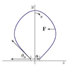
Figure 4: The geometry of our 2D exercise. The contour length of the DNA in the loop is $L$. The size of the protein complex is represented by $a$; its geometry is summarized by the parameter $\theta_{a}$. $a$ and $\theta_{a}$ determine the boundary conditions for the boundary value problem for the geometry of the loop. The element at arclength $s$ from the center exerts a force $\mathbf{F}$ on the element at $s+{\mathrm{d}}s$. Due to the assumed symmetry, $\mathbf{F}$ points along the negative $z$-axis as shown. $\mathbf{F}$ is also the sideways force exerted on the ends of the rod by the protein complex.

As a warmup problem, we consider the analogous elasticity problem in two dimensions. That is, we find the profile $z(s)$ and $y(s)$ of a planar elastic loop (Fig. 4) where $s$ denotes the arc-length along the loop with the origin $s=0$ placed midway along the contour. Our equations will be simple because twist elasticity plays no role in two dimensions.

The boundary value problem for the loop can be stated as

$$K_{\rm bend}\theta^{\prime\prime}+F\sin\theta=0,\qquad\theta(0)=0,\quad\theta({\textstyle\frac{L}{2}})=\pi+\theta_{a},$$ (7)

where $K_{\rm bend}$ is the bending modulus of the elastic rod, $\theta(s)$ is the angle from the positive $z$-axis to the tangent and $\mathbf{F}$ is an unknown force acting along the $z$-axis and exerted by the end-clamp on the rod. Primes denote differentiation with respect to the arclength $s$.

The solution to the second order differential equation above is well known niz99a and can be written as

$$\theta(s)=2\mathrm{am}(\frac{s}{\lambda k}|k),$$ (8)

where $\mathrm{am}(x|k)$ is the elliptic function of the first kind with modulus $k$. $\lambda=\sqrt{\frac{K_{\rm bend}}{F}}$ and $k$ are independent parameters, to be determined from the boundary data. Thus

$$\cos\theta(s)=\frac{{\mathrm{d}}z}{{\mathrm{d}}s} = 1-2\mathrm{sn}^{2}(\frac{s}{\lambda k}|k),$$ (9)

$$\sin\theta(s)=\frac{{\mathrm{d}}y}{{\mathrm{d}}s} = 2\mathrm{sn}(\frac{s}{\lambda k}|k)\mathrm{cn}(\frac{s}{\lambda k}|k).$$ (10)

We can integrate these equations and obtain the following solution for $z(s)$ and $y(s)$, which are the coordinates of the material point denoted by $s$ on the rod:

$$z(s) = s-2\int_{0}^{s}\mathrm{sn}^{2}(\frac{\alpha}{\lambda k}|k){\mathrm{d}}\alpha,$$ (11)

$$y(s) = \int_{0}^{s}2\mathrm{sn}(\frac{\alpha}{\lambda k}|k)\mathrm{cn}(\frac{\alpha}{\lambda k}|k){\mathrm{d}}\alpha=\frac{2\lambda}{k}(1-\mathrm{dn}(\frac{s}{\lambda k}|k)).$$ (12)

Fig. 4 shows a typical solution from this family.

The two constants $\lambda$ and $k$ can be determined in terms of the given $a$ and $\theta_{a}$ by imposing the boundary conditions, leading to the following two equations:

$$\pi+\theta_{a} = \theta(\frac{L}{2})=2\mathrm{am}(\frac{L}{2\lambda k}|k),$$ (13)

$$\frac{a}{2} = \frac{L}{2}-2\int_{0}^{L/2}\mathrm{sn}^{2}(\frac{\alpha}{\lambda k}|k){\mathrm{d}}\alpha.$$ (14)

We denote $y_{p}\equiv\frac{L}{2\lambda k}$ and eliminate $\lambda$ in favor of $y_{p}$, obtaining

$$\pi+\theta_{a} = 2\mathrm{am}(y_{p}|k),$$ (15)

$$y_{p}(1-\frac{a}{L}) = 2\int_{0}^{y_{p}}\mathrm{sn}^{2}(\beta|k){\mathrm{d}}\beta=\frac{2}{k^{2}}(y_{p}-E(y_{p}|k)),$$ (16)

where $E(y_{p}|k)=\int_{0}^{y_{p}}\mathrm{dn}^{2}(x|k){\mathrm{d}}x$ is the incomplete elliptic integral of the second kind with modulus $k$. Once we solve numerically for $y_{p}$ and $k$ from these equations we can obtain the unknown force $F$ as

$$F=\frac{K_{\rm bend}}{\lambda^{2}}=\frac{4K_{\rm bend}y_{p}^{2}k^{2}}{L^{2}}.$$ (17)

Also, the bending moment $M$ applied by the protein at $s=\frac{L}{2}$ is given by

$$M=K_{\rm bend}\theta^{\prime}({\textstyle\frac{L}{2}})=4K_{\rm bend}\frac{y_{p}}{L}\sqrt{1-k^{2}\cos^{2}\frac{\theta_{a}}{2}}.$$ (18)

Finally we calculate the elastic energy stored in the loop.

$${\cal E}_{\rm elas}[\theta(s)] = \int_{-L/2}^{L/2}\Big{(}\frac{K_{\rm bend}}{2}\theta^{\prime 2}(s)-F\cos\theta(s)\Big{)}{\mathrm{d}}s$$ (19)

$$= F\int_{-L/2}^{L/2}\Big{(}\frac{2}{k^{2}}\mathrm{dn}^{2}(\frac{s}{\lambda k}|k)+2\mathrm{sn}^{2}(\frac{s}{\lambda k}|k)-1\Big{)}{\mathrm{d}}s$$

$$= F\int_{-L/2}^{L/2}\Big{(}\frac{2}{k^{2}}-1\Big{)}=FL(\frac{2}{k^{2}}-1).$$

Similar formulas have appeared in earlier work (e.g. cole95a ).

It is well known that the equations describing the shape of a bent rod are similar to the equations of motion of a pendulum and that this analogy can be utilized to obtain rod shapes corresponding to different regimes niz99a . In the above we looked at the solution corresponding to the revolving orbits of the pendulum. We can also have solutions corresponding to oscillating orbits of the pendulum. In that case the solution is given by

$$\cos\theta(s)=1-2k^{2}\mathrm{sn}^{2}(\frac{s}{\lambda}|k).$$ (20)

Corresponding to this solution we find that

$$F=\frac{4K_{\rm bend}y_{p}^{2}}{L^{2}},\qquad M=\frac{4y_{p}K_{\rm bend}}{L}\sqrt{k^{2}-\cos^{2}\frac{\theta_{a}}{2}},\qquad{\cal E}_{\rm elas}[\theta(s)]=FL(2k^{2}-1).$$ (21)

IV.B Elasticity theory: 3D calculation

IV.B.1 $\star$-loop

The $\star$-loop is by definition a planar, untwisted solution of the elastic equilibrium problem with given separation and tangent vectors at the ends. As such its centerline coincides with the 2D solution found in Sect. IV.A above. Its physical frame has $\hat{\mathbf{e}}_{3}$ and $\hat{\mathbf{e}}_{1}$ always in the $yz$ plane, and $\hat{\mathbf{e}}_{2}$ along $\hat{\mathbf{x}}$.

IV.B.2 Rod equilibrium

We now repeat our exercise for a uniform, inextensible, isotropic elastic rod with twist stiffness, not necessarily confined to a plane. We again idealize the protein complex forming the loop as a rigid object attaching to two specified points (representing specific binding sites) on the rod. We assume that the length of the vector connecting one binding site to the other is given, and we call it $a=|\mathbf{a}|$. The orientation of the physical frame attached at one site relative to the one attached at the other site, as well as the orientation of $\mathbf{a}$ relative to either of those frames, are also assumed to be given. The derivatives of the untwisted frame vectors $\{\hat{\mathbf{d}}_{i}(s)\}$ as the arc-length $s$ changes contain information about the local curvature and torsion of the rod:

$$\hat{\mathbf{d}}_{i}^{\prime}=\mbox{\boldmath$\kappa$}\times\hat{\mathbf{d}}_{i},\qquad\mbox{for}\quad i=1,2,3.$$ (22)

We define $\kappa_{1,2,3}$ as the components of the curvature vector $\mbox{\boldmath$\kappa$}(s)$ expanded in the frame $\{\hat{\mathbf{d}}_{i}\}$.

The moment (or torque) $\mathbf{M}(s)$ at any point on the rod is assumed to have the Bernoulli–Euler form

$$\mathbf{M}=K_{\rm bend}\kappa_{1}\hat{\mathbf{d}}_{1}+K_{\rm bend}\kappa_{2}\hat{\mathbf{d}}_{2}+K_{\rm tw}\kappa_{3}\hat{\mathbf{d}}_{3},$$ (23)

where $K_{\rm bend}$ and $K_{\rm tw}$ are the bending and twisting moduli of the elastic rod. Equivalently we can specify the persistence lengths $\xi_{\rm b}=K_{\rm bend}/{k_{\rm B}T}$ and $\xi_{\rm tw}=K_{\rm tw}/{k_{\rm B}T}$, where ${k_{\rm B}T}$ is the thermal energy scale. The equilibrium equation for the rod is then simply given by force balance, $\mathbf{F}^{\prime}=\mathbf{0}$, and by torque balance:

$$\mathbf{M}^{\prime}+\hat{\mathbf{d}}_{3}\times\mathbf{F}=\mathbf{0}.$$ (24)

As in Fig. 4, $\mathbf{F}(s)$ is the force each element exerts on the next; it is also the force applied by the protein on the DNA.

Following Nizette and Goriely niz99a , we will assume that the laboratory coordinate frame is chosen in such a way that the constant internal force $\mathbf{F}$ is aligned with the laboratory $z$-axis: $\mathbf{F}=F\hat{\mathbf{z}}$. We write the position vector $\mathbf{P}(s)$ of any point on the loop as $[X(s),Y(s),Z(s)]$ or in cylindrical coordinates as $[R(s),\Phi(s),Z(s)]$:

$$\mathbf{P}(s) = X(s)\hat{\mathbf{x}}+Y(s)\hat{\mathbf{y}}+Z(s)\hat{\mathbf{z}}$$ (25)

$$= R(s)\cos\Phi(s)\hat{\mathbf{x}}+R(s)\sin\Phi(s)\hat{\mathbf{y}}+Z(s)\hat{\mathbf{z}}.$$

Because we assume that our protein complex obeys the symmetric coupler condition (Sect. II.B.3), we will be interested in loops that are also symmetric in a way that generalizes Fig. 4. Specifically, we will find suitable equilibrium solutions satisfying our boundary conditions, which also obey

$$X(s)=-X(-s),\qquad Y(s)=Y(-s),\qquad Z(s)=-Z(-s).$$ (26)

Eqs. 26 reduce to our planar form when $X(s)\equiv 0$. It may appear to treat the $X$ and $Y$ directions asymmetrically, but what is meant is that the solutions of interest can be brought to this form by translation and rotation about $\hat{\mathbf{z}}$. Thus for example, if the loop is planar then we agree to place it in the $yz$-plane, with the center point $s=0$ at the origin. Eqs. 26 suggest that $\Phi(s)$ will take the form $\Phi(s)=\frac{\pi}{2}-\alpha(s)$ with $\alpha(-s)=-\alpha(s)$, and indeed our solutions will have this property.

IV.B.3 Boundary conditions

We are now in a position to formulate the boundary condition describing the relative position of the ends of the loop. Our first condition again imposes a separation of length $a$:

$$\|\mathbf{P}({\textstyle\frac{L}{2}})-\mathbf{P}(-{\textstyle\frac{L}{2}})\|^{2}=a^{2},$$ (27)

where again $L$ is the loop contour length. Taking account of the symmetry of the loop, this statement amounts to

$$R^{2}({\textstyle\frac{L}{2}})\cos^{2}\Phi({\textstyle\frac{L}{2}})+Z^{2}({\textstyle\frac{L}{2}})=\frac{a^{2}}{4}.$$ (28)

Notice that our choice of loop orientation implies that the end-to-end vector of the loop $\mathbf{a}$ lies in the $xz$-plane, though not in general along the $z$-axis as in Fig. 4.

The tangent vector at any point on the rod is given by $\hat{\mathbf{t}}(s)=\frac{\mathbf{P}^{\prime}(s)}{\|\mathbf{P}^{\prime}(s)\|}$. Explicitly,

$$\mathbf{P}^{\prime}(s)=(R^{\prime}(s)\cos\Phi(s)-R(s)\Phi^{\prime}(s)\sin\Phi(s))\hat{\mathbf{x}}+(R^{\prime}(s)\sin\Phi(s)+R(s)\Phi^{\prime}(s)\cos\Phi(s))\hat{\mathbf{y}}+Z^{\prime}(s)\hat{\mathbf{z}}$$ (29)

which can be rewritten as

$$\hat{\mathbf{t}}(s)=\mathbf{P}^{\prime}(s)=T(s)\cos\phi(s)\hat{\mathbf{x}}+T(s)\sin\phi(s)\hat{\mathbf{y}}+\cos\theta(s)\hat{\mathbf{z}}$$ (30)

where we define $\theta(s)$, $\phi(s)$ and $T(s)$ through

$$\cos\theta(s) = Z^{\prime}(s),$$ (31)

$$\tan\phi(s) = \tan\left(\Phi(s)+\tan^{-1}\frac{R(s)\Phi^{\prime}(s)}{R^{\prime}(s)}\right),$$ (32)

$$T^{2}(s) = R^{\prime 2}(s)+R^{2}(s)\Phi^{\prime 2}(s)=1-Z^{\prime 2}(s).$$ (33)

The last equation reflects the inextensibility of the rod.

Our planar coupler requires that the vectors $\mathbf{a}$, $\mathbf{P}^{\prime}(-\frac{L}{2})$ and $\mathbf{P}^{\prime}(\frac{L}{2})$ all lie in a common plane, even if the full loop is not planar. Accordingly, we will seek solutions satisfying a second boundary condition:

$$\mathbf{a}\cdot(\mathbf{P}^{\prime}(-{\textstyle\frac{L}{2}})\times\mathbf{P}^{\prime}({\textstyle\frac{L}{2}}))=0.$$ (34)

Using the assumed symmetry of the shape of the loop, we see that this boundary condition can be satisfied if either

$$\frac{a_{x}}{a_{z}}=\frac{R(\frac{L}{2})\cos\Phi(\frac{L}{2})}{Z(\frac{L}{2})}=\frac{R^{\prime}(\frac{L}{2})\cos\Phi(\frac{L}{2})-R(\frac{L}{2})\Phi^{\prime}(\frac{L}{2})\sin\Phi(\frac{L}{2})}{Z^{\prime}(\frac{L}{2})},$$ (35)

or

$$R^{\prime}({\textstyle\frac{L}{2}})\sin\Phi({\textstyle\frac{L}{2}})+R({\textstyle\frac{L}{2}})\Phi^{\prime}({\textstyle\frac{L}{2}})\cos\Phi({\textstyle\frac{L}{2}})=0.$$ (36)

Substituting Eq. 36 into Eq. 32 shows that the second of these conditions would imply $\phi(\pm\frac{L}{2})=0$. This in turn would imply that the end tangents $\mathbf{P}^{\prime}(\pm\frac{L}{2})$ are parallel and lie on the $xz$-plane. This violates the assumed geometry of the coupler depicted in Fig. 2: The end tangents need not be parallel. So in this section we pursue only the condition represented by Eq. 35, which allows for loops with the desired coupler geometry.

The third boundary condition that we need to satisfy involves the angle at which the DNA exits the protein complex. Generalizing Eq. 7, we will require that

$$\mathbf{a}\cdot\mathbf{P}^{\prime}({\textstyle\frac{L}{2}})=a\cos\theta_{a}.$$ (37)

Together Eqs. 27, 35 and 37 can be recast as the boundary conditions

$$\frac{Z^{\prime}(\frac{L}{2})}{Z(\frac{L}{2})} = \frac{2\cos\theta_{a}}{a},$$ (38)

$$R^{2}({\textstyle\frac{L}{2}})\cos^{2}\Phi({\textstyle\frac{L}{2}})+Z^{2}({\textstyle\frac{L}{2}}) = \frac{a^{2}}{4},$$ (39)

$$\frac{R^{\prime}(\frac{L}{2})}{R(\frac{L}{2})}-\Phi^{\prime}({\textstyle\frac{L}{2}})\tan\Phi({\textstyle\frac{L}{2}}) = \frac{2\cos\theta_{a}}{a}.$$ (40)

We will solve these equations starting from the most general solution to the differential equations for the equilibrium of a bent and twisted rod. The solution yields analytical expressions for $R(s)$, $Z(s)$ and $\Phi(s)$, which will be substituted in the above to obtain algebraic equations. Nizette and Goriely niz99a give the solution in terms of four parameters $\zeta_{1,2,3}$ and $\lambda$ as

$$Z(s) = \zeta_{3}s-\lambda(\zeta_{3}-\zeta_{1})E(\frac{s}{\lambda}|k),$$ (41)

$$R^{2}(s) = 2\lambda^{2}(\tilde{h}-Z^{\prime}(s)),$$ (42)

$$\Phi(s) = \frac{\lambda}{2K_{\rm bend}}\Big{(}M_{z}\frac{s}{\lambda}+\frac{M_{3}-M_{z}\tilde{h}}{\tilde{h}-\zeta_{1}}\Pi(\frac{s}{\lambda}|\tilde{n},k)\Big{)}-\frac{\pi}{2},$$ (43)

where $\Pi$ is the elliptic integral of the third kind and

$$M_{3} = \frac{K_{\rm bend}}{\sqrt{2}\lambda}\left(\sqrt{(1+\zeta_{1})(1+\zeta_{2})(\zeta_{3}+1)}+\sqrt{(1-\zeta_{1})(1-\zeta_{2})(\zeta_{3}-1)}\right),$$ (44)

$$M_{z} = \frac{K_{\rm bend}}{\sqrt{2}\lambda}\left(\sqrt{(1+\zeta_{1})(1+\zeta_{2})(\zeta_{3}+1)}-\sqrt{(1-\zeta_{1})(1-\zeta_{2})(\zeta_{3}-1)}\right),$$ (45)

$$\tilde{h} = \frac{1}{2}\Big{[}\zeta_{1}+\zeta_{2}+\zeta_{3}-\zeta_{1}\zeta_{2}\zeta_{3}+\sqrt{(1-\zeta_{1}^{2})(1-\zeta_{2}^{2})(\zeta_{3}^{2}-1)}\Big{]},$$ (46)

$$\tilde{n} = \frac{\zeta_{2}-\zeta_{1}}{\tilde{h}-\zeta_{1}},\qquad k^{2}=\frac{\zeta_{2}-\zeta_{1}}{\zeta_{3}-\zeta_{1}}\qquad n=\frac{\zeta_{2}-\zeta_{1}}{h-\zeta_{1}}.$$ (47)

The quantities $M_{3}$ and $M_{z}$ turn out to be the components of the moment vector along $\hat{\mathbf{d}}_{3}$ and $\hat{\mathbf{z}}$, respectively niz99a .

We must now fix the parameters $\zeta_{1,2,3}$ and $\lambda$ by imposing boundary conditions. In addition to Eqs. 38–40, we also need an expression for how the frames at each end of the rod are oriented with respect to each other. To formulate such an expression, note that for any choice of $a$ and $\theta_{a}$ there will be one non-selfintersecting loop solution with zero excess twist — the $\star$-loop. Taking this as a reference configuration, any other equilibrium solution with the same $a$ and $\theta_{a}$ and the same initial $\hat{\mathbf{d}}_{1}(-\frac{L}{2})=\hat{\mathbf{d}}_{1,{\rm ref}}(-\frac{L}{2})$ will have a final orientation $\hat{\mathbf{d}}_{1}(+\frac{L}{2})$ differing from $\hat{\mathbf{d}}_{1,{\rm ref}}(+\frac{L}{2})$ by a rotation about $\hat{\mathbf{t}}(+\frac{L}{2})$. We need to find the corresponding rotation angle $\psi$, then impose the condition Eq. 5.

The angle $\psi$, divided by $2\pi$, may be regarded as a linking number difference, generalized to the case of open curves. To evaluate it, we need a generalization of the Fuller–White–Calugareanu relation $\Delta\mathrm{Lk}=\Delta\mathrm{Tw}+\Delta\mathrm{Wr}$ for open curves. We start with the $\star$-loop, with its untwisted frame. Next we construct a plane, untwisted, circular arc $C$, attached to the two ends of the $\star$-loop to form a closed, smooth, framed curve. Completing the $\star$-loop in this way gives a closed loop with $\mathrm{Tw}=\mathrm{Wr}=0$. Also, the tangents at the ends of $C$ match the tangents at the ends of any of the family of loops we are studying.

Completing any other loop in our family with the same $C$ gives a discontinuity in the axial orientation at one of the attachment points. Hence the formula for linking number will not give an integer; instead, $2\pi\mathrm{Lk}$ is the desired formula for $\psi$. Setting it equal to one of the desired values (Eq. 5) gives our fourth boundary condition.

In summary, our fourth boundary condition is $\psi=(L-L_{0})\omega_{0}+2\pi n$ for an integer $n$, where kami02a

$$\psi=2\pi\mathrm{Lk} = 2\pi(\mathrm{Tw}+\mathrm{Wr})$$ (48)

$$= \int_{-\frac{L}{2}}^{\frac{L}{2}}\kappa_{3}{\mathrm{d}}s+\frac{1}{2}\oint\oint\hat{\mathbf{t}}(s)\cdot\hat{\mathbf{t}}(s^{\prime})\times\frac{\mathbf{P}(s)-\mathbf{P}(s^{\prime})}{\|\mathbf{P}(s)-\mathbf{P}(s^{\prime})\|^{3}}\,{\mathrm{d}}s\,{\mathrm{d}}s^{\prime}.$$

Here $\oint\ldots{\mathrm{d}}s$ refers to a line integral over the closed loop consisting of the arc $C$ plus the open loop under study.

IV.B.4 Solution strategy

There are four parameters in the above equations: $\zeta_{1}$, $\zeta_{2}$, $\zeta_{3}$ and $\lambda$. As in Sect. IV.A, we must find values for these parameters by imposing the boundary conditions. These four parameters can be determined by enforcing the boundary conditions (Eqs. 27, 35, 37, and 48). This leads to a set of equations that must be solved numerically, using Newton’s method. Our initial guess for $\zeta_{1}$, $\zeta_{2}$, $\zeta_{3}$ and $\lambda$ for given boundary data corresponds to the values of these parameters for a planar loop. For example, we know how to solve for $k$ and $\lambda$ for a planar loop (for which $\psi=0$) of length $L$, end-separation $a$ and end-angle $\theta_{a}$. For a three dimensional loop with similar data (but $\psi\neq 0$) we initialize Newton’s method with the guess $\zeta_{1}=-1$, $\zeta_{2}=2k^{2}-1$, $\zeta_{3}=1$. We then make a small increment in $\psi$ and solve a system of four algebraic equations to obtain the nearby values of $\zeta_{1}$, $\zeta_{2}$, $\zeta_{3}$ and $\lambda$ that give this value of $\psi$. We continue this incremental process until we have achieved one of the values of $\psi_{n}$ dictated by the contour length $L$ between the repressor binding sites (Eq. 5). This numerical procedure corresponds physically to holding a rod into a planar loop and subsequently rotating one end, continuously changing the shape of the loop. Once we have computed this solution, the elastic energy stored in the DNA is evaluated using the following expression (see niz99a ):

$${\cal E}_{n}=\frac{FL}{2}\Big{[}\zeta_{1}+\zeta_{2}+\zeta_{3}-\zeta_{1}\zeta_{2}\zeta_{3}-\sqrt{(1-\zeta_{1}^{2})(1-\zeta_{2}^{2})(\zeta_{3}^{2}-1)}\Big{]}+\frac{{M_{3}}^{2}L}{2K_{\rm tw}}.$$ (49)

Then we continue the incremental search both forward and backward in $\psi$ looking for other topoisomers.

V Results

Our goal is to capture certain broad features of the looping free energy change as obtained from experiments in the analysis of Refs. saiz05a ; garc?a (Fig. 1b). Beyond the gross structure, there is a shallow minimum in the looping free energy change, in the 70–80bp range. Keeping in mind that the horizontal axis of the graph differs from our $L$ by 21 bp, this minimum corresponds to $L\approx 50$–60 bp. In contrast, for loops formed in cyclization reactions clou05b the minimum in free energy change occurs at about 500bp shim84a . We will see that our elastic rod model, incorporating supercoiling effects and a highly simplified form of the geometry of the repressor–DNA complex, does reproduce some qualitative features in the length dependence of the free energy change. To do this, we now apply the methods of analysis outlined in the previous sections.

Sect. II described the idealizations we have made to keep the role of external torsional stress as clear as possible. These idealizations limit our ability to make quantitative predictions for specific systems, but nevertheless we will apply our method using parameters partially inspired by the structure of the lac repressor complex. Thus, we estimate the distance between the two ends of the DNA to be $a\approx 4.0\,$nm. We estimate $M_{\rm ext}=-1.0\,{k_{\rm B}T}$ (see Sect. II.A.2), and take effective values for the elastic constants from experiments on the cyclization of short DNA: $\xi_{\rm b}=50\,$nm, $\xi_{\rm tw}=18\,$nm clou05b . Finally, we make initial guesses $\theta_{a}=71^{\circ}$ and $L_{0}=0$ for the unknown parameters.

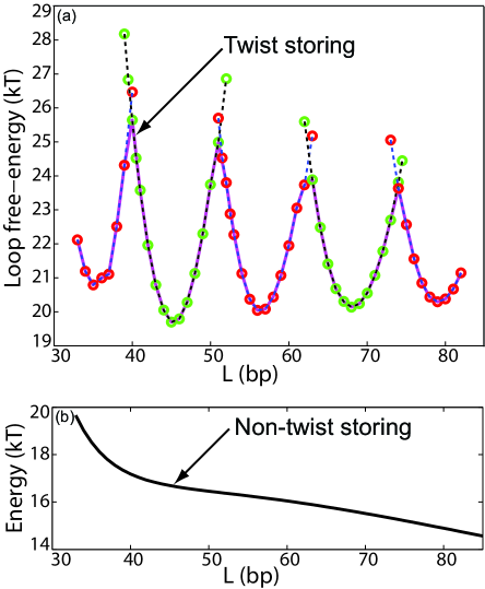
Figure 5: a. The elastic energy of DNA loops as calculated from an elastic rod model of DNA. We have assumed $\theta_{a}=71^{\circ}$ and $a=4.0$nm with $\xi_{p}=50$nm, $\xi_{t}=18$nm and $M_{\rm ext}=-1.0{k_{\rm B}T}$. The graph shows the quantity defined in Eq. 6, plus an arbitrary linear function of $L$, because such a function was dropped in our derivation of Eq. 6. The exchange of stability between various topoisomers at the peaks of the modulations (40,52,63,74bp) has been emphasized by plotting the energy of the two competing topoisomers with different symbols (circles and stars). The continuous line connects the lowest energy topoisomers at each value of the length $L$ of the loop. b. The black curve plots the elastic energy of a planar loop without any twist, as calculated using Eq. 19. This curve would be appropriate for looping with nicked DNA.

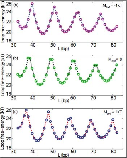
Figure 6: Predicting the effect of changing the sign and magnitude of $M_{\rm ext}$. Again we took $\theta_{a}=71^{\circ}$ and $a=4.0$nm with $\xi_{b}=50$nm, $\xi_{tw}=18$nm and plotted the energy for three values of $M_{\rm ext}$. All three panels have the same, arbitrary, linear function of $L$ added to the looping free energy change. The sign of the assumed torque $M_{\rm ext}$ in panel (c) is the opposite of that in panel (a). The minima and maxima in panel (c) are shifted by about 4 bp as compared to those in panel (a).

Fig. 5 shows the free energy of loops with $M_{\rm ext}=-1.0{k_{\rm B}T}$. This result shows that a simple elastic rod model of the DNA is able to capture the general trend in the modulations of the free energy. The amplitude of the modulations (about $4{k_{\rm B}T}$) is correctly reproduced and the maxima of the modulations are sharp, as found from experimental data by Saiz et al. saiz05a . The curve also shows a dip in free energy at about 45 bp, fairly close to the dip in the experimental data. No such dip is seen in the free energy of looping for nicked (non-twist storing) DNA, so its appearance is influenced by the external torque due to supercoiling.

Fig. 6 shows the looping free energy change as a function of length for the three values $M_{\rm ext}=-1,0,$ and $+1{k_{\rm B}T}$, illustrating our point that the exchanges of stability that determine the dominant topoisomer at a given value of $L$ depend on the magnitude and sign of the external torsional stress. This is easily seen by comparing panels (a) and (c) of Fig. 6 which show that changing the sign of $M_{\rm ext}$ shifts the maxima of the modulations by about 4 bp. The sign of $M_{\rm ext}$ can in principle be controlled in an in vitro experiment, such as a magnetic bead assay (employed in Lia et al. lia03a ). As a result the preference for a particular topoisomer of a loop will change and this will result in an altered dependence of the looping free energy on the contour length. Fig. 6 summarizes how this dependence will be altered for zero torque and a positive torque. Fig. 6 has been constructed for the geometry of the lac repressor but the conclusion that the magnitude and sign of the external torque $M_{\rm ext}$ controls the locations of the minima and maxima of the modulations in the free energy of loop formation remains valid for any other DNA looping protein as well.

VI Discussion

We have shown in this paper that an elastic rod model of DNA can explain certain the features observed in the length dependence of in vivo DNA looping free energy, if we account for the size and shape of the repressor–DNA complex, and for the external torsional stress from supercoiling in the bacterial chromosome. These features have not been adequately examined in the theoretical literature, although they are critical in determining the function of the repressor–DNA complex. We have also obtained predictions that could elucidate the mechanics of protein–DNA interactions, and we hope that they will inspire future experiments. One can adjust $M_{\rm ext}$ in vivo by studying bacteria with varying levels of supercoiling density, for example by disabling the topoisomerases that normally maintain the genome under torsional stress (volobook ). Or the present theory can be generalized to incorporate the effects of stretching force; then a magnetic bead assay could be used to test our prediction that the locations of the minima and maxima in the modulations of the free energy of loop formation can be controlled by the applied external torque. An important limitation of our theory, as presently stated, is that it does not address entropic effects and therefore is applicable only for short contour lengths of DNA.However, the efficient numerical approach developed in this paper remains applicable for longer contour lengths as well and could be used in conjunction with Monte Carlo methods or Molecular Dynamics to explore the effects of entropy on the mechanics of protein DNA interactions.

Appendix A Summary of notation

• $K_{\rm bend}$, $K_{\rm tw}$ are the bend and torsional elastic constants of DNA; the corresponding persistence lengths are $\xi_{\rm b}$ and $\xi_{\rm tw}$.
  $\omega_{0}$ is the natural twist rate of DNA, about $2\pi$ radians per 11bp. $L_{\rm helix}$ is the helix pitch of DNA, about 11bp.

• $s_{\rm i}$, $s_{\rm f}$ are the arclength positions at which the DNA exits its binding sites and enters the loop interior; $\tilde{s}_{\rm i}$, $\tilde{s}_{\rm f}$ are the corresponding positions where the DNA enters the exterior region.
  $L=s_{\rm i}-s_{\rm f}$ is the spacing between exit points; $L_{0}$ is a special value of this spacing for which the coupler admits a planar, untwisted loop.

• $\{\hat{\mathbf{e}}_{i}(s),i=1,2,3\}$ denote the physical orthonormal frame attached to the DNA at arclength position $s$; $\{\hat{\mathbf{d}}_{i}(s)\}$ is the corresponding untwisted frame.
  $\kappa_{1,2,3}(s)$ denote components of the curvature vector at location $s$, measured in the untwisted frame.
  $\hat{\mathbf{t}}=\hat{\mathbf{e}}_{3}=\hat{\mathbf{d}}_{3}$ is the tangent vector to the DNA centerline, as a function of arclength position along the DNA.

• The “coupler” refers to a geometrical representation of a regulatory protein complex, imposing a fixed relation between the spatial locations and physical orientations of two points on the DNA. It is independent of the spacing $L$. A “physical loop configuration” is one obeying the boundary conditions imposed by the coupler.
  The “$\star$-coupler” is a fictitious, modified coupler differing from the physical one by an $L$-dependent axial rotation of one of the DNA strands relative to the other. Quantities associated to it are denoted by a subscript $\star$. The “$\star$-loop configuration” is the loop of minimal elastic energy obeying the boundary conditions imposed by the $\star$-coupler.
  $\mathbf{a}$ is the spatial separation between DNA detachment points; $a$ denotes its length.
  $\theta_{a}$ is the exit angle characterizing the regulatory protein complex.
  $\beta\qquad$ twist angle of the DNA–protein complex, set equal to zero in this paper

• $M_{\rm ext}\qquad$ torsional stress outside the looping region, same units as energy; $M_{1,2,3}(s)$ are the components of the moment (torque) vector inside the loop at arclength position $s$, expressed in the untwisted frame. Note that $M_{\rm ext}\not=M_{3}$ in general.

• ${\cal E}_{\star}$ denotes the elastic energy of the lowest-energy $\star$-loop configuration; ${\cal E}$ denotes the elastic energy of a physical looped state.
  $n$ indexes which of the possible physical loop states is under discussion; ${\cal U}$ is the unlooped state.
  $\psi_{n}$ is the axial rotation angle by which physical loop $n$ differs from the $\star$-loop.

• $G_{\rm un}(L_{\mathrm{tot}},\sigma)\qquad$ denotes the free energy of an unlooped circular DNA of length $L_{\mathrm{tot}}$ with fractional excess linking number $\sigma$; $\mu(\sigma)$ is the corresponding free energy per unit length.

• $\mathrm{am},\mathrm{sn},\mathrm{cn}$ are the usual elliptic functions. $k$ is the modulus of an elliptic function. $E(y|k)$ is the incomplete elliptic integral of the second kind; $\Pi(y|n,k)$ is the elliptic function of the third kind.

• $\zeta_{1,2,3}$ are parameters entering the general elastic equilibrium solution in 3D.
  $R(s),\Phi(s),Z(s)$ are cylindrical coordinates for the position of the rod at arclength position $s$.
  $\theta(s),\phi(s)$ are spherical polar coordinates for the unit tangent vector to the rod at position $s$.

References

- (1) T. Dunn, S. Hahn, S. Ogden, and R. Schleif, Proc. Natl. Acad. Sci. USA 81, 5017 (1984).
- (2) S. Adhya, Annual Review of Genetics 23, 227 (1989).
- (3) R. Schleif, Annual Review of Biochemistry 61, 199 (1992).
- (4) S. E. Halford, A. J. Welsh, and M. D. Szczelkun, Annual Review of Biophysics and Biomolecular Structure 33, 1 (2004).
- (5) A. Hochschild and M. Ptashne, Cell 44, 925 (1986).
- (6) H. Krämer et al., Embo Journal 6, 1481 (1987).
- (7) G. R. Bellomy, M. C. Mossing, and M. T. Record, Biochemistry 27, 3900 (1988).
- (8) J. Müller, S. Oehler, and B. Müller-Hill, Journal of Molecular Biology 257, 21 (1996).
- (9) N. A. Becker, J. D. Kahn, and L. J. Maher, Journal of Molecular Biology 349, 716 (2005), erratum ibid 353 (4): 924-926 2005.
- (10) L. Saiz, J. M. Rubi, and J. M. G. Vilar, Proceedings of the National Academy of Sciences of the United States of America 102, 17642 (2005).
- (11) H. G. Garcia, L. Bintu, P. A. Wiggins, J. Kondev and R. Phillips (unpublished 2006).
- (12) M. C. Mossing and M. T. Record, Science 233, 889 (1986).
- (13) M. Lewis et al., Science 271, 1247 (1996).
- (14) A. Balaeff, L. Mahadevan, and K. Schulten, Physical Review Letters 83, 4900 (1999).
- (15) L. Finzi and J. Gelles, Science 68, 378 (1995).
- (16) G. Lia et al., Proc. Natl. Acad. Sci. USA 100, 11373 (2003).
- (17) C. E. Bell, J. Barry, K. S. Matthews, and M. Lewis, Journal of Molecular Biology 313, 99 (2001).
- (18) C. E. Bell and M. Lewis, Journal of Molecular Biology 312, 921 (2001).
- (19) L. Bintu et al., Current Opinion in Genetics & Development 15, 116 (2005).
- (20) L. L. Saiz and J. M. G. Vilar, preprint arXiv:q-bio.BM/0602012 (unpublished).
- (21) K. V. Klenin, M. D. Frank-Kamenetskii, and J. Langowski, Biophysical Journal 68, 81 (1995).
- (22) A. Vologodskii and N. R. Cozzarelli, Biophysical Journal 70, 2548 (1996).
- (23) A. V. Vologodskii, Topology and physics of circular DNA (CRC Press, Boca Raton, 1992).
- (24) M. Geanacopoulos, G. Vasmatzis, V. B. Zhurkin, and S. Adhya, Nature Structural Biology 8, 432 (2001).
- (25) C. E. Bell, P. Frescura, A. Hochschild, and M. Lewis, Cell 101, 801 (2000).
- (26) I. Tobias, D. Swigon, and B. D. Coleman, Physical Review E 61, 747 (2000).
- (27) O. V. Tsodikov et al., Journal of Molecular Biology 294, 639 (1999).
- (28) A. Balaeff, C. R. Koudella, L. Mahadevan, and K. Schulten, Philosophical Transactions of the Royal Society of London Series A—Mathematical Physical and Engineering Sciences 362, 1355 (2004).
- (29) A. Balaeff, L. Mahadevan, and K. Schulten, Structure (Camb) 12, 123 (2004).
- (30) N. Douarche and S. Cocco, Physical Review E 72, 061902 (2005).
- (31) A. Balaeff, L. Mahadevan, and K. Schulten, Physical Review E 73, 031919 (2006).
- (32) I. Tobias, B. D. Coleman, and W. K. Olson, Journal of Chemical Physics 101, 10990 (1994).
- (33) B. D. Coleman, I. Tobias, and D. Swigon, Journal of Chemical Physics 103, 9101 (1995).
- (34) D. Swigon, B. D. Coleman, and W. K. Olson, Proceedings of the National Academy of Sciences of the United States of America 103, 9879 (2006).
- (35) J. Shimada and H. Yamakawa, Macromolecules 17, 689 (1984).
- (36) Y. L. Zhang and D. M. Crothers, Biophysical Journal 84, 136 (2003).
- (37) A. J. Spakowitz, Europhys. Lett. 73, 684 (2006).
- (38) Y. Zhang, A. E. McEwen, D. M. Crothers, and S. D. Levene, Biophysical Journal 90, 1903 (2006).
- (39) Y. Zhang, A. E. McEwen, D. M. Crothers, and S. D. Levene, (2006), (unpublished).
- (40) E. Villa, A. Balaeff, L. Mahadevan, and K. Schulten, Multiscale Modeling and Simulation 2, 527 (2004).
- (41) E. Villa, A. Balaeff, and K. Schulten, Proceedings of the National Academy of Sciences of the United States of America 102, 6783 (2005).
- (42) J. B. Bliska and N. R. Cozzarelli, Journal of Molecular Biology 194, 205 (1987).
- (43) K. Drlica, Molecular Microbiology 6, 425 (1992).
- (44) J. F. Marko and E. D. Siggia, Phys. Rev. E52, 2912 (1995).
- (45) A. V. Vologodskii et al., Journal of Molecular Biology 227, 1224 (1992).
- (46) P. A. Wiggins and P. C. Nelson, Phys. Rev. E 73, 031906 (2006).
- (47) P. A. Wiggins et al., Nature Nanotechnology (2006), (In press.).
- (48) T. A. Steitz, T. J. Richmond, D. Wise, and D. Engelman, Proceedings of the National Academy of Sciences of the United States of America 71, 593 (1974).
- (49) P. Nelson, Biological Physics: Energy, Information, Life (W. H. Freeman and Co., New York, 2004), section 6.6.4.
- (50) M. Nizette and A. Goriely, Journal of Mathematical Physics 40, 2830 (1999).
- (51) R. D. Kamien, Rev. Mod. Phys. 74, 953 (2002).
- (52) T. E. Cloutier and J. Widom, Proc. Natl. Acad. Sci. USA 102, 3634 (2005).