Estimating degrees of freedom in motor systems

Abstract

Studies of the degrees of freedom or “synergies” in musculoskeletal systems rely critically on algorithms to estimate the “dimension” of kinematic or neural data. Linear algorithms such as principal component analysis (PCA) are used almost exclusively for this purpose. However, biological systems tend to possess nonlinearities and operate at multiple spatial and temporal scales so that the set of reachable system states typically does not lie close to a single linear subspace. We compare the performance of PCA to two alternative nonlinear algorithms (Isomap and our novel pointwise dimension estimation (PD-E )) using synthetic and motion capture data from a robotic arm with known kinematic dimensions, as well as motion capture data from human hands. We find that consideration of the spectral properties of the singular value decomposition in PCA can lead to more accurate dimension estimates than the dominant practice of using a fixed variance capture threshold. We investigate methods for identifying a single integer dimension using PCA and Isomap. In contrast, PD-E provides a range of estimates of fractal dimension. This helps to identify heterogeneous geometric structure of data sets such as unions of manifolds of differing dimensions, to which Isomap is less sensitive. Contrary to common opinion regarding fractal dimension methods, PD-E yielded reasonable results with reasonable amounts of data. We conclude that it is necessary and feasible to complement PCA with other methods that take into consideration the nonlinear properties of biological systems for a more robust estimation of their degrees of freedom.

1 Introduction

The ability to use sensor data to objectively quantify the number of active or controlled skeletal degrees of freedom (DOFs) during natural behavior is central to the study of neural control of musculoskeletal redundancy. A long standing problem in the study of neuromuscular systems is whether and how the nervous system uses the numerous DOFs provided by the neuro-musculo-skeletal system. For example, several studies have sought to determine whether the nervous system couples the mechanical DOFs of the hand to simplify the control of hand shaping for grasp or sign language [1, 2]. Other important problems are the estimation of dimension of the neural controller from electromyographic signals [3] or extracellular neural recordings from the brain [4]. Theories of motor learning also address problems of dimension estimation by proposing that the acquisition of complex tasks progresses by initially “freezing” some skeletal degrees of freedom and gradually releasing them as the nervous systems is able to incorporate them into the motor task [5].

1.1 Algorithmic methods to estimate the dimension of data

This paper discusses algorithmic methods that measure the dimension in state space occupied by observed dynamical behaviours. Our goal is to compare and contrast the performance of today’s mathematically related, but distinct, definitions of dimension and varied approaches to estimating the dimension of a dynamical system from sampled data. We focus on comparing the performance of two established algorithms—principal component analysis (PCA) [6] and Isomap [7]— with a new algorithm that estimates pointwise dimension (PD-E ).

PCA, linear regression and multi-dimensional scaling (MDS) [8] are linear methods that test whether a data set lies close to a linear subspace, in which case the coordinates from this subspace can be used to parameterize the data. However, these methods do not determine whether the data may lie on a lower dimensional set within the subspace. Indeed, a single arm rotating relative to the body in a plane produces a motion capture data set that lies along a circle, The circle is a one dimensional set because it can be parameterized by a single coordinate (e.g., an angle), but the circle does not lie close to a one dimensional linear subspace. Linear methods suggest that two coordinates are most appropriate in this example, where these coordinates describe the plane in which the circular motion takes place. This is an example where linear methods do not suffice in determining the dimension even of a simple geometric object underlying the motion of a simple kinematic system.

Isomap [7], local linear embedding (LLE) [9], and Laplacian or Hessian eigenmaps [10, 11] are methods that have been developed within the setting of machine learning and dimension reduction to find coordinate systems for nonlinear manifolds. They include procedures for discovering the dimension of data sets that lie on smooth Riemannian manifolds. Isomap seeks a set of global coordinates for this manifold via singular value decomposition of a matrix of interpoint distances of the data.

In our application to biomechanics the underlying structure of the biomechanical system governing, say, locomotion or manipulation, may not be representable as motion in a smooth manifold. The structure might instead decompose as the union of submanifolds having different dimension for different phases in the gait cycle (e.g., swing versus double support) or grasp acquisition versus manipulation. We need techniques that can identify the appropriate decomposition and estimate the dimension of the different phases of the task. This paper shows that PD-E aids in the process of exploring this kind of complex geometric structure in data sets.

Pointwise dimension is a quantity assigned to probability densities or measures that are defined on metric spaces. Like Isomap, algorithms for computing pointwise dimension are based upon analysis of the distances between pairs of data points. However, the way in which this information is used is quite different in the two methods. Algorithms for estimating the pointwise dimension of attractors of dynamical systems were developed in the 1980’s and applied to many different empirical data sets. Much of this work used a technique called “delay embedding” to manufacture multidimensional data from a single (one-dimensional) time series. To use delay embedding effectively the time step between successive observations and the number of successive observations to use in the embedding have to balanced to account for the sensitive dependence of solutions to initial conditions, the dimension of the attractor and the independence of observations made at each time step. There was a consenus that prohibitive amounts of data were required by the methods for accurately estimating the pointwise dimension of high dimensional attractors [12]. This paper revisits the numerical estimation of pointwise dimension in the context of motion capture data, where the emphasis is upon estimating the dimension of sets that are already embedded in high-dimensional Euclidean spaces.

1.2 Goal and approach

We compare and assess the ability of PD-E , PCA, and Isomap methods to estimate the dimension of data sets that are representative of motion capture. The methods are applied to synthetic data sets generated from simple geometric objects and from a numerical simulation of a robot arm. As representative examples of empirical data, we study the kinematic DOFs of a robotic arm and the kinematics of the human fingers using motion capture data. The motion capture data consist of the spatial locations of identified markers placed on the surface of the systems as they assume a large set of postures representative of their workspace.

Our results suggest that estimation of pointwise dimension is a promising tool for the analysis of motion capture data, and in particular we estimate bounds on the DOFs involved in hand kinematics. We suggest avenues to expand the mathematical theory underlying our method, and propose additional empirical testing necessary to explore its most effective use.

2 Methods

2.1 Pointwise fractal dimension

Algorithms for estimating the pointwise and correlation dimensions of data sets were developed in the 1980’s within the context of assigning dimensions to attractors of dynamical systems [13, 14, 15]. These algorithms are framed in the setting of measures or probability densities in a metric space, and assume that the data whose dimension is being determined is distributed like independent samples of the measure. They do not make use of the temporal structure of trajectories and can be applied to arbitrary data sets that give discrete approximations to a probability measure $\mu$. In practice, this means that the $\mu$-measure of a set $S$ (we call this the volume of $S$) can be approximated by the proportion of data points that lie in $S$. Methods such as PCA, Isomap, and LLE presume that input data represent samples from a geometric set with the structure of a Riemannian manifold. In contrast, pointwise dimension and the algorithms used to estimate it make sense for sets that are made up of a union of manifolds having different dimension and for large classes of fractal sets supporting a suitable measure. Biological systems are likely candidates for pointwise dimension approaches given that their structure, function and control operate at different spatial and temporal scales and in different modes simultaneously (e.g., skin vs. fat vs. muscle vs. bone motions; reflex vs. voluntary control of movement; etc.).

The pointwise dimension of $x\in S$ is defined by measuring the growth rate of balls of radius $r$ centered at $x$ as a function of $r$. Denoting the balls by $B_{x}(r)$, the dimension $d_{\mu}(x)$ of $\mu$ at $x$ is

$$d_{\mu}(x)=\lim_{r\to 0}\frac{\log(\mu(B_{x}(r))}{\log(r)}.$$ (1)

This limit may not exist and it may not be the same for all points of $S$. When it does exist, it reflects a power law scaling in which the volume of balls is proportional to $r^{d}$. The pointwise dimension of measures has been studied in the context of dynamical systems [15, 16]. Here, we adopt a pragmatic approach in the context of experimentally-obtained data sets.

Calculation of the pointwise dimension of a data set $S$ with $N$ points can be implemented efficiently with sorting algorithms. Given a reference point $x$, the distances between $x$ and all other $N-1$ points $y$ in the data set are calculated and sorted. If $r_{k}$ is the $k^{\mathrm{th}}$ distance in the sorted list, then we estimate $\mu(B_{x}(r_{k}))=k/(N-1)$. A dimension estimate of $S$ for reference point $x$ is the asymptotic slope of $\log(\mu(B_{x}(r)))$ vs $\log(r)$ as $r\to 0$. If there is a good linear regression fit of $\log(\mu(B_{x}(r_{k})))$ to $\log(r_{k})$, then the slope of this line is taken as an estimate for $d_{\mu}(x)$. However, for reasons discussed in our definition of the PD-E algorithm below, we cannot expect the data in this log-log plot to be well fit by a line over the entire range of observed values of $r$. Thus, choosing the range of $r$ over which to fit the log-log plot is subjective. We discuss our implementation choices below.

2.2 Dimension estimation algorithms

2.2.1 PCA

Assume that we have a data set of $N$ observations in a $D$ dimensional Euclidean data space with $N>D$. In the case of our motion capture data, $k$ markers are placed upon an object and analysis of video recordings produces the spatial locations of these markers, yielding a data space of dimension $D=3k$. PCA is a linear method for testing whether the data lie close to a linear subspace $U\subset\mathbb{R}^{D}$ whose dimension $d$ is smaller than $D$. The first step of PCA is to normalize the data and assemble data vectors into a $D\times N$ matrix $A$. The next step is to calculate the singular value decomposition $A=W\Sigma V^{t}$ where $W$ and $V$ are orthogonal $D\times D$ and $N\times D$ matrices and $\Sigma$ is a $D\times D$ diagonal matrix of singular values $\xi_{i}$, ordered by decreasing magnitude. Projection onto the subspaces $U_{l}$ spanned by the first $l$ columns of $W$ minimizes the mean squared residual ($L^{2}$ norm) of the original (normalized) data among projections onto $l$ dimensional subspaces of the data space and maximizes the variance of the projected data.

We define the cumulative norm of the first $i$ singular values as $s(i)=\sqrt{(\xi_{1}^{2}+\ldots+\xi_{i}^{2})}$ for $i=1,\ldots,D$, and denote its maximum value $\hat{s}\equiv s(D)$. From this we define the fraction of variance explained up to dimension $i$ as $\sigma(i)=s(i)/\hat{s}$, and the corresponding residual (fraction of variance unexplained) as $\rho(i)=\sqrt{1-\sigma(i)^{2}}$. $\sigma(i)$ is a monotonically increasing function of $i$, while $\rho(i)$ is monotonically decreasing.

Estimating the dimension of the data set from PCA requires a criterion for choosing a minimal $l$ for which the projected data is an acceptable “reduction.” A frequent choice (e.g., [1]) for this criterion is to fix a variance capture threshold, given by the algorithmic parameter $\tau<1$ such that $\sigma(l)>\tau$.

A second choice that is seldom used in the biomechanics literature is to select a value of $l$ for which there is a “knee” in a linear-log graph of the residuals $\rho(i)$: i.e., the quantities $\rho(i)-\rho(i+1)$ are substantially larger for $i<l$ than for $i>l=1$. This method is less sensitive to noise and is better tuned to the scaling properties of an individual data set. For PCA, we implement this criterion by computing the second differences of $\log(\rho(i))$ and determine when these are larger than a threshold given by an algorithmic parameter $\gamma$. Where there are one or more consecutive second differences larger than $\gamma$, we declare there to be a knee at the local maximum of the second differences. We found that the value $\gamma=0.1$ caused the algorithm to select knee positions that corresponded best to positions that we judged by eye.

2.2.2 Isomap

The Isomap (isometric mapping) algorithm seeks to reconstruct the Riemannian metric on a submanifold of the data space and find global coordinates that preserve this metric. One assumes that the data set of $N$ points in $\mathbb{R}^{D}$ lies on a submanifold and that it samples this manifold densely enough that the Euclidean distance between near neighbours in the data set approximates distance along the manifold. Neighbourhoods consisting of these near neighbours are encoded in a “neighbourhood graph” with $N$ vertices, one for each data point. Vertices are connected by undirected edges in this graph in one of two ways: (1) vertex $v_{i}$ is connected to its $K$ nearest neighbours in the data set, or (2) $v_{i}$ is connected to vertices $v_{j}$ for which the corresponding distances satisfy $||x_{i}-x_{j}||<\varepsilon$. Geodesic distance between $x_{i}$ and $x_{j}$ is then estimated by minimizing

$$\sum_{k=1}^{l}||x_{k+1}-x_{k}||$$

among chains of points $x_{i}=x_{0},\ldots,x_{l}=x_{j}$ which come from paths in the neighbourhood graph. The resulting distances are represented in the matrix $G(i,j)$. The neighbourhood graph may be disconnected, in which case the data is partitioned by components of the neighbourhood graph for further analysis. Here we retain only the component with the largest number of points.

Isomap then uses the classical multi-dimensional scaling method on the matrix $G$, producing a singular value decomposition. We estimate the dimension of the data set with Isomap using a method similar to that described above for PCA, but the residual variance is defined differently. The fraction of variance captured $\sigma(l)$ for Isomap measures how much the matrix of $L^{2}$ distances between the first $l$ singular vectors of the multi-dimensional scaling decomposition covaries with $G$. The residual variance is then $1-\sigma(l)$, which need not be a monotonically decreasing function of $l$. We search for either a minimum (when the function is non-monotonic) or a point of maximum curvature (when the function is monotonic). We use the same criterion for detecting a knee in a linear plot of the residual variance using $\gamma=1$.

In all our tests with the Isomap algorithm we selected evenly-spaced “landmark” points in the data at a sample rate of 1 in every 10 regular data points. As recommended by Tenenbaum et al. [7], this results in many more landmark points than the expected dimension of the data and also many fewer than $N$.

Isomap can be run using either a selection of the neighbourhood radius $\varepsilon$ or the number of nearest neighbours $K$ as the principal parameter. As outlined by Tenenbaum et al. [17], we made a trade-off between two cost functions in order to select these Isomap parameters appropriately: the fraction of the variance in geodesic distance estimates not accounted for in the Euclidean embedding, and the fraction of points not included in the largest connected component of the neighbourhood graph, and thus not included in the Euclidean embedding of that component.

If $K$ or $\varepsilon$ are chosen large enough that all interpoint distances are retained, then the identity map gives the manifold metric of the sampled data and Isomap will detect only the dimension of a linear subspace containing the data. Similarly, when these parameters are chosen small enough so that only a very few interpoint distances are retained, the graph of neighbouring points becomes disconnected or the estimation of geodesic distances along a manifold are no longer accurate. When these instances arise in the Results we will simply indicate that Isomap failed to produce a dimension estimate.

We will also discuss the use of pointwise dimension estimation results in guiding initial choices for these parameters.

2.2.3 Pointwise Dimension Estimation

We now describe a new empirical method for estimating the pointwise dimension of a data set of $N$ points in $\mathbb{R}^{D}$ which we refer to as Pointwise Dimension Estimation (PD-E ). The heart of the method is the scaling relationship between the volume $V$ of a ball and its radius $r$: $V\sim r^{d}$ in dimension $d$. We assume that a data set is a discrete approximation of a probability measure $\mu$. Pragmatically, this means that the proportion of the points of the data set that lie in a set $S$ is assumed to be approximately $\mu(S)$. More specifically, we interpret the proportion of data points within distance $r$ as an estimate for the volume of the ball $B_{x}(r)$ of radius r centered at $x$. If $x$ is in our data set and we have tabulated the matrix of interpoint distances, then sorting the distances from $x$ is an efficient way of determining the function $m_{x}(r)=\mu(B_{x}(r))$. We directly get the inverse of $m_{x}$ via the observation that the distance from $x$ to its $k^{\mathrm{th}}$ nearest neighbour gives the value of $r$ for which $m_{x}(r)=k/(N-1)$. The scaling relationship $m_{x}(r)\sim r^{d}$ is equivalent to $\log(m_{x}(r))=d\log(r)+c$ for some constant $c$. Thus the PD-E method is based upon the following steps:

1. Select a reference point $x$ from the data set.

2. Compute the $N-1$ distances $r_{k}$ from the other points of the data the reference point $x$.

3. Sort the distances $r_{k}$.

4. Construct the log-log plot of $\log(k)$ vs. $\log(r_{k})$.

5. Estimate the slope of this log-log plot. We call these plots $r$-$V$ curves.

If the $r$-$V$ curves are linear and have the same slope for all reference points, then this common slope is the pointwise dimension of the data set. However, there are inevitable statistical fluctuations and other sources of deviations of the $r$-$V$ curves from linear functions that occur in this procedure. Figure 1 shows two $r$-$V$ curves for a data set of 3,000 independent random samples from the uniform Lebesgue measure in a six dimensional unit ball. One curve has its reference point at the center of the ball, while the second curve has a randomly chosen reference point. Note that the curves have substantial fluctuations from a straight line at small values of $\log(r)$ and that the second curve deviates from a straight line also at large values of $\log(r)$. This example points to the need for additional analysis to extract good estimates of the pointwise dimension of $\mu$ from the $r$-$V$ curves.

 

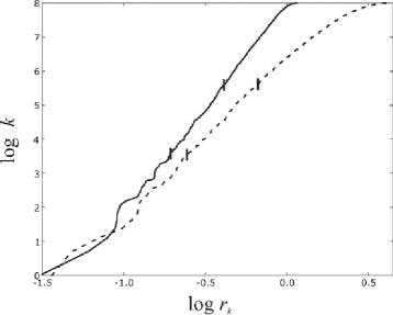
Figure 1: At the heart of the PD-E method is the determination of slopes in a log-log plot of the index of data points sorted by distance from a reference point as a function of that distance (referred to as an $r$-$V$ curve). The slopes indicate esimates of an exponent $d$ in a power-law relationship between the radius $r$ and the volume $V$ (approximated by the number of points $k$ in the ball $r$): i.e., $V\sim r^{d}$. $d$ is an estimate of the dimension of the set of points. This figure shows two such graphs for points randomly distributed in a 6-dimensional ball. The full line is the graph for a reference point at the centre of the ball, and the dotted line is the graph for a reference point with coordinates $(0.57,-0.14,-0.12,0.37,0.66,0.03)^{t}$. The marker lines on the graphs indicate a range within which PD-E selects the neighbourhood’s inner and outer radii and computes the slope of the secant defined by the two radii on this graph. The slopes for the central reference point and the distal reference point are 6.1 and 5.0, respectively. (Reference points near to the boundary of data sets are more likely to generate $r$-$V$ curves with lower slopes and thus cause the dimension of the sets to be underestimated.)

Among the sources of variability in the slopes of the $r$-$V$ curves are the following:

1. Sampling errors that reflect the difference between the data set and the probability measure $\mu$ it is assumed to approximate.

2. Noise in the data is expected to yield measures that are always $D$ dimensional, but the amplitude of the noise is likely to make the support of the measure “thin” in some directions.

3. The pointwise dimension of the measure $\mu$ may not exist, and even if it does, the slope of the log-log plots may have asymptotic slope $d$ only for $\mu$-almost all reference points. This is a typical situation for dynamical system attractors related to their multifractal structure [18].

4. The “shape” of the dataset and $\mu$ affects the slope of the log-log plot at larger distances from the reference point. As an example, the slope of the log-log plot for uniform measure on a two dimensional rectangle with side lengths $R_{1}\ll R_{2}$ will be approximately one for radii $R_{1}<r<R_{2}$. In high dimensional balls and rectangular solids, a very large proportion of the measure is concentrated near the boundary of the set, leading to slopes of the $r$-$V$ curves that are substantially smaller than the dimension.

In the absence of firm mathematical foundations for estimating pointwise dimension, we have pursued empirical tests on observational and simulated data. We have experimented with techniques for selecting a suitable “scaling” region of the $r$-$V$ curves that exclude small distances (smaller than $r_{x}^{min}$) subject to large sampling fluctuations and noise, and large distances (larger than $r_{x}^{max}$) where the global shape of the object plays a dominant role in determining the relationship between volume and radius. We have also experimented with ways of representing the statistical distribution of slopes with the scaling regions of $r$-$V$ curves. We assume that a random selection of a moderate number of reference points suffices to approximate the distribution of these slopes for the measure $\mu$. Unless otherwise stated we select $0.2N$ reference points.

Based on the above observations and assumptions we characterize the varying slopes of the $r$-$V$ curves in this paper in the following way. For the $r$-$V$ curve of each reference point $x$, we ignore the five points closest to the reference point, and the furthest 30%. With the remaining points, a range of secants are determined along the curve. The lower positions of the secants are selected at uniform intervals in the space of nearest neighbour indices, in steps of $0.0005N$ (rounded, if necessary). Thus, the lower point of contact on the $r$-$V$ curve for a secant with index $k$ is $\mathrm{log}\,(k)$. The upper index is chosen to be $\Delta k$, where we choose the constant $\Delta=4$ based on observing the typical scale of regions of near-constant slope on the curves. The upper point of contact is therefore $\mathrm{log}\,(\Delta k)$. The range of $k$ indices for secants ends where $\Delta k$ becomes equal to or greater than $0.7N$. The minimum and maximum of the slopes of the secants are recorded for reference point $x$, and are denoted $d_{x}^{0}$ and $d_{x}^{1}$, respectively. We then calculate the minimum, maximum, mean, median, and inter-quartile range of the sets $(\mathrm{min\ slopes})=\left\{d_{x}^{0}\right\}_{x}$ and $(\mathrm{max\ slopes})=\left\{d_{x}^{1}\right\}_{x}$ defined over the range of reference points $x$.

We plot representative $r$-$V$ curves for reference points corresponding to the extrema and the means of these sets. We also use a scatter plot of all $(d_{x}^{0},d_{x}^{1})$ pairs as a function of $x$ to characterize the distribution of slopes found. We highlight the points in the scatter plot corresponding to the extrema and means using a colour code. The full description of the graphical presentation of these statistics is given in the caption to Figure 6.

We also considered an alternative approach for assigning slopes to $r$-$V$ curves based on linear regression. That approach produced estimates of dimension within the range of the method described here. The determination of the slopes of secants requires fewer calculations than attempting to fit straight line segments on the $r$-$V$ curves using linear regression.

2.3 Computer generated synthetic data

We tested the PD-E algorithm on independent samples from measures of known dimension. The test measures we used are Lebesgue measure on 6- and 54-dimensional rectangular solids and balls. (The dimension of the space of motion capture marker data from our robot arm is 54, as there are 18 reflective markers placed on the robot.) We analyzed points uniformly distributed in a rectangular solid with sides of unit length, and from one that has 4 sides one fifth of the length of the remaining unit-length sides. This enables us to explore the fact that the relative length scales of different directions in the data are an issue for dimension estimation algorithms. We investigated sample sizes between 2,000 and 8,000 points.

We also performed tests of the algorithms involving the “Swiss roll” surface used as a benchmark by Tenenbaum et al. [7]. The Swiss roll is a two dimensional surface coiled smoothly in a three dimensional space. We generated one-dimensional curves on this surface parameterized by an angle $\theta$ (both closed and open curves), from which we uniformly sampled 1,000 points. Before rolling the two dimensional surface that contains the curve, the $(x,y)$ coordinates for the $i^{\mathrm{th}}$ of $N$ sample points were generated by the formulae $(0.5\,\mathrm{cos}\,\theta+b_{x}i/N,0.5\,\mathrm{sin}\,\theta+b_{y}i/N)$. For the closed curves, we set $(b_{x},b_{y})=(0,0)$, whereas for the open curves the values used were $(1.0,0.2)$. The transformation that rolled these points in the plane into three dimensions is given by $(x,y)\mapsto\left((1.5-1.4x)\,\mathrm{cos}\,4\pi x,y,(1.5-1.4x)\,\mathrm{sin}\,4\pi x\right)$. The relative scales of the Swiss roll manifold are set so that the curve extends approximately one quarter of the distance in the $y$ direction as in the $x$ and $z$ directions.

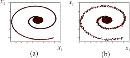
Figure 2: (a) and (b) A projection of points sampled randomly from a planar disc and points generated along a single spiral arm in the same plane, embedded in 5 dimensions. The disc consists of 2,000 points, and the spiral arm contains 1,000 points. In (b) Gaussian noise was added to all points.

In a third set of benchmark tests, synthetic data sets were generated by sampling from a set that is a union of two manifolds of different dimensions. This consisted of a planar disc region (with a radius of 1.8) and one or two spiral arms emanating from the disc in the same plane. See Figure 2. The spirals were generated as involutes of a circle having half the radius of the disc, using the relationship $r^{2}=\phi^{2}+1$ in polar coordinates, yielding an inter-arm distance of approximately twice the radius of the disc. The total diameter of the data set in the plane was approximately 18. 2,000 points were sampled from the disc and 1,000 from the spiral arm. These data were then embedded in a five-dimensional ambient space. In some tests Gaussian noise was added to all five coordinates with a standard deviation equal to approximately 5% of the radius of the disc. The range of the noisy data in directions orthogonal to the disc and spiral is approximately $\pm 0.5$, which is approximately 30% of the disc’s radius.

2.4 Motion capture data for robot arm

An AdeptSix 300 robot arm with six rotational joints was used to produce motion capture data. These data sets tested our analytical techniques on a real mechanical system whose active DOFs are known precisely. The motion of a robot arm is similar to a musculoskeletal system, but exhibits less noise and has no passive DOFs.

The “home” configuration of the robot arm can be seen in Figure 3. Figure 4 is a schematic diagram of the arm showing the local Euclidean coordinate frames defined around each link. The total length of the links is approximately 800 mm.

Three reflective markers were attached around each joint (see Figure 3) for the purpose of tracking the robot’s posture by a 4-camera optical motion capture system manufactured by Vicon (Vcams, Vicon Workstation). Table 1 provide details of the reflective marker positions using the local coordinate axes for the joints. Marker data were captured at a rate of 100 Hz. Only frames in which all markers were visible and properly reconstructed were kept in the final data set. The mean calibration residual of the Vicon marker reconstruction is less than 0.2 mm. The standard deviation in the reconstructed distance between two markers on a rigid object is approximately 0.05 mm.

 

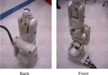
Figure 3: The “home” configuration of the AdeptSix 300 robot arm, showing the reflective markers used for 3D motion capture.

 

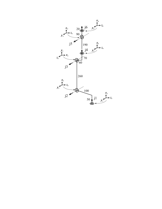
Figure 4: Schematic diagram of the physical dimensions of the robot arm (units are mm), including indication of joint axes and their local Euclidean coordinate frames (used for specifying marker positions).

Joint	Marker 1	Marker 2	Marker 3
1	(70, -100, 20)	(64, 100, 0)	(58, 100, -20)
2	(275, -120, 40)	(255, 110, 45)	(300, 110, 5)
3	(-120, 30, -55)	(-60, -30, -55)	(30, 15, -50)
4	(100, 75, 50)	(70, 75, 25)	(70, -85, -20)
5	(10, -30, 65)	(20, 30, 60)	(10, 30, -55)
6	(30, -35, 0)	(30, -20, -30)	(30, 32, 7)

Table 1: Approximate marker positions from joint axes in local Euclidean joint coordinates (units are mm).

Two experiments were performed with the AdeptSix 300. In the first, the robot arm was programmed to move to a succession of joint angles in a random walk that cyclically varies a single joint angle at each step. Conservative limits were placed on each angle choice to prevent the robot from hitting either the floor or itself during motion, and to keep all the markers within the range of visibility of the cameras. The constraints used on each joint were $\pm 30^{\circ},\pm 15^{\circ},\pm 15^{\circ},\pm 45^{\circ},\pm 15^{\circ},\pm 120^{\circ},$ respectively. The speed of robot movement was selected to expedite the trial times but the motion did not exhibit extraneous oscillations. The transition time between target postures was approximately $1/3\,s$.

An initial set of random angle displacements were selected. These were added to the angles associated with the robot’s default posture, and individually reselected when any of the angle limits were passed. This generated the first target posture of the robot. The next position was selected by randomly choosing the angular displacement of joint #1. The joint to be updated was cycled through the six joints for determining each subsequent posture. The distribution of points in joint space produced by this protocol is random, but may not be uniform.

The joint angle targets chosen in the first experiment were recorded so that exactly the same sequence of targets could be reproduced in a second experiment. The second experiment differed by putting the entire robot arm inside a tight elastic sheath (white hosiery, attached by elastic bands around joints 2 and 4), and re-attaching the markers in positions as close as feasible to their prior positions in the nominal configuration (see Figure 5). The sheath was intended to provide a source of systematic noise in the measurement of the robot’s actual motion, in this case to mimic the effects of skin in the reconstruction of animal skeletal motion using markers attached to the skin.

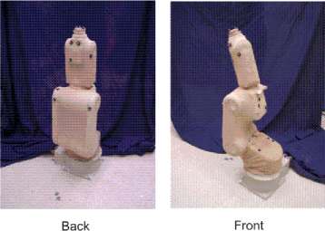
Figure 5: The sheathed robot arm and marker placement.

2.5 hours of data were collected from each experiment, but this was resampled at a rate of approximately 1 frame per three seconds, resulting in a data set of approximately 4,000 points.

We did not low-pass filter the kinematic data in our method so that we retained any correlated high-frequency components (“synergies”) of motion along with actual noise. It is a goal of our analytical methods to separate sources of noise and correlated high-frequency components.

2.5 Virtual robot motion

We further tested our methods with synthetic data of a simulated robot arm without an elastic sheath. We reconstructed the geometry of the AdeptSix 300 robot in a kinematic chain model of the joints, placing the same number of markers in approximately the same positions. The model was positioned by setting the six joint angles, and the forward kinematic transformation from angle space into Euclidean marker space was performed to generate marker positions of the virtual robot.

We used two different methods to generate joint angles of the arm. One method was the same random walk protocol used for the physical robot. The second was to use independent samples of a uniform measure in joint space. The same limits on the joint angles were used as for the physical robot. The chosen angles were mapped into marker space to obtain the data set.

The role of experimental measurement accuracy and noise can be investigated in the dimension estimation algorithms using the virtual robot. Also, different experimental protocols for selecting postures can be easily evaluated using simulations. The effect of limits on the joint angle selection on the output of the PD-E algorithm can be evaluated in the virtual domain because we can safely remove them and allow the virtual arm’s motion to be unconstrained by self-intersections of the robot arms or intersections with the floor. Additionally, there are issues as to the relative scales of the marker-axis distances for the different joints, which we would like to be able to vary in order to explore its effect on a dimension estimate calculation. The virtual robot allows us to position the markers arbitrarily around the axes.

2.6 Constrained hand motion

We used the Vicon 3D motion capture system to record time-series kinematic data of two subjects asked to perform three tasks. The subjects held their wrists in a fixed position while moving their fingers. Five reflective markers were placed on each finger (one at the fingertip and two between each of the joints), three on the thumb, and four additional markers were placed on the back of the hand (a total of 27 markers).

The first task was simultaneous “random” movement of their fingers close to the plane of the palm. The other two tasks were the simulation of typing on a computer keyboard and the simulation of manipulation of a track ball, both while keeping the wrist in a fixed position. These tasks were performed for approximately 20 minutes in four 5 minute segments, and the resulting data sets combined and resampled to select 3 frames per second. This resulted in final data sets containing approximately 8,000 points.

3 Results

3.1 Computer generated synthetic data

We expect that Isomap and PCA will detect that dimension reduction is inappropriate for data sampled randomly from Lebesgue measure on a sphere or rectangular solid in $\mathbb{R}^{D}$. We tested data sets of independent random samples from a 6-dimensional unit ball, using sample sizes of 2,000, 4,000, and 8,000. PCA at the 90% variance capture threshold determined $d=6$. Also, graphs of PCA residuals and Isomap residual variances showed no “knees,” indicating that using PCA or Isomap in this manner predicts that dimension reduction is not appropriate, as expected. However, PCA at the 80% variance capture threshold determined $d=5$, implying that for a sufficiently low threshold this use of PCA incorrectly predicts that dimension reduction is appropriate.

Figures 6 and 7(a)–(c) summarize the results of the PD-E analysis on the balls. The dimension was accurately estimated by the median of the maximum slopes of $r$-$V$ curves.

We compare these results with an analysis of 2,000 points drawn randomly from a 6-dimensional unit cube. The output of PD-E is shown in Figure 8(a), and corresponding statistics also appear in Figure 7. (The results were almost identical for $N=4000$.) The PCA results at 80% and 90% variance capture thresholds determined $d=5$ in both cases. The distribution of maximum slopes $d_{x}^{1}$ is very similar between the cube and the ball, but the minimum slopes $d_{x}^{0}$ are more widely spread for the cube. From the $r$-$V$ curves plotted, the minimum slopes appear to be found at larger $r_{x}$, which is where we expect the most distortion due to boundary effects of the set. These effects are seen even more strongly in Figure 8(b) for the 6-dimensional rectangular solid with four sides having one fifth the length of the remaining two. Again, the minimum slopes are found mostly at larger $r_{x}$ and their distribution is more dispersed than that of the maximum slopes.

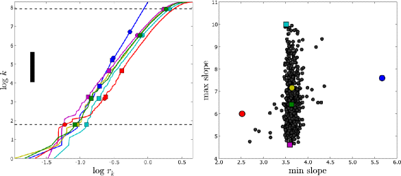
Figure 6: PD-E analysis of a uniformly-random distribution of sample points from a 6-dimensional unit ball. The left panel shows $r$-$V$ curves for the colour-coded points in the scatter plot in the right panel. These highlighted points indicate the minimum, maximum and mean of the minimum and maximum slopes. Round markers indicate statistics relating to the minimum slopes, square markers relate to the maximum slopes. The colour coding is as follows: red = minimum of $(\mathrm{min\ slopes})$; yellow = mean of $(\mathrm{min\ slopes})$; blue = max of $(\mathrm{min\ slopes})$; magenta = min of $(\mathrm{max\ slopes})$; green = mean of $(\mathrm{max\ slopes})$; cyan = max of $(\mathrm{max\ slopes})$. We define $(\mathrm{min\ slopes})=\left\{d_{x}^{0}\right\}_{x}$ and $(\mathrm{max\ slopes})=\left\{d_{x}^{1}\right\}_{x}$. The secant end points estimating the minimum and maximum slopes of all the $r$-$V$ curves plotted are indicated by round and square markers, respectively. The dotted lines mark the closest and furthest nearest neighbours considered in the estimation of slopes. The solid bar indicates the size of the free parameter $\mathrm{log}\,\Delta$. The broad distribution of maximum slopes in the scatter plot can be largely attributed to the distance of the associated reference point $x$ from the centre of the ball.

 

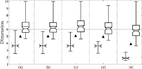
Figure 7: PD-E dimension estimates for a uniformly-random distribution of sample points from a 6-dimensional solid: (a) a unit ball with $N=8000$, (b) a unit ball with $N=4000$, (c) a unit ball with $N=2000$, (d) a unit cube with $N=2000$, and (e) a rectangular solid having 2 sides of unit length and 4 sides of length 0.2, with $N=2000$. For each solid, two box-and-whisker plots are shown. The left plot indicates the distribution of $(\mathrm{min\ slopes})$, the right indicates that of $(\mathrm{max\ slopes})$. In each case, the whiskers mark the extent of the data (from minimum value to maximum), the boxes mark the inter-quartile range. The notches indicate the median value. The horizontal line in the box indicates the mean value. When the inter-quartile range is very small, the top and bottom of the box is not drawn for the sake of clarity: the range is still apparent by the distance from the median to the beginning of each whisker. The black triangle between each pair of box plots indicates the mean of the data from $(\mathrm{min\ slopes})$ and $(\mathrm{max\ slopes})$ taken together. The thin horizontal line across each panel indicates the known dimension $D$ of the data set analyzed. Panels (a)–(c) show the relative insensitivity of PD-E results on the number of points in the data set. Panel (d) shows that the data set’s non-smooth boundary does not significantly affect the results, compared to the smooth boundary in (c). Panel (e) shows that the relative scales of the solid’s side lengths distort the distribution of PD-E dimension estimates.

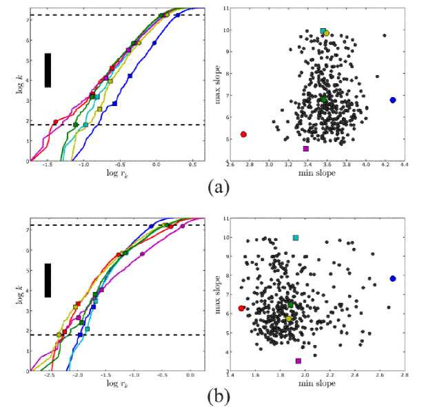
Figure 8: Output of the PD-E algorithm for the uniform random data sampled from a 6-dimensional rectangular solid with (a) equal side lengths, and (b) 4 sides one fifth the length of the other 2. In (b) the slopes of the $r$-$V$ curves can be seen to flatten out for $\log\>r_{k}>-1$, a result of balls $B_{x}(r)$ growing outside the solid in the shorter directions for lower values of $r$.

Figure 9 shows the graphs of PCA residuals for points sampled from rectangular solids with $D=54$. For a rectangular solid with unequal side lengths, a knee was detected in the graph of PCA residuals at $d=50$ that reflects the decreased variance of the data in four directions. At the 80% and 90% variance capture levels PCA estimated the dimension of the 54-dimensional rectangular solid with equal (unequal) sides to be 42 and 48 (39 and 45), respectively.

In order to apply Isomap we down-sampled these data sets by a factor of one half, to fit the size limitations of the current implementation of Isomap. Using $K=50$ we obtained the distribution of residual variances as a function of embedded dimension shown in Figure 10. Similar results were obtained for larger values of $K$, and values of $\varepsilon>4$. The knees of these distributions correspond to 54 for the rectangular solid with equal side lengths and 50 for the solids with four shorter sides.

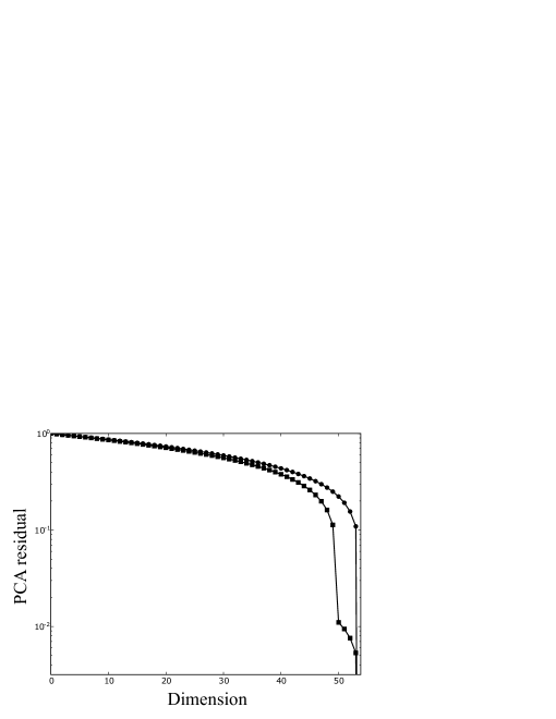
Figure 9: Linear-log plot of PCA residuals as a function of embedding dimension, for data set from 54-dimensional rectangular solid with equal side lengths (round markers) and with 4 sides one fifth the length of the other 50 (square markers). A knee is detected in the latter at $d=50$. The commonly-used criterion for choosing the estimated dimension $d$ in PCA uses a pre-selected “variance capture” threshold, which leads to sensitivity of the estimates to noise variance and generally an underestimation of dimension. In contrast, the detection of knees in this linear-log graph of the residuals performs more reasonably. Here, it correctly predicts that dimension reduction is not appropriate for the 54D solid with equal side lengths (no knee), although it incorrectly predicts that a mild reduction to $d=50$ is appropriate for the 54D solid with unequal side lengths.

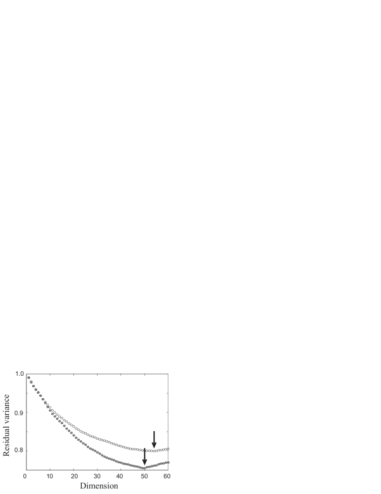
Figure 10: Plot of residual variance from Isomap embeddings ($K=50$) applied to data sampled from a 54-dimensional rectangular solid with equal side lengths (open circles), and a 54-dimensional rectangular solid with 4 sides one fifth the length of the other 50 (solid circles). The arrows indicate the positions of the minima in the plots corresponding to the best estimate of dimension of the data set. The detection of knees in these graphs as an indication that dimension reduction is appropriate correctly predicts that it is not appropriate for the 54D solid with equal side lengths, although it incorrectly predicts that a mild reduction to $d=50$ is appropriate for the 54D solid with unequal side lengths. Isomap’s performance on these sets are essentially the same as that of PCA using the knees in the graphs of residuals (Figure 9).

PD-E analysis of these 54-dimensional examples gives results that require more complex interpretations. As $N$, the number of sample points, increases, the $r$-$V$ curves show the volumes of balls intersected with the region $R$ from which the samples are drawn. When the radius of the ball exceeds the distance from the reference point to the boundary of $R$, the slope of the $r$-$V$ curve decreases. In high dimensions, most of the measure of a sphere or rectangular solid is concentrated close to its boundary since volume grows proportionally to $r^{D}$. Also, the smallest interpoint distance that we expect to find in a data set of $N$ points increases with dimension. Thus we expect that the slopes computed from the $r$-$V$ plots will underestimate $D$.

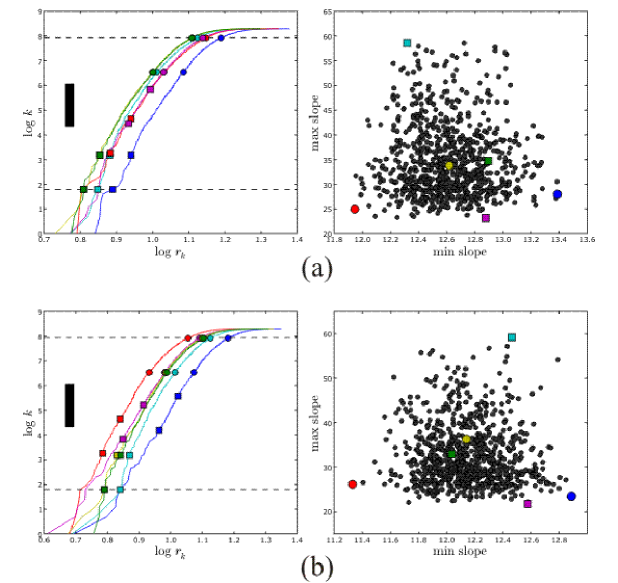
Figure 11: PD-E analysis for the uniform random data sampled from a 54-dimensional rectangular solid having (a) equal side lengths, and (b) 4 sides one fifth the length of the other 50. The flattening out of slopes in the $r$-$V$ curves for larger radii $r_{k}$ is less apparent for the solid with 50 long sides and 4 short sides in (b), compared to the 6D solid in Figure 8 where there are only 2 long sides compared to 4 short sides.

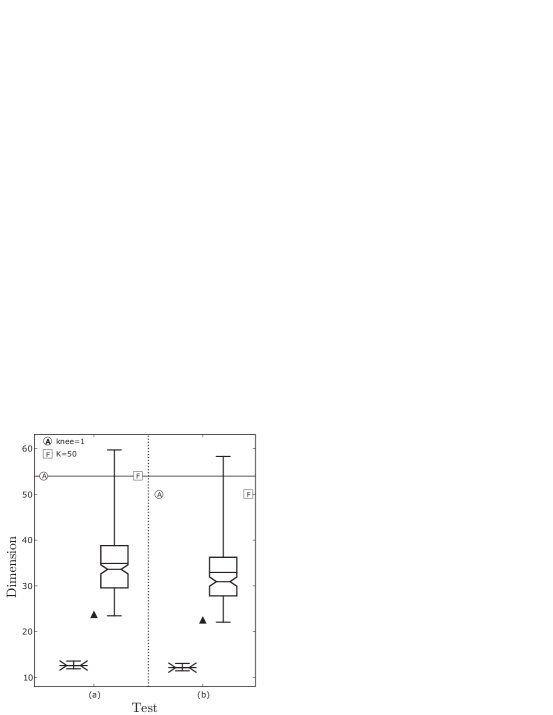
Figure 12: Dimension estimates of 54-dimensional rectangular solids having (a) equal side lengths, and (b) 4 sides one fifth the length of the other 50. A description of the box-and-whisker plots is given in Figure 7. The circular markers indicate the dimension estimation result for PCA using the first knee of the residual. The square markers indicate the dimension estimation results for Isomap using the parameter indicated. For such high-dimensional sets PD-E does not accurately predict $D$ but still provides a reasonable upper bound on the dimension.

We tested the algorithms on a curve of points lying on a Swiss roll manifold to assess their ability to estimate the dimension of a highly nonlinear and low-dimensional manifold. In Figure 13(a) the points are evenly distributed on a closed curve and the sampling is noiseless. In Figure 13(c) the curve is open, and Gaussian noise was added with zero mean and a standard deviation of 0.02 (corresponding to about 4% of the spatial separation between the layers of the rolled manifold).

The results of the PD-E analysis of the closed curve data set are shown in Figure 14(a). The statistics corresponding to these are given in Figure 15. There is a clear clustering in the scatter plot of minimum and maximum slopes that corresponds to large and small radii in the $r$-$V$ curves. Balls of small radius intersect a single branch of the curve and volumes increase linearly with $r$. Balls of larger radius intersect an increasing number of branches of the curve and display an increase in volume that is faster than linear, reflected in the larger slope of the $r$-$V$ curves. For the open curve with added noise the output of the algorithm shows some dispersal of the cluster of points associated with $d_{x}^{0}\approx 1.1$ along the axis of minimum slope (Figure 14(b)), but little dispersal of the cluster associated with $d_{x}^{1}=3$ along the other axis. This is to be expected because the amplitude of the noise is small compared to the global extent of the curve in the three-dimensional space.

PCA at a threshold of 80% and 90% variance capture identified 2 dimensions for both the noise-free and noisy data sets. In Isomap we set the $\varepsilon$ parameter to be a length scale known to be much smaller than the distance between the rolls of the surface ($\varepsilon=0.08$). The residuals for embedding in dimensions 1, 2, and 3 for the noise-free data were $1.4\times 10^{-7}$, $7.8\times 10^{-6}$, and $2.1\times 10^{-5}$, respectively, indicating a minimum immediately at $d=1$. The residuals for the noisy data were $3.1\times 10^{-4}$, $1.9\times 10^{-4}$, $4.2\times 10^{-4}$. Therefore, Isomap estimates $d=1$ for the noise-free data and 2 for the noisy data. However, if greater length scales are used for $\varepsilon$ then the residual variance for $d=1$ becomes approximately a magnitude larger than for $d>1$, meaning that Isomap estimates $d=2$ in both cases. Using the alternative control parameter $K$, Isomap only detected $d=1$ for these data sets for $K$ between 5 and 15.

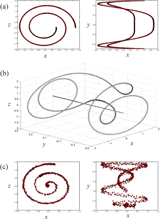
Figure 13: (a) A sample of 1,000 points from a closed curve embedded on a Swiss roll manifold, projected in to the $(x,z)$ and $(x,y)$ planes. (b) 3D projection of the curve in panel (a) showing the central axis of the roll along $(x,z)=(0,0)$. (c) A noisy sample of 1,000 points from an open curve on a Swiss roll manifold, shown in the same projections as panel (a). Note that the $y$-axis scaling is one quarter that of the other axes.

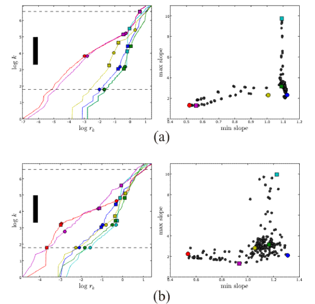
Figure 14: (a) PD-E analysis for the closed curve on a Swiss roll manifold. (b) PD-E analysis for the open curve on a Swiss roll manifold with added Gaussian noise. The minimum slopes of $r$-$V$ curves occur most typically for small radii $r$, whereas the maximum slopes occur most typically for large radii. At the smaller scales (smaller $r$) the minimum slopes are clustered near the known dimension of the curve, $d_{x}^{0}=1$. At larger scales (larger $r$) the maximum slopes $d_{x}^{1}$ detect the dimension of the 3D ambient space in which the curve is embedded.

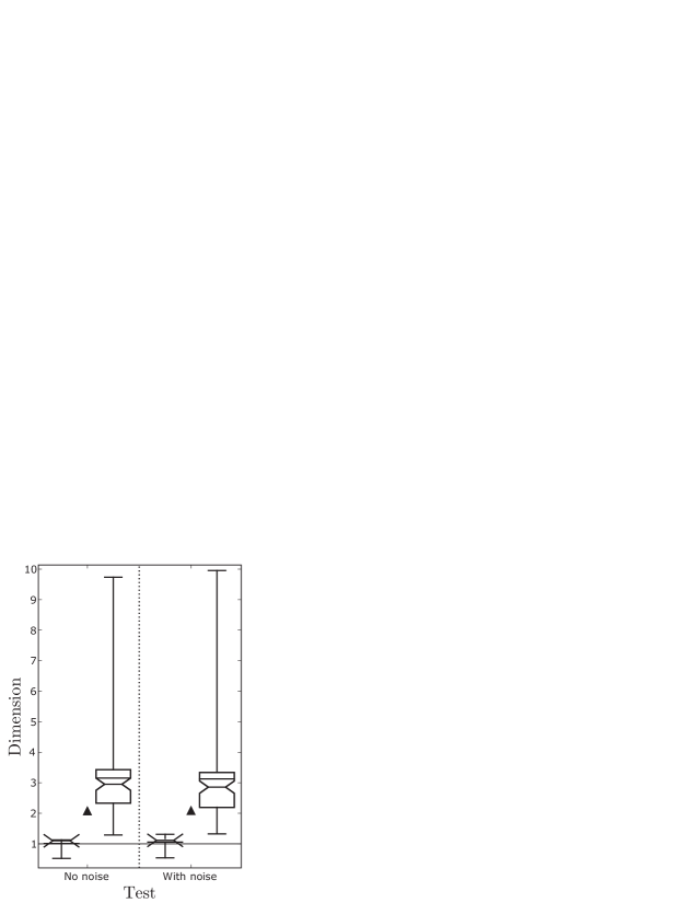
Figure 15: PD-E estimates for curves lying in the Swiss roll manifold. A description of the box-and-whisker plots is given in Figure 7. The presence of noise does not substantially alter the dimension estimates.

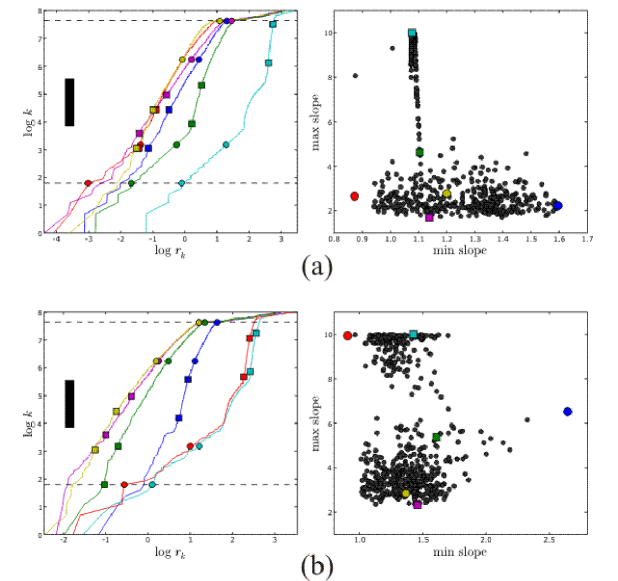
Figure 16: PD-E analysis for the data set sampled from the union of a disc and a co-planar spiral embedded in a 5-dimensional space. (a) No noise added. (b) Gaussian noise added with zero mean and a standard deviation of 0.1 in each of 5 dimensions. The clustering in the distribution of maximum slopes into two major concentrations is due to the data set being heterogeneously distributed in its ambient space (see text for details).

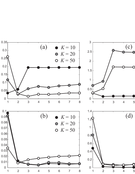
Figure 17: Graphs of Isomap residual variance versus embedding dimension $d$ for the data set sampled from the union of a disc and a co-planar spiral embedded in a 5-dimensional space. (a) Control parameter $K$, no noise added. (b) Control parameter $K$, noise added. (c) Control parameter $\varepsilon$, no noise added. (d) Control parameter $\varepsilon$, noise added. The vertical scales are not equal between parameter values, but only the relative change of each graph of residual variance as a function of $d$ is important. These graphs show that the estimate $d$ is more sensitive to the parameter value $K$ than to $\varepsilon$, as the knees or minima in the residual variances as a function of $d$ vary between 2 and 4 when $K$ is varied.

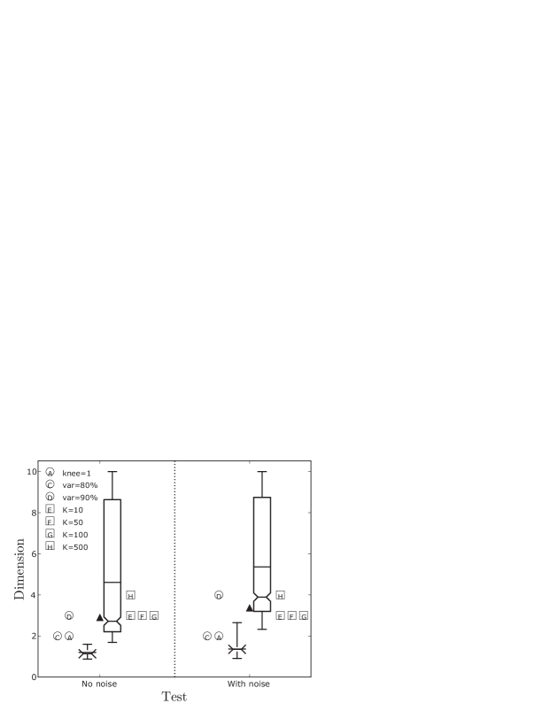
Figure 18: PD-E estimates for the data set sampled from a planar disc and spiral embedded in a 5D ambient space. A description of the box-and-whisker plots is given in Figure 7. The circular markers indicate the dimension estimation results for PCA using the method indicated. The square markers indicate the dimension estimation results for Isomap using the parameter indicated. Additional values of $\varepsilon$ were tried that are not marked in this figure, giving estimates of $d=2$ (see Figure 17). The broad distributions of maximum slopes are due to the data set being heterogeneously distributed in its ambient space (see text for details).

In Figures 16 and 18 a PD-E analysis of the disc-with-spiral data set indicates the presence of two manifolds with different dimension, with two markedly different groupings of slopes of $r$-$V$ curve corresponding to $d=1$ and $d=2$. We make four observations about this analysis.

(1) For reference points in the spiral arm, such as those for the cyan or green $r$-$V$ curves, the slopes at small radii are approximately one. Sharp increases in slope are observed at moderate distances corresponding to balls reaching the central disc or other parts of the spiral. As such a contact is made a ball will suddenly encounter a large density of points over a relatively small increase in radius, and thus the “volume” approximated by $\log(k)$ will increase at a higher rate as $r$ increases. This effect gives rise to secants in the cyan and green $r$-$V$ having a spread of maximal slopes $d_{x}^{1}\sim 10$ that do not correspond to the dimension of any manifold. When the balls increase in radius by the size of the disc’s diameter the slopes in the $r$-$V$ curves again suddenly flatten out. For comparison, a PD-E analysis was repeated on the spiral arm part of the data set. This produced a scatter plot that only retained the cluster of points lying along the vertical axis at $d_{x}^{0}\approx 1.05$ (data not shown), confirming that the disc was entirely responsible for the slopes clustered at $d_{x}^{1}\approx 2$.

(2) For reference points inside the disc, such as that for the yellow $r$-$V$ curve, $k(r)\sim r^{2}$ (indicated by $d_{x}^{1}$) until the ball radii reach the edge of the disc at a radius of 1.8. For the yellow curve with $x=(-0.186,-0.464)^{t}$ this happens at approximately $\log(r)=\log(1.8-|x|)\approx 0.26$. After the edge is reached, balls grow at a lower rate, which fluctuates as the balls reach successive parts of the spiral arm. From the plotted $r$-$V$ curves, the spread of minimum slopes $d_{x}^{0}$ corresponds to balls centred in the disc having large enough radii that they are not fully contained inside the disc.

(3) The summary statistics for the PD-E analysis in Figure 18 do not adequately represent the bimodal nature of the distribution of $r$-$V$ curve slopes shown in Figure 16.

(4) The added noise had sufficient amplitude in directions orthogonal to the plane of the disc and spiral to increase the estimated dimension by approximately 0.6, as seen in the increase of $\min\>(\mathrm{max\ slopes})$ and $\mathrm{mean}\>(\mathrm{max\ slopes})$ in Figure 18.

The results of Isomap for the disc and spiral data set are shown in Figure 17. In the absence of added noise in the data sets, Isomap estimated a single two- or three-dimensional manifold for the disc-with-spiral data set for $K\geq 15$. Isomap was very sensitive to the choice of $\varepsilon$, and failed except at $\varepsilon\approx 0.1$ (0.25) for the noise-free (noisy) data, when it estimated $d=2$ (3). The addition of noise to the data set otherwise made little difference to the estimates of $d$. The neighbourhood graphs generated typically contained only one connected component, but any additional components found contained too few points to be embedded separately. PCA at 80% and 90% variance capture thresholds esimated $d=2$ for both the noise-free and noisy data sets, while the estimate from the position of a knee in the graph of PCA residuals was $d=2$ (3) for the noise-free (noisy) data.

3.2 Virtual robot arm data

In a marker configuration corresponding closely to that of the physical robot, 4,000 frames of randomly generated virtual robot arm postures were analyzed. We first consider the method of joint angle generation that randomly samples the absolute joint angles from a uniform distribution. The results of this are presented as Test 1 in Figure 20, and the corresponding $r$-$V$ curves and scatter plots from PD-E are shown in Figure 19(a).

The last rigid link in the robot arm is both short (approx. 30 mm) and narrow (approx. 60 mm). Therefore, the typical distance of the three markers around the associated joint (#6) from the joint axis is small in comparison to those at the other joints. We investigated the effect of these multiple spatial scales on the dimension estimation algorithms by moving the marker positions on the virtual robot further from the centre of joint 6. The more widely spaced positions of the markers around joint 6 were (30, -75, 0), (30, -40, -40), (30, 65, 15) in the respective local coordinate frames. These are distributed at a spatial scale comparable to the markers around joint 5. The output of PD-E for this marker configuration is shown in Figure 19(b), and the dimension estimate statistics are presented as Test 2 in Figure 20. Isomap gave similar results when varying $\varepsilon$ between 80 and 400. A further widening of the marker spacing from the joint by 50% primarily reduced the inter-quartile range of the PD-E slope estimates (data not shown). Figure 21 graphs the residuals of PCA $d$-dimensional embeddings of three virtual robot motion data sets as a function of the number of components $d$.

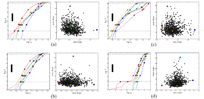
Figure 19: PD-E analysis for (a) the original virtual robot marker placement, and (b) with more widely spaced markers at joint 6. The position of joint 3 is slaved by that of joint 2 in (c) for the original marker placement. (d) In contrast to the uniform distribution of joint angles used in (a)–(c), this plot shows the results for joint angles determined by a random walk in joint angle space, using the original marker placement. Almost flat regions of some $r$-$V$ curves are observed in (d) for small radii, corresponding to the presence of localized clusters of a few closely-spaced points. The $r$-$V$ curves in all the plots flatten out slightly at the largest radii, presumably as balls $B_{x}(r)$ extend outside the data set in some directions but not others.

We performed two further tests with the original marker configuration. In Test 3, we slaved the position of joint 2 to be a smooth function of the position of joint 3, according to $\theta_{2}=\theta_{3}^{3}$. In Test 4, we simply froze the position of joint 3. The number of DOFs of the system are reduced by one in each case. The PCA and Isomap results for these two tests are identical, and the PD-E results for the two tests were almost identical. For this reason only the statistics for Test 3 are listed in the table.

The virtual setting for the simulated robot arm permitted us to explore the effect of physical constraints on the dimension analysis of the physical robot arm’s motion. The primary constraints are the presence of the floor to which the robot is attached and the limited field of view of the motion capture video cameras. These constraints are easy to remove in the simulations, and in Test 5 we generated 4,000 frames of postures for the original marker configuration, in which joint angles were chosen randomly throughout their full $360^{\circ}$ range. (This corresponds to an underlying measure without boundary.) We observe that the PD-E dimension estimates for this data set did not change by more than a few percent compared to Test 2, but the PCA and Isomap algorithms estimated one dimension greater across the same range of $K$ and $\varepsilon$ values.

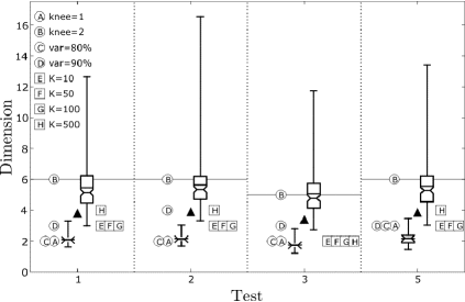
Figure 20: Dimension estimates of virtual robot data sets consisting of 4,000 frames. Test 1 uses the original marker placement. Test 2 uses a configuration in which markers were spaced more widely around joint 6. In Test 3, the position of joint 2 is slaved to be a smooth function of the position of joint 3. (Test 4 results are omitted.) Test 5 removes the physically-realistic constraints on joint angles present in the other tests. A description of the box-and-whisker plots is given in Figure 7. The circular markers indicate the dimension estimation results for PCA using the method indicated. The square markers indicate the dimension estimation results for Isomap using the parameter indicated. The results indicate that PCA using a variance capture threshold consistently underestimates $D$. PD-E , Isomap, and PCA (using residual variances) all succesfully detected that the dimension of the set in Test 3 is one lower than in the other tests. PD-E provides a good estimate near to the mean of the data set for $(\mathrm{max\ slopes})$. The additional widening of marker placement in Test 2 did not qualitatively affect the estimates, although it made the mean and median $(\mathrm{max\ slopes})$ values from PD-E more accurate. Test 5 demonstrates that the constraints on arm position make little difference to the dimension estimates.

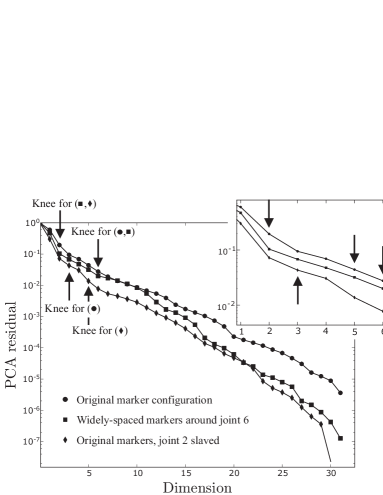
Figure 21: Residuals of $d$-dimensional PCA embeddings of the virtual robot motion data. The positions of the first two knees in the graphs are indicated by the arrows. The inset shows the region of the graph around the positions of the second knees.

We studied the dependence of the analyses on the number of points $N$ in the data set by reducing $N$ from 8,000 to 4,000, 2,000, and 1,000, for the widened configuration of the markers at joint 6 on the simulated robot. Figure 22 presents a comparsion of the results using the different methods. For this range of $N$ we did not observe an effect on the position of knees in the graph of PCA residuals.

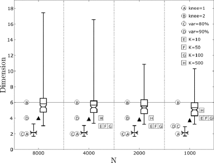
Figure 22: Dimension estimates of virtual robot data sets (with more widely spaced markers on joint 6) as $N$, the number of points in the set, is varied. A description of the box-and-whisker plots is given in Figure 7. The circular markers indicate the dimension estimation results for PCA using the method indicated. The square markers indicate the dimension estimation results for Isomap using the parameter indicated. The mean and median values of $(\mathrm{max\ slopes})$ in the PD-E distributions become less accurate as $N$ is reduced, but the spread of the distributions also tightens. Isomap also became inaccurate as $N$ decreased to 1,000. PCA results were almost unaffected by the changes in $N$, and the estimation of $D$ using the second knee in the residuals was correct in every case. (Note that Isomap could not be run for $N=8000$ because the data set was too large for the inter-point distance matrix to be calculated.)

We next generated data for the virtual robot arm by performing a random walk in joint angle space. The results of this are presented in Figure 19(d). One major difference in these results is the presence of $r$-$V$ curves with very flat regions. These regions cause the distribution of minimum slopes $d_{x}^{0}$ to include values near zero, and as these regions contain so few points their slopes are not interpreted as dimension estimates. The initially steep rise of $\log(k)$ as a function of $r_{k}$ before a flat region suggests that there is a small cluster of data points that are very closely spaced in comparison with the typical distances between other points in the data set. The cluster need not be spatially dislocated from the remaining points, and in this example we verified that the centres of the dense clusters are indeed located at distances comparable to the mean interpoint distances between all points in the data set. Thus, the presence of the flat regions in these $r$-$V$ curves may be due to the fractal structure of random walks and the low dimension of Brownian sample paths [19].

3.3 Robot arm motion and the exploration of “skin” artifact

Figures 23, 24, and 25 show the results of our analysis of the robot motion capture data. The mean values of the maximum and minimum slopes are close to those predicted from the virtual robot tests, and the qualitative pattern of point distribution in the scatter plots is similar to that in the virtual robot results when the method of joint angle generation is the same (see Figure 19(d)). The addition of an elastic sheath to the robot did not significantly change the dimension estimates, and in particular made almost no difference to the inter-quartile ranges of $(\mathrm{min\ slopes})$ or $(\mathrm{max\ slopes})$.

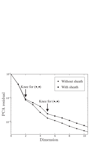
Figure 23: Residuals of $d$-dimensional PCA embeddings of the robot motion data.

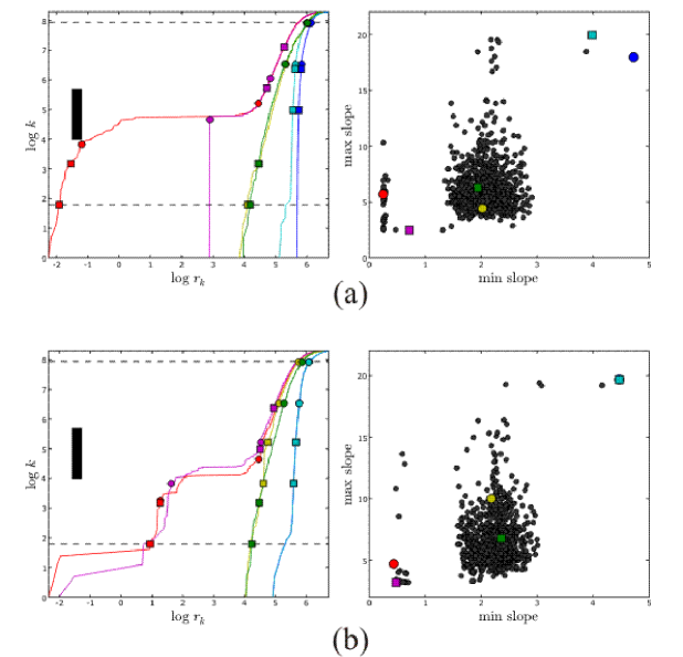
Figure 24: PD-E analysis of 4,000 frames of data for (a) the robot arm without the elastic sheath, and (b) the robot arm covered with the sheath. Notice that in the scatter plot for (b) the blue circle and cyan square coincide.

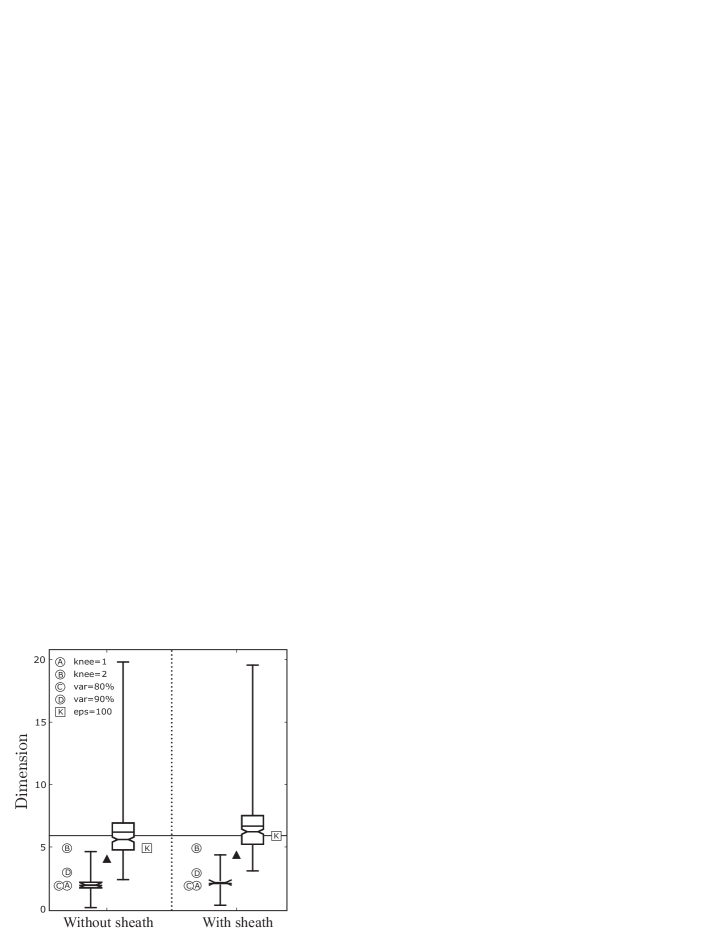
Figure 25: PD-E analysis of robot data sets with and without an elastic sheath, using $N=4000$. A description of the box-and-whisker plots is given in Figure 7. The circular markers indicate the dimension estimation results for PCA using the method indicated. The square markers indicate the dimension estimation results for Isomap using the parameter indicated. The addition of the sheath did not greatly increase the dimension estimates by any of the methods.

3.4 Hand motion

Our analysis of four data sets for human hand motion is given in Figures 27 and 29. The PCA residuals for these data sets are plotted in Figure 26. The most evident result is that all the methods estimate the dimension of hand motion to be less than 11, and probably around 6. Also, a histogram of the minimum slopes $d_{x}^{0}$ for the trackball task indicates the absence of a dense cluster at $d_{x}^{0}\approx 3$ in contrast to the other data sets (Figure 28). This may indicate that the appropriate dimension reduction for hand motion may be task dependent, but requires a more systematic analysis with more data.

In the scatter plots we observe a large number of points for which $\min\>(\mathrm{min\ slopes})\approx 0.5$. The red $r$-$V$ curves corresponding to the minimum $d_{x}^{0}$ secant slopes indicate that these are due to flat regions of the curve. In the study of the synthetic data sets we previously identified such flat regions as corresponding to localized subsets of a small number of closely-spaced points. In this case there appear to be many such small subsets. (Recall that these flat regions are due to this localization and that the associated low slopes are not indications of low dimension.) It will be instructive in future work to identify which hand postures are associated with these subsets.

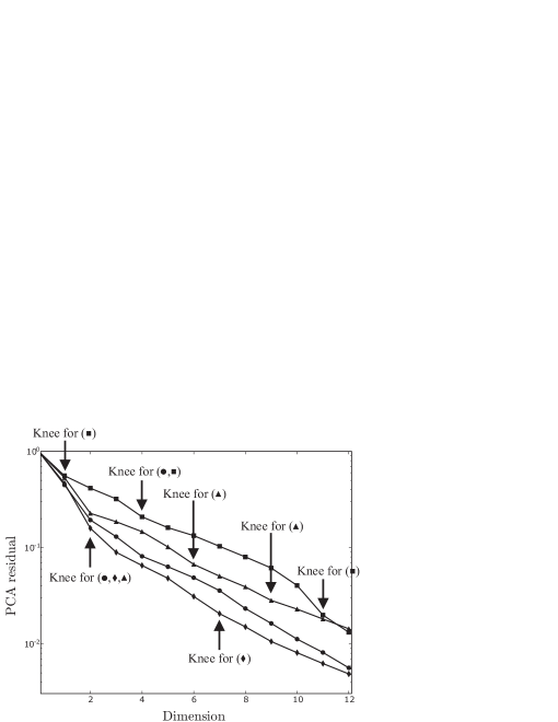
Figure 26: PCA residuals for all hand motion tasks, showing first two knees for each task. Random motion task (subject S2): circle markers; (subject S1): square markers. Keyboard task (subject S2): triangle markers. Trackball task (subject S1): diamond markers.

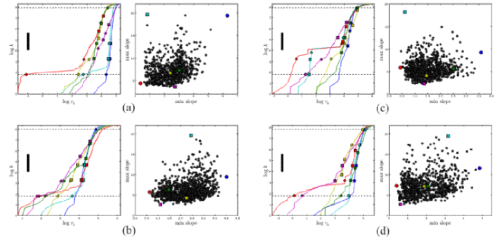
Figure 27: PD-E analysis for 4,000 frames of hand motion data. (a) Random motion task (subject S1).(b) Random motion task (subject S2). (c) Trackball simulation task (subject S1). (d) Keyboard simulation task (subject S2). Notice the presence of flat regions in the some $r$-$V$ curves for every task, and the mild flattening of the curves for radii $r>5$.

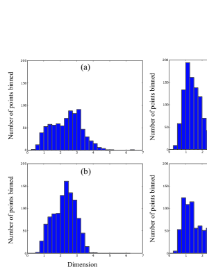
Figure 28: Histograms of minimum slopes $d_{x}^{0}$ with bin width 0.25 for the hand motion tasks. (a) Random motion task (subject S2); (b) Random motion task (subject S1); (c) Keyboard task (subject S2); (d) Trackball task (subject S1). These histograms show the roughly bimodal nature of the minimum slopes for all but the trackball task in (c), which appears to contain only a component centred at $d\approx 1$.

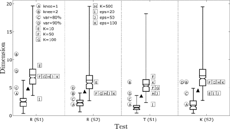
Figure 29: Dimension estimates of hand data sets from a sampling of 4,000 points. Task R: Random motion. Task T: Simulation of trackball manipulation. Task K: Simulation of computer keyboard use. A description of the box-and-whisker plots is given in Figure 7. The circular markers indicate the dimension estimation results for PCA using the method indicated. The square markers indicate the dimension estimation results for Isomap using the parameter indicated. Qualitatively, both PCA and Isomap predict estimates less than $d=10$. Most of the PD-E estimates are also in this range, although there are a few maximum slopes at higher $d$ values. There is not a clear quantitative trend in the estimates as a function of the task in this preliminary study using only two subjects.

4 Discussion

Motion capture data produces measurements of marked positions of an object in a $D$-dimensional data space. The number of kinematic degrees of freedom (DOFs) of the object is often substantially smaller than $D$, and the system may be constrained to a set of even smaller dimension than those which are kinematically feasible. In response to a growing trend in biomechanical and neurophysiological analysis to estimate the number of DOFs of a system (i.e., its “dimension”) using linear methods such as PCA, we compared PCA to two nonlinear methods (Isomap and the novel pointwise dimension estimation (PD-E ) algorithm) that are also designed for this purpose. We compared and contrasted the dimension predictions by the three methods using simulated kinematic data, and motion capture data from a robot arm and from human hands whose degrees of freedom are known and unknown, respectively. Additionally, we challenged the idea that a method such as PD-E , that is based on calculations of a type of fractal dimension, requires unreasonably large amounts of data.

We now summarize conclusions about the three methods of dimension estimation, followed by a discussion of the results for the tests on hand motion.

4.1 Interpretation of the pointwise dimension results

The PD-E algorithm assumes that the data set is a discrete approximation of a probability distribution and seeks asymptotic power law relationships of the form $V\sim r^{d}$ for the volumes $V$ of balls as measured by this distribution and their radii $r$. The log-log plots of $V(r)$ vs. $r$, which we refer to as $r$-$V$ curves, show this relationship for balls with a common center. The calculation of these curves is easy, but deriving an estimate for $D$ from these curves encounters several issues that complicate the analysis. Statistical sampling fluctuations and noise make estimates of $V(r)$ unreliable for small values of $r$, and the scaling relationship may break down for large values of $r$. Therefore, implementation of the methods seeks an intermediate “scaling region” in which the $r$-$V$ curves are approximately linear in log-log plots. At present there is not a complete analytical framework for applying the definition of pointwise dimension to experimental data in this way. As a first step, therefore, we have adopted an empirical approach to testing whether our PD-E algorithm provides reasonable estimates with data sets of a few thousand points approximating measures of known dimension.

The above complications to reliably estimating the volumes of balls using $r$-$V$ curves mean that PD-E analysis results in a statistical distribution of dimension estimates. This distribution requires interpretation by the user in the context of the experimental system and the quality and quantity of data. Primarily, the distribution provides an upper bound on the estimated dimension, and sometimes a lower bound if the lower end of the distribution tails off at a value greater than 1.

For smooth measures supported on manifolds with boundary we have found that the method produces a distribution of slopes for the $r$-$V$ curves whose upper bound is close to the known pointwise dimension of the measure. Typically, the slopes of the $r$-$V$ curves are smaller than the pointwise dimension of the underlying measure due to “boundary effects.” As the dimension of the manifold grows, an increasing proportion of points of the manifold lie near the boundary. Increasing dimension limits the radii of balls that do not intersect the manifold boundary. Simultaneously, statistical sampling fluctuations for balls of a fixed radius increase.

For measures that were intrinsically high dimensional (such as independent samples from rectangular solids), the distribution of slopes measured from the $r$-$V$ curves tends to cluster at values intermediate between $D/2$ and $D$. (For instance, this can be seen in the histograms of binned $d_{x}^{1}$ values for the 54-dimensional rectangular solids, in Figure 30.) The mathematical analysis of the disparity between $D$ and the slopes of the $r$-$V$ curves warrants further study.

However, in the tests on low-dimensional data sets of known dimension, one or other of the median values of $(\mathrm{min\ slopes})$ or $(\mathrm{max\ slopes})$ gave a good estimate of the dimension. For instance, the median of $(\mathrm{min\ slopes})$ was a good estimate for the dimension for the curve embedded in a Swiss roll manifold, and for the spiral arms of the 5D data set also including a 2D disc. The median of $(\mathrm{max\ slopes})$ was a good estimate for the disc of this latter data set, as well as for the 6D solids and both the real and virtual robot motion capture data. Note that in all cases direct inspection of the $r$-$V$ curves greatly aids in the interpretation of the slope statistics.

For the sets of unknown dimension (the AdeptSix 300 robot arm and the human hands), PCA and Isomap both predicted $d$ values much less than the maximum of $(\mathrm{max\ slopes})$ from the PD-E analysis. From our experience with the data sets of known dimension, these $d$ values are in a low range for which the mean and median values of the PD-E slopes for $(\mathrm{min\ slopes})$ or $(\mathrm{max\ slopes})$ also predicted $d$ accurately. We conjecture that this will also be the case for the robot arm and human hands, so that our conservative estimate using PD-E need not extend to $d=20$ at the maximum value of $(\mathrm{max\ slopes})$, but instead could be set at $d=10$.

The PD-E method also appears to be sensitive to data sets that can be partitioned into subsets having different dimension, such as the union of a disc and a spiral. The partitioning appears as clustering in the scatter plots and a bimodal distribution of slopes for the $r$-$V$ curves.

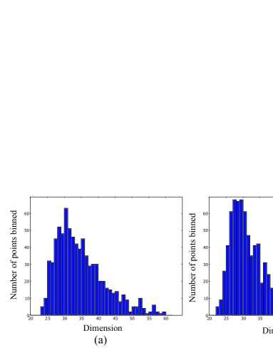
Figure 30: Histograms of maximum slopes $d_{x}^{1}$ using a unit bin width for a 54-dimensional rectangular solid (a) with equal side lengths, and (b) with 4 sides one fifth the length of the other 50. These show a concentration of slopes near $D/2=27$ and a long tail of relatively few binned points from the scatter plots in Figure 11.

We speculate that the process of generating postures in animal motion may be directly responsible for the presence of the flat regions in the $r$-$V$ curves and the associated clusters of closely-spaced points. We observe that typical hand motions for the tasks in this study consist of a sequence of somewhat discrete changes in individual finger positions or in coordinated groupings of fingers (e.g., flexing multiple fingers simultaneously), while other parts of the hand may remain stationary. Sampling from such motion may generate sequences of postures not unlike those generated by a random walk, where almost all sample paths have dimension $2$, independent of the dimension $(\geq 2)$ of the ambient space in which the walk takes place. We observed earlier that postures generated by random walks in our benchmark tests created localized subsets of closely-spaced points in the data, characterized by $r$-$V$ curves having regions that are almost flat. These flat regions were not observed when postures were uniformly sampled. We have not explored how long we would need to observe our robot before its observed random path would be expected to fill the six dimensional rectangular solid in joint space uniformly.

Our implementation of the PD-E algorithm is suitable for data sets of a few thousand points. The algorithm can analyze larger data sets than similar algorithms that calculate a complete matrix of interpoint distances for points in a data set. Our results were insensitive to the size of data sets in the range 1,000–8,000. However, experimental trials as long as possible are still necessary (for any method) to ensure that the sampling of postures from the robot or hand (a) approximate the full distribution of postures assumed in the specified task; and (b) are at a sufficiently low sampling rate to prevent close correlations between successive samples. The analysis summarized in Figure 22 showed that we required fewer data points than were collected in order to achieve robust results from PD-E .

We conclude from these tests that an algorithm such as the PD-E method presented here is effective in the qualitative exploration of complex geometric structure in motion capture data, and directly estimates bounds on the dimension of the set of postures assumed by an object in data space. Although this estimate is likely to be systematically biased toward an underestimate of the dimension we believe that it is feasible to correct this bias: these underestimates could be quantified by further empirical studies using benchmark data sets and their relationship to $D$ analyzed. Furthermore, the lack of differences between the estimated DOFs of the virtual and real robots suggest that we can expect improvement in the accuracy of dimension estimation for experimental data sets by continuing to refine our methods using abstract test data. In future work our method would be augmented by the parameterization of low-dimensional manifolds identified by nonlinear dimension estimation methods using PCA or more general techniques (e.g., kernel PCA [20]), which would elucidate finer detail in the geometric structure of the manifolds and their orientation in the whole data set.

4.2 Interpretation of Isomap results

The primary control parameters for Isomap are the neighbourhood size $K$ or the neighbourhood radius $\varepsilon$ and the number of coordinates used to represent a manifold. In the Swiss roll example there is a clear separation of spatial scales, and $\varepsilon$ is easily tuned to a scale much smaller than the separation of the folded layers of the manifold so that Isomap detects the one-dimensional nature of the curve rather than the globally three-dimensional nature of the whole set of points in the embedding space. However, in our motion capture data of a robot arm and a human hand there are no strongly separated spatial scales. The choice of appropriate values of $K$ or $\varepsilon$ for Isomap is more problematic in these cases, although PD-E analysis of the data sets can be used to predict good starting choices for these parameters. For instance, in the robot arm tests we obtained the best Isomap results with $\varepsilon=100$. In the PD-E analysis of the same data set we observed $\left[90,150\right]$ to be the approximate range of ball radii corresponding to points near the centre of the largest cluster in the scatter plot (Figure 24). Similarly, the characteristic number of points in those balls seem to provide good starting choices for the Isomap parameter $K$. For the robot arm this corresponds to $K\approx 50$.

4.3 Interpretation of PCA results

PCA is frequently used as a technique for dimension reduction, seeking to minimize the variance of residuals among projections of data in $\mathbb{R}^{D}$ onto a $d$-dimensional (linear) subspace. If this projection preserves relevant properties of the data set, then $d$ is regarded as an (upper) estimate for the dimension of the data set. Here we are primarily interested in methods that choose minimal values of $d$ that appear to preserve the geometric properties of the set, because these properties inform the process of modelling a biomechanical system as a dynamical system. The circumstances in which PCA works well to do this are ones in which the data is composed of a low dimensional signal and noise that is largely orthogonal to the subspace containing the signal. In these circumstances PCA will retain the signal while removing much of the noise from the data. It is hardly apparent that the underlying geometric structures produced by biomechanical systems have these properties, so we do not presume that PCA will be the most effective estimator of the DOFs of those systems.

PCA is commonly used to estimate dimension based on a fixed variance capture threshold $\tau$. However, the presence of nonlinear geometric structure in high-dimensional data sets means that the resulting estimates will be sensitive to noise or other small changes in the data if $\tau$ is not chosen to suit the properties of the data. Large values of $d$ occur when there are large numbers of small singular values. This implies that the cumulative norm of the first $k$ singular values changes slowly with $k$ as $k$ grows large, making the choice of $d$ highly dependent upon the choice of $\tau$.

The minimum value of $\tau$ needed to obtain a dimension estimate of $d$ for a data set with dimension $D\geq d$ is defined by the maximum possible value of $\sigma(d)$. This maximum is $\sqrt{d/D}$ for any $d$, and is obtained when all the singular values of the PCA decomposition are equal (for instance, in the case of a $D$-dimensional ball).

We find that graphing the PCA residuals $\rho(k)$ allows a definition of this threshold in terms of “knees” that appear to be better tuned to the properties of high dimensional data sets. In our exploration of synthetic and motion capture data sets we found that this method led to a more consistent and accurate upper estimate for the dimension of the data sets than by a priori selection of variance capture thresholds.

4.4 Significance for biomechanics

Biomechanical systems typically exhibit complex behaviour in their motion at multiple scales of time and space. As a result, the observable degrees of freedom expressed by the system can depend on the measurement scales chosen by the observer. As a prelude to developing dynamical models for the motion of a biomechanical system, we would like to characterize the number of “active” DOFs of the system to which the neuromuscular control has access. This number would be the most useful guide to the number of variables needed in a dynamical model. However, our measurements are complicated by the effects of instrumentation noise, and more importantly by “passive” DOFs of the system that are inherent in its mechanical properties—for instance, the elasticity of the skin surface on which we place reflective markers. In this paper we have begun to explore the effects on dimension estimation by systematic noise such as the passive properties of a skin-like barrier between the motion of a rigid body and the measurement instruments.

The measurement of the active DOFs is further complicated by the presence of correlations between observable variables, which we refer to as “synergies” [3]. The nervous system is involved with monitoring and controlling possibly many thousands of DOFs as part of its motor control functions. For this reason it is believed to utilize coordinated patterns of motor activity that act synergistically on multiple DOFs at once when performing different tasks, possibly taking advantage of basic biomechanical properties of the skeletomotor apparatus [21, 22]. Therefore, we expect the dynamics of neuromuscular control systems to be constrained to subsets of relatively low dimension when performing complex motions such as locomotion or manipulation.

Our analyses with PD-E and Isomap demonstrate the existence of low-dimensional nonlinear structures in constrained hand motions, such as those involving rhythmic motion retracing a closed curve in state space. In these cases PCA typically overestimates the DOFs involved because PCA is insensitive to nonlinear structure. This is apparent from the results for the synthetic test data sets consisting of the curve on a Swiss roll manifold and the union of a disc and a spiral embedded in a 5D ambient space. In the latter example, Isomap also fails to detect the one-dimensional nature of the spiral arms because the method is less sensitive to non-smooth data sets consisting of distinct subsets having different dimension.

Using PD-E we placed a conservative upper bound on the dimension of such constrained hand motions at roughly 10. However, we observed a high frequency of slopes in the range of 2–3 and 5–10 in the $r$-$V$ curves, estimates of 1–2 and 4–7 from PCA when detecting knees in the residuals, and estimates mostly in the range of 4–7 from Isomap. Thus, the combined estimates from the three methods we have focused on suggest that the neuromuscular control of hand motion involves a similar number of DOFs to that estimated by Santello et al. [1]. In that study the DOFs of hand motion were estimated in the context of a data set consisting of a wide range of static hand postures for grasping objects using two methods: PCA yielded an estimate of approximately 3 DOFs, and a combination of discrimant analysis and information theory estimated an upper bound of 5 or 6 DOFs. The quantitative comparison between the predictions of each method provide a less consistent picture of the differences between each task, but we plan to elucidate these comparisons further in future work that uses more subjects.

We noted the possible presence of multiple modes in the distributions of the slopes of $r$-$V$ curves for hand motion. This suggests that the underlying sets of postures in data space might not be smooth manifolds, and might instead be partitioned into subsets of different dimension. One hypothesis to explain this would be that hand motion involves motor subsystems expressing different numbers of DOFs depending on context. Testing this hypotheses will therefore require nonlinear methods such as those discussed here. We plan to systematically explore this possibility in future work, both in terms of the dimension of hand motion capture data and of corresponding electromyographic data from hand muscles.

References

- [1] M. Santello, M. Flanders, and J. F. Soechting, “Postural hand synergies for tool use,” Journal of Neuroscience, vol. 18, no. 23, pp. 10105–10115, 1998.
- [2] E. J. Weiss and M. Flanders, “Muscular and postural synergies of the human hand,” J. Neurophysiol., vol. 92, pp. 523–535, 2004.
- [3] A. d’Avella and E. Bizzi, “Shared and specific muscle synergies in natural motor behaviors,” Proc. Natl. Acad. Sci. USA, vol. 102, pp. 3076–3081, 2005.
- [4] A. B. Schwartz, D. M. Taylor, and S. I. Tillery, “Extraction algorithms for cortical control of arm prosthetics,” Curr. Opin. Neurobiol., vol. 11, no. 6, pp. 701–707, 2001.
- [5] K. M. Newell and D. E. Vaillancourt, “Dimensional change in motor learning,” Human Movement Science, vol. 20, pp. 695–715, 2001.
- [6] I. T. Jolliffe, Principal Component Analysis. Springer, 2nd ed., 2002.
- [7] J. B. Tenenbaum, V. de Silva, and J. C. Langford, “A global geometric framework for nonlinear dimensionality reduction,” Science, vol. 290, pp. 2319–2323, 2000.
- [8] T. Cox and M. Cox, Multidimensional scaling. London: Chapman & Hall, 1994.
- [9] S. T. Roweis and L. K. Saul, “Nonlinear dimensionality reduction by locally linear embedding,” Science, vol. 290, pp. 2323–2326, 2000.
- [10] M. Belkin and P. Niyogi, “Laplacian eigenmaps and spectral techniques for embedding and clustering,” in Advances in Neural Information Processing Systems 14, (Cambridge, MA), MIT Press, 2002.
- [11] D. L. Donoho and C. Grimes, “Hessian eigenmaps: New tools for nonlinear dimensionality reduction,” Proceedings of the National Academy of Science, pp. 5591–5596, 2003.
- [12] H. S. Greenside, A. Wolf, J. Swift, and T. Pignataro, “Impracticality of a box-counting algorithm for calculating dimensionality of strange attractors,” Phys. Rev. A, vol. 25, no. 6, pp. 3453–3456, 1983.
- [13] J. D. Farmer, E. Ott, and J. A. Yorke, “The dimension of chaotic attractors,” Physica D, vol. 7, pp. 153–180, 1983.
- [14] J. Guckenheimer, “Dimension estimates for attractors,” Contemporary Mathematics, vol. 28, pp. 357–367, 1984.
- [15] L.-S. Young, “Dimension, entropy and lyapunov exponents,” Ergod. Th. & Dynam. Sys., vol. 2, pp. 109–124, 1982.
- [16] L. Barreira, Y. Pesin, and J. Schmeling, “Dimension and product structure of hyperbolic measures,” Ann. of Math., vol. 149, no. 2, pp. 755–783, 1999.
- [17] M. Balasubramanian, E. L. Schwartz, J. B. Tenenbaum, V. de Silva, and J. C. Langford, “The isomap algorithm and topological stability,” Science, vol. 295, p. 7a, 2002.
- [18] T. C. Halsey, M. H. Jensen, L. P. Kadanoff, I. Procaccia, and B. I. Shraiman, “Fractal measures and their singularities: the characterization of strange sets,” Phys. Rev. A, vol. 33, pp. 1141–1151, 1986.
- [19] K. J. Falconer, Fractal geometry: Mathematical foundations and applications. Hoboken, NJ: John Wiley & Sons, Inc., 2 ed., 2003.
- [20] B. Scholkopf, A. Smola, and K.-R. Muller, “Nonlinear component analysis as a kernel eigenvalue problem,” Neural Computation, vol. 10, pp. 1299–1319, 1998.
- [21] M. C. Tresch, V. C. K. Cheung, and A. d’Avella, “Matrix factorization algorithms for the identification of muscle synergies: evaluation on simulated and experimental data sets,” Journal of Neurophysiology, vol. 95, pp. 2199–2212, 2006.
- [22] M. C. Tresch, P. Saltiel, A. d’Avella, and E. Bizzi, “Coordination and localization in spinal motor systems,” Brain Res. Review, pp. 66–79, 2002.