Second look at the spread of epidemics on networks

Abstract

In an important paper, M.E.J. Newman claimed that a general network-based stochastic Susceptible-Infectious-Removed (SIR) epidemic model is isomorphic to a bond percolation model, where the bonds are the edges of the contact network and the bond occupation probability is equal to the marginal probability of transmission from an infected node to a susceptible neighbor.  In this paper, we show that this isomorphism is incorrect and define a semi-directed random network we call the epidemic percolation network that is exactly isomorphic to the SIR epidemic model in any finite population.  In the limit of a large population, (i) the distribution of (self-limited) outbreak sizes is identical to the size distribution of (small) out-components, (ii) the epidemic threshold corresponds to the phase transition where a giant strongly-connected component appears, (iii) the probability of a large epidemic is equal to the probability that an initial infection occurs in the giant in-component, and (iv) the relative final size of an epidemic is equal to the proportion of the network contained in the giant out-component.  For the SIR model considered by Newman, we show that the epidemic percolation network predicts the same mean outbreak size below the epidemic threshold, the same epidemic threshold, and the same final size of an epidemic as the bond percolation model.  However, the bond percolation model fails to predict the correct outbreak size distribution and probability of an epidemic when there is a nondegenerate infectious period distribution.  We confirm our findings by comparing predictions from percolation networks and bond percolation models to the results of simulations.  In an appendix, we show that an isomorphism to an epidemic percolation network can be defined for any time-homogeneous stochastic SIR model.

1 Introduction

In an important paper, M. E. J. Newman studied a network-based Susceptible-Infectious-Removed (SIR) epidemic model in which infection is transmitted through a network of contacts between individuals [1].  The contact network itself is a random undirected network with an arbitrary degree distribution of the form studied by Newman, Strogatz, and Watts [2].  Given the degree distribution, these networks are maximally random, so they have no small loops and no degree correlations in the limit of a large population [2, 3, 4].

In the stochastic SIR model considered by Newman, the probability that an infected node $i$ makes infectious contact with a neighbor $j$ is given by $T_{ij}=1-\exp(-\beta_{ij}\tau_{i})$, where $\beta_{ij}$ is the rate of infectious contact from $i$ to $j$ and $\tau_{i}$ is the time that $i$ remains infectious.  (We use infectious contact to mean a contact that results in infection if and only if the recipient is susceptible.)  The infectious period $\tau_{i}$ is a random variable with the cumulative distribution function (cdf) $F(\tau)$, and the infectious contact rate $\beta_{ij}$ is a random variable with the cdf $F(\beta)$.  The infectious periods for all individuals are independent and identically distributed (iid), and the infectious contact rates for all ordered pairs of individuals are iid.

Under these assumptions, Newman claimed that the spread of disease on the contact network is exactly isomorphic to a bond percolation model on the contact network with bond occupation probability equal to the a priori probability of disease transmission between any two connected nodes in the contact network [1].  This probability is called the transmissibility and denoted by $T$:

$$T=\left\langle T_{ij}\right\rangle=\int_{0}^{\infty}\int_{0}^{\infty}(1-e^{-\beta_{ij}\tau_{i}})dF(\beta_{ij})dF(\tau_{i}).$$ (1)

Newman used this bond percolation model to derive the distribution of finite outbreak sizes, the critical transmissibility $T_{c}$ that defines the epidemic (i.e., percolation) threshold, and the probability and relative final size of an epidemic (i.e., an outbreak that never goes extinct).

As a counterexample, consider a contact network where each subject has exactly two contacts.  Assume that (i) $\tau_{i}=\tau_{0}>0$ with probability $p$ and $\tau_{i}=0$ with probability $1-p$ and (ii) $\beta_{ij}=\beta_{0}>0$ with probability one for all $ij$.  Under the SIR model, the probability that the infection of a randomly chosen node results in an outbreak of size one is $p_{1}=1-p+pe^{-2\beta_{0}\tau_{0}}$, which is the sum of the probability $1-p$ that $\tau=0$ and the probability $pe^{-2\beta_{0}\tau_{0}}$ that $\tau=\tau_{0}$ and disease is not transmitted to either contact.  Under the bond percolation model, the probability of a cluster of size one is $p_{1}^{bond}=(1-p+pe^{-\beta_{0}\tau_{0}})^{2}$, corresponding to the probability that neither of the bonds incident to the node are occupied.  Since

$$p_{1}-p_{1}^{bond}=p(1-p)(1-e^{-\beta_{0}\tau_{0}})^{2},$$

the bond percolation model correctly predicts the probability of an outbreak of size one only if $p=0$ or $p=1$.  When the infectious period is not constant, it underestimates this probability.  The supremum of the error is $0.25$, which occurs when $p=0.5$ and $\tau_{0}\rightarrow\infty$.  In this limit, the SIR model corresponds to a site percolation model rather than a bond percolation model.

When the distribution of infectious periods is nondegenerate, there is no bond occupation probability that will make the bond percolation model isomorphic to the SIR model.  To see why, suppose node $i$ has infectious period $\tau_{i}$ and degree $n_{i}$ in the contact network.  In the epidemic model, the conditional probability that $i$ transmits infection to a neighbor $j$ in the contact network given $\tau_{i}$ is

$$T_{\tau_{i}}=\int_{0}^{\infty}(1-e^{-\beta_{ij}\tau_{i}})dF(\beta_{ij}).$$ (2)

Since the contact rate pairs for all $n_{i}$ edges incident to $i$ are iid, the transmission events across these edges are (conditionally) independent Bernoulli($T_{\tau_{i}}$) random variables; but the transmission probabilities are strictly increasing in $\tau_{i}$, so the transmission events are (marginally) dependent unless $\tau_{i}=\tau_{0}$ with probability one for some fixed $\tau_{0}$.  In contrast, the bond percolation model treats the infections generated by node $i$ as $n_{i}$ (marginally) independent Bernoulli($T$) random variables regardless of the distribution of $\tau_{i}$.  Neither counterexample assumes anything about the global properties of the contact network, so Newman’s claim cannot be justified as an approximation in the limit of a large network with no small loops.

In Section 2, we define a semi-directed random network called the epidemic percolation network and show how it can be used to predict the outbreak size distribution, the epidemic threshold, and the probability and final size of an epidemic in the limit of a large population for any time-homogeneous SIR model.  In Section 3, we show that the network-based stochastic SIR model from [1] can be analyzed correctly using a semi-directed random network of the type studied by Boguñá and Serrano [3].  In Section 4, we show that it predicts the same epidemic threshold, mean outbreak size below the epidemic threshold, and relative final size of an epidemic as the bond percolation model.  In Section 5, we show that the bond percolation model fails to predict the distribution of outbreak sizes and the probability of an epidemic when the distribution of infectious periods is nondegenerate.  In Section 6, we compare predictions made by epidemic percolation networks and bond percolation models to the results of simulations.  In an appendix, we define epidemic percolation networks for a very general time-homogeneous stochastic SIR model and show that their out-components are isomorphic to the distribution of possible outcomes of the SIR model for any given set of imported infections.

2 Epidemic percolation networks

Consider a node $i$ with degree $n_{i}$ in the contact network and infectious period $\tau_{i}$.  In the SIR model defined above, the number of people who will transmit infection to $i$ if they become infectious has a binomial($n_{i},T$) distribution regardless of $\tau_{i}$.  If $i$ is infected along one of the $n_{i}$ edges, then the number of people to whom $i$ will transmit infection has a binomial($n_{i}-1,T_{\tau_{i}}$) distribution.  In order to produce the correct joint distribution of the number of people who will transmit infection to $i$ and the number of people to whom $i$ will transmit infection, we represent the former by directed edges that terminate at $i$ and the latter by directed edges that originate at $i$.  Since there can be at most one transmission of infection between any two persons, we replace pairs of directed edges between two nodes with a single undirected edge.

Starting from the contact network, a single realization of the epidemic percolation network can be generated as follows:

1. Choose a recovery period $\tau_{i}$ for every node $i$ in the network and choose a contact rate $\beta_{ij}$ for every ordered pair of connected nodes $i$ and $j$ in the contact network.

2. For each pair of connected nodes $i$ and $j$ in the contact network, convert the undirected edge between them to a directed edge from $i$ to $j$ with probability $(1-e^{-\beta_{ij}\tau_{i}})e^{-\beta_{ji}\tau_{j}}$, to a directed edge from $j$ to $i$ with probability $e^{-\beta_{ij}\tau_{i}}(1-e^{-\beta_{ji}\tau_{j}})$, and erase the edge completely with probability $e^{-\beta_{ij}\tau_{i}-\beta_{ji}\tau_{j}}$.  The edge remains undirected with probability $(1-e^{-\beta_{ij}\tau_{i}})(1-e^{-\beta_{ji}\tau_{j}})$.

The epidemic percolation network is a semi-directed random network that represents a single realization of the infectious contact process for each connected pair of nodes, so $4^{m}$ possible percolation networks exist for a contact network with $m$ edges.  The probability of each possible network is determined by the underlying SIR model.  The epidemic percolation network is very similar to the locally dependent random graph defined by Kuulasmaa [5] for an epidemic on a $d$-dimensional lattice.  There are two important differences: First, the underlying structure of the contact network is not assumed to be a lattice.  Second, we replace pairs of (occupied) directed edges between two nodes with a single undirected edge so that its component structure can be analyzed using a generating function formalism.

In the Appendix, we prove that the size distribution of outbreaks starting from any node in a time-homogeneous stochastic SIR model is identical to the distribution of its out-component sizes in the corresponding probability space of percolation networks.  Since this result applies to any time-homogeneous SIR model, it can be used to analyze network-based models, fully-mixed models (see [6]), and models with multiple levels of mixing.

2.1 Components of semi-directed networks

In this section, we briefly review the structure of directed and semi-directed networks as discussed in [3, 4, 7, 8].  In the next section, we relate this to the possible outcomes of an SIR model.

The indegree and outdegree of node $i$ are the number of incoming and outgoing directed edges incident to $i$.  Since each directed edge is an outgoing edge for one node and an incoming edge for another node, the mean indegree and outdegree are equal.  The undirected degree of node $i$ is the number of undirected edges incident to $i$.  The size of a component is the number of nodes it contains and its relative size is its size divided by the total size of the network.

The out-component of node $i$ includes $i$ and all nodes that can be reached from $i$ by following a series of edges in the proper direction (undirected edges are bidirectional).  The in-component of node $i$ includes $i$ and all nodes from which $i$ can be reached by following a series of edges in the proper direction.  By definition, node $i$ is in the in-component of node $j$ if and only if $j$ is in the out-component of $i$.  Therefore, the mean in- and out-component sizes in any (semi-)directed network are equal.

The strongly-connected component of a node $i$ is the intersection of its in- and out-components; it is the set of all nodes that can be reached from node $i$ and from which node $i$ can be reached.  All nodes in a strongly-connected component have the same in-component and the same out-component.  The weakly-connected component of node $i$ is the set of nodes that are connected to $i$ when the direction of the edges is ignored.

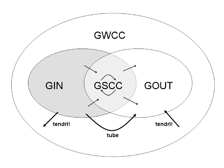
Figure 1: Schematic diagram of the giant components, tendrils, and tubes of a supercritical semi-directed network.  Adapted from Broder et al. [7] and Dorogovtsev et al. [8].

For giant components, we use the definitions given in [8, 9].  Giant components have asymptotically positive relative size in the limit of a large population.  All other components are “small” in the sense that they have asymptotically zero relative size.  There are two phase transitions in a semi-directed network: One where a unique giant weakly-connected component (GWCC) emerges and another where unique giant in-, out-, and strongly-connected components (GIN, GOUT, and GSCC) emerge.  The GWCC contains the other three giant components.  The GSCC is the intersection of the GIN and the GOUT, which are the common in- and out-components of nodes in the GSCC.  Tendrils are components in the GWCC that are outside the GIN and the GOUT.  Tubes are directed paths from the GIN to the GOUT that do not intersect the GSCC.  All tendrils and tubes are small components.  A schematic representation of these components is shown in Figure (1).

2.2 Epidemic percolation networks and epidemics

An outbreak begins when one or more nodes are infected from outside the population.  These are called imported infections.  The final size of an outbreak is the number of nodes that are infected before the end of transmission, and its relative final size is its final size divided by the total size of the network.  In the epidemic percolation network, the nodes infected in the outbreak can be identified with the nodes in the out-components of the imported infections.  This identification is made mathematically precise in the Appendix.

Informally, we define a self-limited outbreak to be an outbreak whose relative final size approaches zero in the limit of a large population and an epidemic to be an outbreak whose relative final size is positive in the limit of a large population.  There is a critical transmissibility $T_{c}$ that defines the epidemic threshold: The probability of an epidemic is zero when $T\leq T_{c}$, and the probability and final size of an epidemic are positive when $T>T_{c}$ [1, 10, 11, 12].

If all out-components in the epidemic percolation network are small, then only self-limited outbreaks are possible.  If the percolation network contains a GSCC, then any infection in the GIN will lead to the infection of the entire GOUT.  Therefore, the epidemic threshold corresponds to the emergence of the GSCC in the percolation network.  For any finite set of imported infections, the probability of an epidemic is equal to the probability that at least one imported infection occurs in the GIN.  The relative final size of an epidemic is equal to the proportion of the network contained in the GOUT.  Although some nodes outside the GOUT may be infected (e.g. nodes in tendrils and tubes), they constitute a finite number of small components whose total relative size is asymptotically zero.

3 Analysis of the SIR model

To analyze the SIR model from [1], we first calculate the probability generating function (pgf) of the degree distribution of the corresponding epidemic percolation network.  Then we use methods developed by Boguñá and Serrano [3] and Meyers et al. [4] to calculate the in- and out-component size distributions and the relative sizes of the GIN, GOUT, and GSCC.

3.1 Degree distribution

If $p_{n}$ is the probability that a node has degree $n$ in the contact network, then

$$\mathcal{G}(z)=\sum_{n=1}^{\infty}p_{n}z^{n}$$

is the probability generating function (pgf) for the degree distribution of the contact network.  If $p_{jkm}$ is the probability that a node in the epidemic percolation network has $j$ incoming edges, $k$ outgoing edges, and $m$ undirected edges, then

$$G(x,y,u)=\sum_{j=0}^{\infty}\sum_{k=0}^{\infty}\sum_{m=0}^{\infty}p_{jkm}x^{j}y^{k}u^{m}$$

is the pgf for the degree distribution of the percolation network.  Suppose nodes $i$ and $j$ are connected in the contact network with contact rates $(\beta_{ij},\beta_{ji})$ and infectious periods $\tau_{i}$ and $\tau_{j}$.  Let $g(x,y,u|\beta_{ij},\beta_{ji},\tau_{i},\tau_{j})$ be the conditional pgf for the number of incoming, outgoing, and undirected edges incident to $i$ that appear between $i$ and $j$ in the percolation network.  Then

$$g(x,y,u|\beta_{ij},\beta_{ji},\tau_{i},\tau_{j}) =e^{-\beta_{ij}\tau_{i}-\beta_{ji}\tau_{j}}+e^{-\beta_{ij}\tau_{i}}(1-e^{-\beta_{ji}\tau_{j}})x$$

$$+(1-e^{-\beta_{ij}\tau_{i}})e^{-\beta_{ji}\tau_{j}}y+(1-e^{-\beta_{ij}\tau_{i}})(1-e^{-\beta_{ji}\tau_{j}})u.$$

Given $\tau_{i}$, the conditional pgf for the number of incoming, outgoing, and undirected edges incident to $i$ that appear in the percolation network between $i$ and any neighbor of $i$ in the contact network is

$$g(x,y,u|\tau_{i}) =\int_{0}^{\infty}\int_{0}^{\infty}\int_{0}^{\infty}g(x,y,u|\beta_{ij},\beta_{ji},\tau_{i},\tau_{j})dF(\beta_{ij})dF(\beta_{ji})dF(\tau_{j})$$

$$=(1-T_{\tau_{i}})(1-T)+(1-T_{\tau_{i}})Tx+T_{\tau_{i}}(1-T)y+T_{\tau_{i}}Tu.$$ (3)

The pgf for the degree distribution of a node with infectious period $\tau_{i}$ is

$$G(x,y,u|\tau_{i})=\sum_{n=0}^{\infty}p_{n}(g(x,y,u|\tau_{i}))^{n}=\mathcal{G}(g(x,y,u|\tau_{i})).$$ (4)

Finally, the pgf for the degree distribution of the epidemic percolation network is

$$G(x,y,u)=\int_{0}^{\infty}G(x,y,u|\tau_{i})dF(\tau_{i}).$$ (5)

If $a$, $b$, and $c$ are nonnegative integers, let $G^{(a,b,c)}(x,y,u)$ be the derivative obtained after differentiating $a$ times with respect to $x$, $b$ times with respect to $y$, and $c$ times with respect to $u$.  Then the mean indegree and outdegree of the percolation network are

$$\left\langle k_{d}\right\rangle=G^{(1,0,0)}(1,1,1)=G^{(0,1,0)}(1,1,1)=T(1-T)\mathcal{G}^{\prime}(1),$$

and the mean undirected degree is

$$\left\langle k_{u}\right\rangle=G^{(0,0,1)}(1,1,1)=T^{2}\mathcal{G}^{\prime}(1).$$

3.2 Generating functions

When the contact network underlying an SIR epidemic model is an undirected random network with an arbitrary degree distribution, the pgf of its degree distribution can be used to calculate the distribution of small component sizes, the percolation threshold, and the relative sizes of the GIN, GOUT, and GSCC using methods developed by Boguñá and Serrano [3] and Meyers et al. [4].  These methods generalize earlier methods for undirected and purely directed networks [2, 1, 13, 14, 15, 16].  In this section, we review these results and introduce notation that will be used in the rest of the paper.  We discuss the case of networks with no two-point degree correlations, which is sufficient to analyze the SIR model from [1].

Let $G_{f}(x,y,u)$ be the pgf for the degree distribution of a node reached by going forward along a directed edge, excluding the edge used to reach the node.  Since the probability of reaching any node by following a directed edge is proportional to its indegree,

$$G_{f}(x,y,u)=\frac{1}{\left\langle k_{d}\right\rangle}\sum_{j,k,m}jp_{jkm}x^{j-1}y^{k}u^{m}=\frac{1}{\left\langle k_{d}\right\rangle}G^{(1,0,0)}(x,y,u).$$ (6)

Similarly, the pgf for the degree distribution of a node reached by going in reverse along a directed edge (excluding the edge used to reach the node) is

$$G_{r}(x,y,u)=\frac{1}{\left\langle k_{d}\right\rangle}G^{(0,1,0)}(x,y,u),$$ (7)

and the pgf for the degree distribution of a node reached by going to the end of an undirected edge (excluding the edge used to reach the node) is

$$G_{u}(x,y,u)=\frac{1}{\left\langle k_{u}\right\rangle}G^{(0,0,1)}(x,y,u).$$ (8)

3.2.1 Out-components

Let $H_{f}^{out}(z)$ be the pgf for the size of the out-component at the end of a directed edge and $H_{u}^{out}(z)$ be the pgf for the size of the out-component at the “end” of an undirected edge.  Then, in the limit of a large population,

$$H_{f}^{out}(z) =zG_{f}(1,H_{f}^{out}(z),H_{u}^{out}(z)),$$ (9a)

$$H_{u}^{out}(z) =zG_{u}(1,H_{f}^{out}(z),H_{u}^{out}(z)).$$ (9b)

The pgf for the out-component size of a randomly chosen node is

$$H^{out}(z)=zG(1,H_{f}^{out}(z),H_{u}^{out}(z)).$$ (10)

The probability that a node has a finite out-component in the limit of a large population is $H^{out}(1)$, so the probability that a randomly chosen node is in the GIN is $1-H^{out}(1)$.

The coefficients on $z^{0}$ in $H_{f}^{out}(z)$ and $H_{u}^{out}(z)$ are $G_{f}(1,0,0)$ and $G_{u}(1,0,0)$ respectively.  Therefore, power series for $H_{f}^{out}(z)$ and $H_{u}^{out}(z)$ can be computed to any desired order by iterating equations (9a) and (9b).  A power series for $H^{out}(z)$ can then be obtained using equation (10).  For any $z\in[0,1]$, $H_{f}^{out}(z)$ and $H_{u}^{out}(z)$ can be calculated with arbitrary precision by iterating equations (9a) and (9b) starting from initial values $y_{0},u_{0}\in[0,1)$.  Estimates of $H_{f}^{out}(z)$ and $H_{u}^{out}(z)$ can be used to estimate $H^{out}(z)$ with arbitrary precision.

The expected size of the out-component of a randomly chosen node below the epidemic threshold is $H^{out\prime}(1)$.  Taking derivatives in (10) yields

$$H^{out\prime}(1)=1+\left\langle k_{d}\right\rangle H_{f}^{out\prime}(1)+\left\langle k_{u}\right\rangle H_{u}^{out\prime}(1).$$ (11)

Taking derivatives in equations (9a) and (9b) and using the fact that $H_{f}^{out}(1)=H_{u}^{out}(1)=1$ below the epidemic threshold yields a set of linear equations for $H_{f}^{out\prime}(1)$ and $H_{u}^{out\prime}(1)$.  These can be solved to yield

$$H_{f}^{out\prime}(1)=\frac{1+G_{f}^{(0,0,1)}-G_{u}^{(0,0,1)}}{(1-G_{f}^{(0,1,0)})(1-G_{u}^{(0,0,1)})-G_{f}^{(0,0,1)}G_{u}^{(0,1,0)}}$$ (12)

and

$$H_{u}^{out\prime}(1)=\frac{1-G_{f}^{(0,1,0)}+G_{u}^{(0,1,0)}}{(1-G_{f}^{(0,1,0)})(1-G_{u}^{(0,0,1)})-G_{f}^{(0,0,1)}G_{u}^{(0,1,0)}},$$ (13)

where the argument of all derivatives is $(1,1,1)$.

3.2.2 In-components

The in-component size distribution of a semi-directed network can be derived using the same logic used to find the out-component size distribution, except that we consider going backwards along directed edges.  Let $H_{r}^{in}(z)$ be the pgf for the size of the in-component at the beginning of a directed edge, $H_{u}^{in}(z)$ be the pgf for the size of the in-component at the “beginning” of an undirected edge, and $H^{in}(z)$ be the pgf for the in-component size of a randomly chosen node.  Then, in the limit of a large population,

$$H_{r}^{in}(z) =zG_{r}(H_{r}^{in}(z),1,H_{u}^{in}(z)),$$ (14a)

$$H_{u}^{in}(z) =zG_{u}(H_{r}^{in}(z),1,H_{u}^{in}(z)),$$ (14b)

$$H^{in}(z) =zG(H_{r}^{in}(z),1,H_{u}^{in}(z)).$$ (14c)

The probability that a node has a finite in-component is $$H^{in}(1) 1-H^{in}(1) H^{in\prime}(1) H_{r}^{in}(z) H_{u}^{in}(z) H^{in}(z)$$, so the probability that a randomly chosen node is in the GOUT is .  The expected size of the in-component of a randomly chosen node is .  Power series and numerical estimates for , , and can be obtained by iterating these equations.

The expected size of the out-component of a randomly chosen node below the epidemic threshold is $H^{out\prime}(1)$.  Taking derivatives in equation (14c) yields

$$H^{in\prime}(1)=1+\left\langle k_{d}\right\rangle H_{r}^{in\prime}(1)+\left\langle k_{u}\right\rangle H_{u}^{in\prime}(1).$$ (15)

Taking derivatives in equations (14a) and (14b) and using the fact that $H_{r}^{in}(1)=H_{u}^{in}(1)=1$ in a subcritical network yields

$$H_{r}^{in\prime}(1)=\frac{1+G_{r}^{(0,0,1)}-G_{u}^{(0,0,1)}}{(1-G_{r}^{(1,0,0)})(1-G_{u}^{(0,0,1)})-G_{r}^{(0,0,1)}G_{u}^{(1,0,0)}}$$ (16)

and

$$H_{u}^{in\prime}(1)=\frac{1-G_{r}^{(1,0,0)}+G_{u}^{(1,0,0)}}{(1-G_{r}^{(1,0,0)})(1-G_{u}^{(0,0,1)})-G_{r}^{(0,0,1)}G_{u}^{(1,0,0)}},$$ (17)

where the argument of all derivatives is $(1,1,1)$.

3.2.3 Epidemic threshold

The epidemic threshold occurs when the expected size of the in- and out-components in the network becomes infinite.  This occurs when the denominators in equations (12) and (13) and equations (16) and (17) approach zero.  From the definitions of $G_{f}(x,y,u)$, $G_{r}(x,y,u)$ and $G_{u}(x,y,u)$, both conditions are equivalent to

$$(1-\frac{1}{\left\langle k_{d}\right\rangle}G^{(1,1,0)})(1-\frac{1}{\left\langle k_{u}\right\rangle}G^{(0,0,2)})-\frac{1}{\left\langle k_{d}\right\rangle\left\langle k_{u}\right\rangle}G^{(1,0,1)}G^{(0,1,1)}=0.$$

Therefore, there is a single epidemic threshold where the GSCC, the GIN, and the GOUT appear simultaneously in both purely directed networks [2, 1, 13, 14, 15, 16] and semi-directed networks [3, 4].

3.2.4 Giant strongly-connected component

A node is in the GSCC if its in- and out-components are both infinite.  A randomly chosen node has a finite in-component with probability $G(H_{r}^{in}(1),1,H_{u}^{in}(1))$ and a finite out-component with probability $G(1,H_{f}^{out}(1),H_{u}^{out}(1))$.  The probability that a node reached by following an undirected edge has finite in- and out-components is the solution to the equation

$$v=G_{u}(H_{r}^{in}(1),H_{f}^{out}(1),v),$$

and the probability that a randomly chosen node has finite in- and out-components is $G(H_{r}^{in}(1),H_{f}^{out}(1),v)$ [3].  Thus, the relative size of the GSCC is

$$1-G(H_{r}^{in}(1),1,H_{u}^{in}(1))-G(1,H_{f}^{out}(1),H_{u}^{out}(1))+G(H_{r}^{in}(1),H_{f}^{out}(1),v).$$

4 In-components

In this section, we prove that the in-component size distribution of the epidemic percolation network for the SIR model from [1] is identical to the component size distribution of the bond percolation model with bond occupation probability $T$.  The probability generating function for the total number of incoming and undirected edges incident to any node $i$ is

$$G(x,1,x|\tau_{i})=\mathcal{G}(g(x,1,x|\tau_{i}))=\mathcal{G}(1-T+Tx),$$

which is independent of $\tau_{i}$.  If node $i$ has degree $n_{i}$ in the contact network, then the number of nodes we can reach by going in reverse along a directed edge or an undirected edge has a binomial$(n_{i},T)$ distribution regardless of $\tau_{i}$.  If we reach node $i$ by going backwards along edges, the number of nodes we can reach from $i$ by continuing to go backwards (excluding the node from which we arrived) has a binomial$(n_{i}-1,T)$ distribution.  Therefore, the in-component of any node in the percolation network is exactly like a component of a bond percolation model with occupation probability $T$.  This argument was used to justify the mapping from an epidemic model to a bond percolation model in [1], but it does not apply to the out-components of the epidemic percolation network.

Methods of calculating the component size distribution of an undirected random network with an arbitrary degree distribution using the pgf of its degree distribution were developed by Newman et al. [2, 13, 14, 15, 16].  These methods were used to analyze the bond percolation model of disease transmission [1], obtaining results similar to those obtained by Andersson [17] for the epidemic threshold and the final size of an epidemic.  In this paragraph, we review these results and introduce notation that will be used in this section.  Let $\mathcal{G}(u)$ be the pgf for the degree distribution of the contact network.  Then the pgf for the degree of a node reached by following an edge (excluding the edge used to reach that node) is $\mathcal{G}_{1}(u)=\left\langle n\right\rangle^{-1}\mathcal{G}^{\prime}(u)$, where $\left\langle n\right\rangle=\mathcal{G}^{\prime}(1)$ is the mean degree of the contact network.  With bond occupation probability $T$, the number of occupied edges adjacent to a randomly chosen node has the pgf $\mathcal{G}(1-T+Tu)$ and the number of occupied edges from which infection can leave a node that has been infected along an edge has the pgf $\mathcal{G}_{1}(1-T+Tu)$.  The pgf for the size of the component at the end of an edge is

$$H_{1}(z)=z\mathcal{G}_{1}(1-T+TH_{1}(z))$$ (18)

and the pgf for the size of the component of a randomly chosen node is

$$H_{0}(z)=z\mathcal{G}(1-T+TH_{1}(z)).$$ (19)

The proportion of the network contained in the giant component is $1-H_{0}(1)$, and the mean size of components below the percolation threshold is $H_{0}^{\prime}(1)$.  $H_{0}(z)$ and $H_{1}(z)$ can be expanded as power series to any desired degree by iterating equations (18) and (19), and their value for any fixed $z\in[0,1]$ can be found by iteration from an initial value $z_{0}\in[0,1)$.

We can now prove that the distribution of component sizes in the bond percolation model is identical to the distribution of in-component sizes in the epidemic percolation network.

Lemma 1

$G_{r}(x,y,u)=G_{u}(x,y,u)$ for all $x,y,u.$

Proof. From equation (7),

$$G_{r}(x,y,u) =\frac{1}{T(1-T)\mathcal{G}^{\prime}(1)}G^{(0,1,0)}(x,y,u)$$

$$=\frac{1}{T\mathcal{G}^{\prime}(1)}\int_{0}^{\infty}\mathcal{G}^{\prime}(g(x,y,u|\tau_{i}))T_{\tau_{i}}dF(\tau_{i}).$$

From equation (8),

$$G_{u}(x,y,u) =\frac{1}{T^{2}\mathcal{G}^{\prime}(1)}G^{(0,0,1)}(x,y,u)$$

$$=\frac{1}{T\mathcal{G}^{\prime}(1)}\int_{0}^{\infty}\mathcal{G}^{\prime}(g(x,y,u|\tau_{i}))T_{\tau_{i}}dF(\tau_{i})\text{.}$$

Thus, the degree distribution of a node reached by going backwards along an edge is independent of whether it was a directed or undirected edge.    

Lemma 2

$H_{r}^{in}(z)=H_{u}^{in}(z)=H_{1}(z)$ for all $z$.

Proof. From equations (14a) and (14b),

$$H_{r}^{in}(z) =zG_{r}(H_{r}^{in}(z),1,H_{u}^{in}(z))$$

$$=zG_{u}(H_{r}^{in}(z),1,H_{u}^{in}(z))=H_{u}^{in}(z)\text{.}$$

Let $H_{\ast}^{in}(z)=H_{u}^{in}(z)=H_{r}^{in}(z)$.  Since $g(x,1,x|\tau_{i})=1-T+Tx$ for all $\tau_{i}$,

$$H_{\ast}^{in}(z) =\frac{z}{T\mathcal{G}^{\prime}(1)}\int_{0}^{\infty}\mathcal{G}^{\prime}(1-T+TH_{\ast}^{in}(z))T_{\tau_{i}}dF(\tau_{i})$$

$$=\frac{z}{\mathcal{G}^{\prime}(1)}\mathcal{G}^{\prime}(1-T+TH_{\ast}^{in}(z))\text{.}$$

From equation (18), we have

$$H_{1}(z)=\frac{z}{\mathcal{G}^{\prime}(1)}\mathcal{G}^{\prime}(1-T+TH_{1}^{in}(z))\text{.}$$

Since there is a unique pgf that solves this equation, $H_{\ast}^{in}(z)=H_{1}(z)$.  Thus, the in-component size distribution at the beginning of an edge is the same for directed and undirected edges, and it is identical to the distribution of component sizes at the end of an occupied edge in the bond percolation model.    

Theorem 3

$H^{in}(z)=H_{0}(z)$.

Proof. Let $H_{\ast}^{in}(z)=H_{r}^{in}(z)=H_{u}^{in}(z)$.  From equation (14c), the probability generating function for the distribution of in-component sizes in the percolation network is

$$H^{in}(z) =zG(H_{\ast}^{in}(z),1,H_{\ast}^{in}(z))$$

$$=z\int_{0}^{\infty}\mathcal{G}(g(H_{\ast}^{in}(z),1,H_{\ast}^{in}(z)|\tau_{i}))dF(\tau_{i})$$

$$=z\mathcal{G}(1-T+TH_{\ast}^{in}(z)).$$

When $H_{1}(z)$ is substituted for $H_{\ast}^{in}(z)$ (which is justified by the previous Lemma), this is identical to equation (19) for $H_{0}(z)$ in the bond percolation model.  Since there is a unique pgf solution to this equation, $H^{in}(z)=$ $H_{0}(z)$, so the distribution of in-components in the percolation network is identical to the distribution of component sizes in the bond percolation model.   

Since the mean size of out-components is equal to the mean size of in-components in any semi-directed network, the bond percolation model correctly predicts the mean size of outbreaks below the epidemic threshold.  Since the mean sizes of in- and out-components diverge simultaneously, the bond percolation model also correctly predicts the critical transmissibility $T_{c}$.  Since the probability of having a finite in-component in the percolation model is equal to the probability of being in a finite component of the bond percolation model, the bond percolation model also correctly predicts the final size of an epidemic.

5 Out-components

In this section, we prove that the distribution of out-component sizes in the epidemic percolation network for the SIR model from [1] is always different than the distribution of in-component sizes when there is a nondegenerate distribution of infectious periods.  As a corollary, we find that the probability of an epidemic in the SIR model from the Introduction is always less than or equal to its final size, with equality only when epidemics have probability zero or the infectious period is constant.  This is similar to a result obtained by Kuulasmaa and Zachary [18], who found that an SIR model defined on the $d$-dimensional integer lattice reduced to a bond percolation process if and only if the infectious period is constant.

The probability generating function for the total number of outgoing and undirected edges incident to a node $i$ with infectious period $\tau_{i}$ is

$$G(1,y,y|\tau_{i})=\mathcal{G}(g(1,y,y|\tau_{i}))=\mathcal{G}(1-T_{\tau_{i}}+T_{\tau_{i}}y),$$

where $T_{\tau_{i}}$ is the conditional probability of transmission across each edge given $\tau_{i}$, as defined in equation (2).  The number of nodes we can reach by going forwards along edges starting from $i$ has a Binomial($n_{i},T_{\tau_{i}}$) distribution.  If we reach a node $j$ by following an edge, then the number of nodes we can reach from $j$ by continuing to go forwards (excluding the node from which we arrived) has a binomial($k_{j}-1,T_{\tau_{j}}$) distribution.  Unless $\tau_{i}$ is constant, the out-components of the epidemic percolation network are not like the components of a bond percolation model.

Suppose $i$ and $j$ are connected in the contact network.  The conditional transmission probability from $j$ to $i$ given $\tau_{i}$ is always $T$.  Thus, an edge across which we leave any node is directed (i.e., outgoing) with probability $1-T$ and undirected with probability $T$.  This allows us to calculate the pgfs of the out-component distributions without differentiating between outgoing and undirected edges: Let

$$G_{o}(x,y,u) =(1-T)G_{f}(x,y,u)+TG_{u}(x,y,u)$$

$$=\frac{1}{\mathcal{G}^{\prime}(1)}\int_{0}^{\infty}\mathcal{G}^{\prime}(g(x,y,u|\tau_{i}))dF(\tau_{i})$$

be the probability generating function for the degree distribution of a node that we reach by going forward along an outgoing or undirected edge (excluding the edge along which we arrived).  Let

$$H_{\ast}^{out}(z)=(1-T)H_{f}^{out}(z)+TH_{u}^{out}(z)$$

be the probability generating function for the size of the out-component at the end of an outgoing or undirected edge.

Lemma 4

For the SIR model from [1],

$$H_{f}^{out}(z) =zG_{f}(1,H_{\ast}^{out}(z),H_{\ast}^{out}(z)),$$

$$H_{u}^{out}(z) =zG_{u}(1,H_{\ast}^{out}(z),H_{\ast}^{out}(z)),$$

$$H^{out}(z) =zG(1,H_{\ast}^{out}(z),H_{\ast}^{out}(z)),$$

and we have the following self-similarity equation:

$$H_{\ast}^{out}(z)=zG_{o}(1,H_{\ast}^{out}(z),H_{\ast}^{out}(z)).$$

Proof. From equation (3), we have

$$g(1,(1-T)y+Tu,(1-T)y+Tu|\tau_{i}) =1-T_{\tau_{i}}+T_{\tau_{i}}[(1-T)y+Tu]$$

$$=g(1,y,u|\tau_{i})$$

for all $y$, $u$, and $\tau_{i}$.  This allows us to rewrite equation (9a):

$$H_{f}^{out}(z) =zG_{f}(1,H_{f}^{out}(z),H_{u}^{out}(z))$$

$$=\frac{z}{(1-T)\mathcal{G}^{\prime}(1)}\int_{0}^{\infty}\mathcal{G}^{\prime}(g(1,H_{f}^{out}(z),H_{u}^{out}(z)|\tau_{i}))(1-T_{\tau_{i}})dF(\tau_{i})$$

$$=\frac{z}{(1-T)\mathcal{G}^{\prime}(1)}\int_{0}^{\infty}\mathcal{G}^{\prime}(g(1,H_{\ast}^{out}(z),H_{\ast}^{out}(z)|\tau_{i}))(1-T_{\tau_{i}})dF(\tau_{i})$$

$$=zG_{f}(1,H_{\ast}^{out}(z),H_{\ast}^{out}(z)).$$

Similarly, we can rewrite equation (9b):

$$H_{u}^{out}(z) =zG_{u}(1,H_{f}^{out}(z),H_{u}^{out}(z))$$

$$=\frac{z}{T\mathcal{G}^{\prime}(1)}\int_{0}^{\infty}\mathcal{G}^{\prime}(g(1,H_{f}^{out}(z),H_{u}^{out}(z)|\tau_{i}))T_{\tau_{i}}dF(\tau_{i})$$

$$=\frac{z}{T\mathcal{G}^{\prime}(1)}\int_{0}^{\infty}\mathcal{G}^{\prime}(g(1,H_{\ast}^{out}(z),H_{\ast}^{out}(z)|\tau_{i}))T_{\tau_{i}}dF(\tau_{i})$$

$$=zG_{u}(1,H_{\ast}^{out}(z),H_{\ast}^{out}(z)).$$

Finally, we can rewrite equation (10):

$$H^{out}(z) =zG(1,H_{f}^{out}(z),H_{u}^{out}(z))$$

$$=z\int_{0}^{\infty}\mathcal{G}(g(1,H_{f}^{out}(z),H_{u}^{out}(z)|\tau_{i}))dF(\tau_{i})$$

$$=z\int_{0}^{\infty}\mathcal{G}(g(1,H_{\ast}^{out}(z),H_{\ast}^{out}(z)|\tau_{i}))dF(\tau_{i})$$

$$=zG(1,H_{\ast}^{out}(z),H_{\ast}^{out}(z));$$

but then

$$H_{\ast}^{out}(z) =(1-T)H_{f}^{out}(z)+H_{u}^{out}(z)$$

$$=z[(1-T)G_{f}(1,H_{\ast}^{out}(z),H_{\ast}^{out}(z))+TG_{u}(1,H_{\ast}^{out}(z),H_{\ast}^{out}(z))]$$

$$=zG_{o}(1,H_{\ast}^{out}(z),H_{\ast}^{out}(z)).$$

As a corollary, we find that the analysis in Ref. [1] can be corrected if we let $G_{0}(x)=G(1,x,x)$ and $G_{1}(x)=G_{o}(1,x,x)$ (see equations (13) and (14) in [1]).    

Lemma 5

$H_{\ast}^{in}(z)\leq H_{\ast}^{out}(z)$ for all $z\in[0,1]$.

Proof. Since $\mathcal{G}^{\prime}$ is convex,

$$H_{\ast}^{out}(z) =zG_{o}(1,H_{\ast}^{out}(z),H_{\ast}^{out}(z))$$

$$=\frac{z}{\mathcal{G}^{\prime}(1)}\int_{0}^{\infty}\mathcal{G}^{\prime}(1-T_{\tau_{i}}+T_{\tau_{i}}H_{\ast}^{out}(z))dF(\tau_{i})$$

$$\geq\frac{z}{\mathcal{G}^{\prime}(1)}\mathcal{G}^{\prime}(1-T+TH_{\ast}^{out}(z))$$

by Jensen’s inequality.  Equality holds only if $z=0$, $H_{\ast}^{out}(z)=1$, $\mathcal{G}^{\prime}$ is constant, or $\tau_{i}$ is constant.  Since $H_{\ast}^{in}(z)$ is the solution to

$$H_{\ast}^{in}(z)=\frac{z}{\mathcal{G}^{\prime}(1)}\mathcal{G}^{\prime}(1-T+TH_{\ast}^{in}(z))\text{,}$$

we must have $H_{\ast}^{out}(z)\geq H_{\ast}^{in}(z)$.  This can be seen by fixing $z$ and considering the graphs of $y=zG_{o}(1,x,x)$ and $y=\frac{z}{\mathcal{G}^{\prime}(1)}\mathcal{G}^{\prime}(1-T+Tx)$.  $H_{\ast}^{out}(z)$ is the value of $x$ at which $y=zG_{o}(1,x,x)$ intersects the line $y=x$.  $H_{\ast}^{in}(z)$ is the value of $x$ at which $y=\frac{z}{\mathcal{G}^{\prime}(1)}\mathcal{G}^{\prime}(1-T+Tx)$ intersects the line $y=x$.  Since $zG_{o}(1,x,x)\geq\frac{z}{\mathcal{G}^{\prime}(1)}\mathcal{G}^{\prime}(1-T+Tx)$, we must have $H_{\ast}^{out}(z)\geq H_{\ast}^{in}(z)$.    

Theorem 6

$H^{in}(z)\leq H^{out}(z)$ for all $z\in[0,1]$.  Equality holds only when $z=0$, $z=1$ and the percolation network is subcritical, or the infectious period is constant.

Proof. From equation (14c),

$$H^{in}(z) =zG(H_{\ast}^{in}(z),1,H_{\ast}^{in}(z))$$

$$=z\mathcal{G}(1-T+TH_{\ast}^{in}(z))\text{.}$$

From equation (10),

$$H^{out}(z) =zG(1,H_{\ast}^{out}(z),H_{\ast}^{out}(z))$$

$$=z\int_{0}^{\infty}\mathcal{G}(1-T_{\tau_{i}}+T_{\tau_{i}}H_{\ast}^{out}(z))dF(\tau_{i})$$

$$\geq z\mathcal{G}(1-T+TH_{\ast}^{out}(z))$$

$$\geq z\mathcal{G}(1-T+TH_{\ast}^{in}(z))\text{.}$$

The first inequality follows from the convexity of $\mathcal{G}$ and Jensen’s inequality.  The second follows from the fact that $\mathcal{G}$ is nondecreasing and $H_{\ast}^{out}(z)\geq H_{\ast}^{in}(z)$.  Equality holds in both inequalities only if $z=0$, $\mathcal{G}$ is constant, $H_{\ast}^{in}(z)=1$, or $\tau_{i}$ is constant.    

Since the probability of an epidemic is $1-H^{out}(1)$ and the final size of an epidemic is $1-H^{in}(1)$, it follows that the probability of an epidemic is always less than or equal to its final size in the SIR model from [1].  When the infectious period is constant, $H^{out}(z)=H^{in}(z)$ for all $z\in[0,1]$, so the in- and out-component size distributions are identical and the probability and final size of an epidemic are equal.  When the infectious period has a nondegenerate distribution and the percolation network is subcritical, $H^{out}(z)>H^{in}(z)$ for all $z\in(0,1)$ (so the in- and out-components have dissimilar size distributions) but $H^{out}(1)=H^{in}(1)=1$ (so the probability and final size of an epidemic are both zero).  If the network is supercritical and the infectious period is nonconstant, $H^{out}(z)>H^{in}(z)$ for all $z\in[0,1]$, so in- and out-components have dissimilar size distributions and the probability of an epidemic is strictly less than its final size.

Since the bond percolation model predicts the distribution of in-component sizes, it cannot predict the distribution of out-component sizes or the probability of an epidemic for any SIR model with a nonconstant infectious period.  However, it does establish an upper limit for the probability of an epidemic in an SIR model.  We have recently become aware of independent work [19] that shows similar results for more general sources of variation in infectiousness and susceptibility in a model where these are independent and uses Jensen’s inequality to establish a lower bound for the probability and final size of an epidemic.  The lower bound corresponds to a site percolation model with site occupation probability $T$, which is the model that minimized the probability of no transmission in the Introduction.

6 Simulations

In a series of simulations, the bond percolation model correctly predicted the mean outbreak size (below the epidemic threshold), the epidemic threshold, and the final size of an epidemic [1].  In Section 4, we showed that the epidemic percolation network generates the same predictions for these quantities.

In Newman’s simulations, the contact network had a power-law degree distribution with an exponential cutoff around degree $\kappa$, so the probability that a node has degree $k$ is proportional to $k^{-\alpha}e^{-1/\kappa}$ for all $k\geq 1$.  This distribution was chosen to reflect degree distributions observed in real-world networks [1, 13, 14, 15].  The probability generating function for this degree distribution is

$$\mathcal{G}(z)=\frac{\operatorname{Li}_{\alpha}(ze^{-1/\kappa})}{\operatorname{Li}_{\alpha}(e^{-1/\kappa})},$$

where $\operatorname{Li}_{\alpha}(z)$ is the $\alpha$-polylogarithm of $z$.  In [1], Newman used $\alpha=2$.

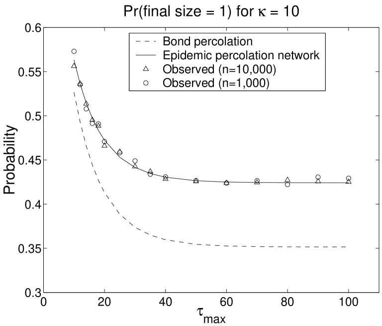
Figure 2: The predicted and observed probabilities of an outbreak of size one on a contact network with $\kappa=10$ as a function of $\tau_{\max}$.  Models were run for $\tau_{\max}=10$, $12$, $14$, $16$, $18$, $20$, $25$, $30$, $35$, $40$, $50$, $60$, $70$, $80$, $90$, $100$.  Each observed value is based on $10,000$ simulations in a population of size $n$.  For $n=10,000$, $1,000$ simulations were conducted on each of $10$ contact networks.  For $n=1,000$, $100$ simulations were conducted on each of $100$ contact networks.  

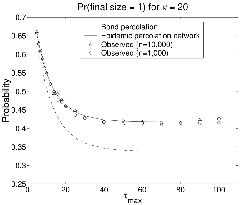
Figure 3: The predicted and observed probabilities of an outbreak of size one on a contact network with $\kappa=20$ as a function of $\tau_{\max}$.  Models were run for $\tau_{\max}=5$, $6$, $7$, $8$, $9$, $10$, $12$, $14$, $16$, $18$, $20$, $25$, $30$, $40$, $50$, $60$, $70$, $80$, $90$, and $100$.  Each observed value is based on $10,000$ simulations in a population of size $n$.  For $n=10,000$, $1000$ simulations were conducted on each of ten contact networks.  For $n=1000$, $100$ simulations were conducted on each of $100$ contact networks.  

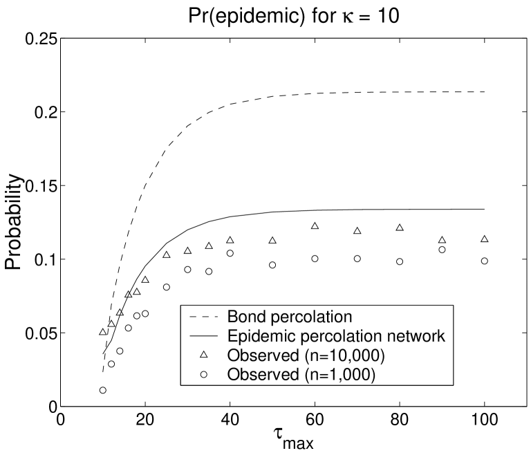
Figure 4: The predicted and observed probabilities of an epidemic on a contact network with $\kappa=10$ as a function of $\tau_{\max}$.  Models were run for $\tau_{\max}=10$, $12$, $14$, $16$, $18$, $20$, $25$, $30$, $35$, $40$, $50$, $60$, $70$, $80$, $90$, and $100$.  Each observed value is based on $10,000$ simulations in a population of size $n$.  For $n=10,000$, $1000$ simulations were conducted on each of ten contact networks.  For $n=1000$, $100$ simulations were conducted on each of $100$ contact networks.  

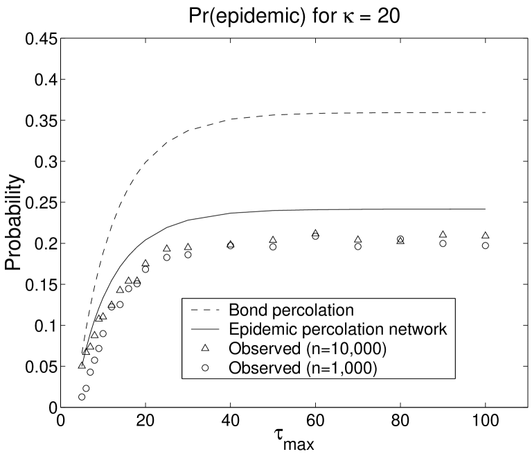
Figure 5: The predicted and observed probabilities of an epidemic on a contact network with $\kappa=20$ as a function of $\tau_{\max}$.  Models were run for $\tau_{\max}=5$, $6$, $7$, $8$, $9$, $10$, $12$, $14$, $16$, $18$, $20$, $25$, $30$, $40$, $50$, $60$, $70$, $80$, $90$, and $100$.  Each observed value is based on $10,000$ simulations in a population of size $n$.  For $n=10,000$, $1000$ simulations were conducted on each of ten contact networks.  For $n=1000$, $100$ simulations were conducted on each of $100$ contact networks.

In our simulations, we retained the same contact network but used a contact model adapted from the counterexample in the Introduction.  We fixed $\beta_{ij}=\beta_{0}=0.1$ for all $ij$ and let $\tau_{i}=1$ with probability $0.5$ and $\tau_{i}=\tau_{\max}>1$ with probability $0.5$ for all $i$.  The predicted probability of an outbreak of size one is $G(1,0,0)$ in the epidemic percolation network and $G(0,1,0)$ in the bond percolation model.  The predicted probability of an epidemic is $1-H^{out}(1)$ in the epidemic percolation network and $1-H^{in}(1)$ in the bond percolation model.  In all simulations, an epidemic was declared when at least $100$ persons were infected (this low cutoff produces a slight overestimate of the probability of an epidemic in the simulations, favoring the bond percolation model).  Figures 2 and 3 show that percolation networks accurately predicted the probability of an outbreak of size one for all $(n,\kappa,\tau_{\max})$ combinations, whereas the bond percolation model consistently underestimated these probabilities.  Figures 4 and 5 show that the bond percolation model significantly overestimated the probability of an epidemic for all $(n,\kappa,\tau_{\max})$ combinations.  The percolation network predictions were far closer to the observed values.

7 Discussion

For any time-homogeneous SIR epidemic model, the problem of analyzing its final outcomes can be reduced to the problem of analyzing the components of an epidemic percolation network.  The distribution of outbreak sizes starting from a node $i$ is identical to the distribution of its out-component sizes in the probability space of percolation networks.  Calculating this distribution may be extremely difficult for a finite population, but it simplifies enormously in the limit of a large population for many SIR models.  For a single randomly chosen imported infection in the limit of a large population, the distribution of self-limited outbreak sizes is equal to the distribution of small out-component sizes and the probability of an epidemic is equal to the relative size of the GIN.  For any finite set of imported infections, the relative final size of an epidemic is equal to the relative size of the GOUT.

In this paper, we used epidemic percolation networks to reanalyze the SIR epidemic model studied in [1].  The mapping to a bond percolation model correctly predicts the distribution of in-component sizes, the critical transmissibility, and the final size of an epidemic.  However, it fails to predict the correct distribution of outbreak sizes and overestimates the probability of an epidemic when the infectious period is nonconstant.  Since all known infectious diseases have nonconstant infectious periods and heterogeneity in infectiousness has important consequences in real epidemics [21, 20, 22], it is important to be able to analyze such models correctly.

The exact finite-population isomorphism between a time-homogeneous SIR model and our semi-directed epidemic percolation network is not only useful because it provides a rigorous foundation for the application of percolation methods to a large class of SIR epidemic models (including fully-mixed models as well as network-based models), but also because it provides further insight into the epidemic model.  For example, we used the mapping to an epidemic percolation network to show that the distribution of in- and out-component sizes in the SIR model from [1] could be calculated by treating the incoming and outgoing infectious contact processes as separate directed percolation processes, as in [19].  However, in contrast with [19], the semi-directed epidemic percolation network isolates the fundamental role of the GSCC in the emergence of epidemics.  The design of interventions to reduce the probability and final size of an epidemic is a central concern of infectious disease epidemiology.  In a forthcoming paper, we analyze both fully-mixed and network-based SIR models in which vaccinating those nodes most likely to be in the GSCC is shown to be the most effective strategy for reducing both the probability and final size of an epidemic.  If the incoming and outgoing contact processes are treated separately, the notion of the GSCC is lost.

Acknowledgments: This work was supported by the US National Institutes of Health cooperative agreement 5U01GM076497 “Models of Infectious Disease Agent Study” (E.K.) and Ruth L. Kirchstein National Research Service Award 5T32AI007535 “Epidemiology of Infectious Diseases and Biodefense” (E.K.), as well as a research grant from the Institute for Quantitative Social Sciences at Harvard University (E.K.).  Joel C. Miller’s comments on the proofs in Sections 3 and 4 were extremely valuable, and we are also grateful for the comments of Marc Lipsitch, James H. Maguire, and the anonymous referees of PRE.  E.K. would also like to thank Charles Larson and Stephen P. Luby of the Health Systems and Infectious Diseases Division at ICDDR,B (Dhaka, Bangladesh).

Appendix A Epidemic percolation networks

It is possible to define epidemic percolation networks for a much larger class of stochastic SIR epidemic models than the one from [1].  First, we specify an SIR model using probability distributions for recovery periods in individuals and times from infection to infectious contact in ordered pairs of individuals.  Second, we outline time-homogeneity assumptions under which the epidemic percolation network is well-defined.  Finally, we define infection networks and use them to show that the final outcome of the SIR model depends only on the set of imported infections and the epidemic percolation network.

A.1 Model specification

Suppose there is a closed population in which every susceptible person is assigned an index $i\in\{1,...,n\}$.  A susceptible person is infected upon infectious contact, and infection leads to recovery with immunity or death.  Each person $i$ is infected at his or her infection time $t_{i}$, with $t_{i}=\infty$ if $i$ is never infected.  Person $i$ is removed (i.e., recovers from infectiousness or dies) at time $t_{i}+r_{i}$, where the recovery period $r_{i}$ is a random sample from a probability distribution $f_{i}(r)$.  The recovery period $r_{i}$ may be the sum of a latent period, when $i$ is infected but not yet infectious, and an infectious period, when $i$ can transmit infection.  We assume that all infected persons have a finite recovery period.  Let $S(t)=\{i:t_{i}>t\}$ be the set of susceptible individuals at time $t$.  Let $t_{(1)}\leq t_{(2)}\leq...\leq t_{(n)}$ be the order statistics of $t_{1},...,t_{n}$, and let $i_{(k)}$ be the index of the $k^{\text{th}}$ person infected.

When person $i$ is infected, he or she makes infectious contact with person $j\neq i$ after an infectious contact interval $\tau_{ij}$.  Each $\tau_{ij}$ is a random sample from a conditional probability density $f_{ij}(\tau|r_{i})$.  Let $\tau_{ij}=\infty$ if person $i$ never makes infectious contact with person $j$, so $f_{ij}(\tau|r_{i})$ has a probability mass concentrated at infinity.  Person $i$ cannot transmit disease before being infected or after recovering, so $f_{ij}(\tau|r_{i})=0$ for all $\tau<0$ and all $\tau\in[r_{i},\infty)$.   The infectious contact time $t_{ij}=t_{i}+\tau_{ij}$ is the time at which person $i$ makes infectious contact with person $j$.  If person $j$ is susceptible at time $t_{ij}$, then $i$ infects $j$ and $t_{j}=t_{ij}$.  If $t_{ij}<\infty$, then $t_{j}\leq t_{ij}$ because person $j$ avoids infection at $t_{ij}$ only if he or she has already been infected.

For each person $i$, let his or her importation time $t_{0i}$ be the first time at which he or she experiences infectious contact from outside the population, with $t_{0i}=\infty$ if this never occurs.  Let $F_{0}(\mathbf{t}_{0})$ be the cumulative distribution function of the importation time vector $\mathbf{t}_{0}=(t_{01},t_{02},...,t_{0n})$.

A.2 Epidemic algorithm

First, an importation time vector $\mathbf{t}_{0}$ is chosen.  The epidemic begins with the introduction of infection at time $t_{(1)}=\min_{i}(t_{0i})$.  Person $i_{(1)}$ is assigned a recovery period $r_{i_{(1)}}$.  Every person $j\in S(t_{(1)})$ is assigned an infectious contact time $t_{i_{(1)}j}=t_{(1)}+\tau_{i_{(1)}j}$.  We assume that there are no tied infectious contact times less than infinity.  The second infection occurs at $t_{(2)}=\min_{j\in S(t_{(1)})}\min(t_{0j},t_{i_{(1)}j})$, which is the time of the first infectious contact after person $i_{(1)}$ is infected.  Person $i_{(2)}$ is assigned a recovery period $r_{i_{(2)}}$.  After the second infection, each of the remaining susceptibles is assigned an infectious contact time $t_{i_{(2)}j}=t_{(2)}+\tau_{i_{(2)}j}$.  The third infection occurs at $t_{(3)}=\min_{j\in S(t_{(2)})}\min(t_{0j},t_{i_{(1)}j},t_{i_{(2)}j})$, and so on.  After $k$ infections, the next infection occurs at $t_{(k+1)}=\min_{j\in S(t_{(k)})}\min(t_{0j},t_{i_{(1)}j},...,t_{i_{(k)}j})$.  The epidemic stops after $m$ infections if and only if $t_{(m+1)}=\infty$.

A.3 Time homogeneity assumptions

In principle, the above epidemic algorithm could allow the infectious period and outgoing infectious contact intervals for individual $i$ to depend on all information about the epidemic available up to time $t_{i}$.  In order to generate an epidemic percolation network, we must ensure that the joint distributions of recovery periods and infectious contact intervals are defined a priori.  The following restrictions are sufficient:

1. We assume that the distribution of the recovery period vector $\mathbf{r}=(r_{1},r_{2},...,r_{n})$ does not depend on the importation time vector $\mathbf{t}_{0}$, the contact interval matrix $\mathbf{\tau}=[\tau_{ij}]$, or the history of the epidemic.

2. We assume that the distribution of the infectious contact interval matrix $\mathbf{\tau}$ does not depend on $\mathbf{t}_{0}$ or the history of the epidemic.

With these time-homogeneity assumptions, the cumulative distributions functions $F(\mathbf{r})$ of recovery periods and $F(\mathbf{\tau}|\mathbf{r})$ of infectious contact intervals are completely specified a priori.  Given$\ \mathbf{r}$ and $\mathbf{\tau}$, the epidemic percolation network is a semi-directed network in which there is a directed edge from $i$ to $j$ iff $\tau_{ij}<\infty$ and $\tau_{ji}=\infty$, a directed edge from $j$ to $i$ iff $\tau_{ij}=\infty$ and $\tau_{ji}<\infty$, and an undirected edge between $i$ and $j$ iff $\tau_{ij}<\infty$ and $\tau_{ji}<\infty$.  The entire time course of the epidemic is determined by $\mathbf{r}$, $\mathbf{\tau}$, and $\mathbf{t}_{0}$.  However, its final size depends only on the set $\{i:t_{0i}<\infty\}$ of possible imported infections and the epidemic percolation network corresponding to $\mathbf{\tau}$.  In order to prove this, we first define the infection network, which records the chain of infection from a single realization of the epidemic model.

A.4 Infection networks

Let $v_{i}$ be the index of the person who infected person $i$, with $v_{i}=0$ for imported infections and $v_{i}=\infty$ for uninfected nodes.  If tied finite infectious contact times are possible, then choose $v_{i}$ from all $j$ such that $t_{ji}=t_{i}$.  The infection network has the edge set $\{v_{i}i:0<v_{i}<\infty\}$.  It is a purely directed subgraph of the epidemic percolation network corresponding to $\mathbf{\tau}$ because $\tau_{v_{i}i}<\infty$ for every edge $v_{i}i$.  Since each node has at most one incoming edge, all components of the infection network are trees or isolated nodes.  Every imported case is either the root node of a tree or an isolated node.  Every person infected through transmission within the population is a nonroot node in a tree.  Uninfected persons are isolated nodes.

The infection network can be represented by a vector $\mathbf{v}=(v_{1},..,v_{n})$, as in Ref. [23].  If $v_{j}=0$, then $t_{j}=t_{0j}$.  If $0<v_{j}<\infty$, then $j$ is in a component of the infection network with a root node $imp_{j}$ and its infection time is

$$t_{j}=t_{imp_{j}}+\sum_{k=1}^{m}\tau_{i_{k}j_{k}},$$

where the edges $i_{1}j_{1},...,i_{m}j_{m}$ form a directed path from $imp_{j}$ to $j$.  This path is unique because all nontrivial components of the infection network are trees.  If $v_{j}=\infty$, then $t_{j}=\infty$.  The removal time of each node $i$ is $t_{i}+r_{i}$.  If there is more than one possible infection network, they must all be consistent with $(t_{1},...,t_{n})$ by definition of $v_{i}$.  Therefore, the entire time course of the epidemic is determined by the importation time vector $\mathbf{t}_{0}$, the recovery period vector $\mathbf{r}$, and the infectious contact interval matrix $\mathbf{\tau}$.

A.5 Final outcomes and epidemic percolation networks

Theorem 7

In an epidemic with infectious contact interval matrix $\mathbf{\tau}$, a node is infected if and only if it is in the out-component of a node $i$ with $t_{0i}<\infty$ in the percolation network.  (Equivalently, a node is infected if and only if its in-component includes a node $i$ with $t_{0i}<\infty$.)  Therefore, the final outcome of the SIR model depends only on the set of imported infections and the epidemic percolation network corresponding to $\mathbf{\tau}$.

Proof. Suppose that person $j$ is in the out-component of a node $i$ with $t_{0i}<\infty$ in the epidemic percolation network corresponding to $\mathbf{\tau}$.  Then there is a sequence $i_{1}j_{1},...,i_{m}j_{m}$ such that $i_{1}=i$, $j_{m}=j$, and $\tau_{i_{k}j_{k}}<\infty$ for $1\leq k\leq m$, so

$$t_{j}\leq t_{0i}+\sum_{k=1}^{m}\tau_{i_{k}j_{k}}<\infty,$$

and $j$ must be infected during the epidemic.  Now suppose that $t_{j}<\infty$.  Then there exists an imported case $i$ and a sequence $i_{1}j_{1},...,i_{m}j_{m}$ such that $i_{1}=i$, $j_{m}=j$, and

$$t_{j}=t_{i}+\sum_{k=1}^{m}\tau_{i_{k}j_{k}}.$$

Since $t_{j}<\infty$, it follows that $\tau_{i_{k}j_{k}}<\infty$ for all $k$.  But then the epidemic percolation network corresponding to $\mathbf{\tau}$ has an edge with the proper direction or an undirected edge between $i_{k}$ and $j_{k}$ for all $k$, so $j$ is in the out-component of $i$.     

By the law of iterated expectation (conditioning on $\mathbf{\tau})$, this result implies that the distribution of outbreak sizes caused by the introduction of infection to node $i$ is identical to the distribution of his or her out-component sizes in the probability space of epidemic percolation networks.  Furthermore, the probability that person $i$ gets infected in an epidemic is equal to the probability that his or her in-component contains at least one imported infection.  This isomorphism holds in any finite population.  In the limit of a large population, the probability that node $i$ is infected in an epidemic is equal to the probability that he or she is in the GOUT and the probability that an epidemic results from the infection of node $i$ is equal to the probability that he or she is in the GIN.  This logic can be extended to predict the mean size of self-limited outbreaks and the probability and final size of an epidemic for outbreaks started by any given set of imported infections.

Appendix B Figures and tables

References

- [1] M. E. J. Newman (2002). Spread of epidemic disease on networks. Physical Review E 66, 016128.
- [2] M. E. J. Newman, S. H. Strogatz, and D. J. Watts (2001). Random graphs with arbitrary degree distributions and their applications, Physical Review E 64, 026118.
- [3] M. Boguñá and M. A. Serrano (2005). Generalized percolation in random directed networks. Physical Review E 72, 016106.
- [4] L. A. Meyers, M. E. J. Newman, and B. Pourbohloul (2006). Predicting epidemics on directed contact networks. Journal of Theoretical Biology 240(3): 400-418.
- [5] K. Kuulasmaa (1982). The spatial general epidemic and locally dependent random graphs. Journal of Applied Probability 19(4): 745-758.
- [6] E. Kenah and J. Robins (2007). Network-based analysis of stochastic SIR epidemic models with random and proportionate mixing. arXiv: q-bio.QM/0702027.
- [7] A. Broder, R. Kumar, F. Maghoul, P. Raghavan, S. Rajagopalan, R. Stata, A. Tomkins, and J. Weiner (2000). Graph structure in the Web. Computer Networks 33: 309-320.
- [8] S.N. Dorogovtsev, J.F.F. Mendes, and A.N. Sakhunin (2001). Giant strongly connected component of directed networks. Physical Review E, 64: 025101(R).
- [9] N. Schwartz, R. Cohen, D. ben-Avraham, A.-L. Barabási, and S. Havlin (2002). Percolation in directed scale-free networks. Physical Review E 66, 015104(R).
- [10] H. Andersson and T. Britton (2000). Stochastic Epidemic Models and Their Statistical Analysis (Lecture Notes in Statistics v.151). New York: Springer-Verlag.
- [11] O. Diekmann and J. A. P. Heesterbeek (2000). Mathematical Epidemiology of Infectious Diseases: Model Building, Analysis and Interpretation. Chichester (UK): John Wiley & Sons.
- [12] L. M. Sander, C. P. Warren, I. M. Sokolov, C. Simon, and J. Koopman (2002). Percolation on heterogeneous networks as a model for epidemics. Mathematical Biosciences 180, 293-305.
- [13] R. Albert and A-L. Barabási (2002). Statistical mechanics of complex networks. Reviews of Modern Physics, 74: 47-97.
- [14] M. E. J. Newman (2003). The structure and function of complex networks. SIAM Reviews, 45(2): 167-256.
- [15] M. E. J. Newman (2003). Random graphs as models of networks, in Handbook of Graphs and Networks, pp. 35-68. S. Bornholdt and H. G. Schuster, eds. Berlin: Wiley-VCH, 2003.
- [16] M.E.J. Newman, A.-L. Barabási, and D.J. Watts (2006). The Structure and Dynamics of Networks (Princeton Studies in Complexity). Princeton: Princeton University Press.
- [17] H. Andersson. Limit theorems for a random graph epidemic model (1998). The Annals of Applied Probability 8(4): 1331-1349.
- [18] K. Kuulasmaa and S. Zachary (1984). On spatial general epidemics and bond percolation processes. Journal of Applied Probability 21(4): 911-914.
- [19] J. Miller (2007). Predicting the size and probability of epidemics in populations with heterogeneous infectiousness and susceptibility. Physical Review E 76: 010101(R).
- [20] M. Lipsitch, T. Cohen, B. Cooper, J. M. Robins, S. Ma, L. James, G. Gopalakrishna, S. K. Chew, C. C. Tan, M. H. Samore, D. Fishman, and M. Murray (2003). Transmission dynamics and control of Severe Acute Respiratory Syndrome. Science 300: 1966-1970.
- [21] S. Riley, C. Fraser, C. A. Donnelly, A. C. Ghani, L. J. Abu-Raddad, A. J. Hedley, G. M. Leung, L.-M. Ho, T.-H. Lam, T. Q. Thach, P. Chau, K.-P. Chan, S.-V. Lo, P-Y Leung, T. Tsang, W. Ho, K.-H. Lee, E. M. C. Lau, N. M. Ferguson, and R. M. Anderson (2003). Transmission dynamics of the etiological agent of SARS in Hong Kong: Impact of public health interventions. Science 300: 1961-1966.
- [22] C. Dye and N. Gay. Modeling the SARS epidemic (2003). Science 300: 1884-1885.
-
[23]
J. Wallinga and P. Teunis (2004). Different epidemic
curves for Severe Acute Respiratory Syndrome Reveal Similar Impacts of Control
Measures. American Journal of Epidemiology, 160(6): 509-516.