Perfect Sampling of the Master Equation for Gene Regulatory Networks

Martin Hemberg and Mauricio Barahona
Department of Bioengineering,
Imperial College London,
United Kingdom

Introduction

The recent interest in stochastic models of chemical reactions has been largely motivated by experiments that have demonstrated the stochastic nature of key processes in the cell, such as signalling or gene regulation (1, 2, 3, 4, 5, 6, 7, 8, 9, 10). The inherent stochasticity of these biochemical processes is due to the low number of molecules involved in the reactions (11), amplified in some cases by the proximity to a critical point of the dynamics of the system (12). Low copy numbers lead to intrinsic fluctuations and to the breakdown of models based on differential equations (13). A number of stochastic models of gene regulation (14, 15, 16, 11, 17, 18, 19, 20, 21) and signalling (22, 23, 24) have been formulated and analyzed numerically with the aim of identifying the sources of randomness, and how noise is controlled and harnessed in the cellular environment.

The starting point for such stochastic descriptions is the Master Equation (ME), a conservation equation that gives the time evolution of the probability distribution of the state of the system. For a discrete state space, it can be written as (13):

$$\dot{P}_{j}(t)=\sum_{i}W_{ji}P_{i}(t)-W_{ij}P_{j}(t),$$ (1)

where $P_{j}(t)$ is the probability of finding the system in state $j$ at time $t$ and $W_{ji}$ is the transition rate from state $i$ to state $j$. The application of the ME to chemical systems goes back at least to the study of an irreversible reaction by Delbrück (25). This work has been extended by a number of authors (see McQuarrie (26) and Paulsson (27) for reviews). Eq. 1 is usually referred to as the Chemical Master Equation (CME) when it describes stochastic versions of Law of Mass Action systems. In this paper, we extend the notation and apply the term CME to compound reaction rates (e.g., Michaelis-Menten) as well.

Although theoretically rigorous, there are very few systems for which the ME has been solved analytically. Direct numerical integration is often very difficult due to the fact that the state space grows very rapidly and also to the stiffness of the equations. One way to overcome these issues is to employ some kind of approximation scheme. In certain limits, one can consider continuum approximations leading to partial differential equations, such as van Kampen’s Linear Noise Approximation and Fokker-Planck equations (13). However, these approximations disregard the discreteness of the state of the system, and can therefore give rise to significant deviations when the number of molecules is very small, as can be the case for GRNs.

A different approach for dealing with the CME numerically is provided by the widely used Stochastic Simulation Algorithm (SSA) by Gillespie (28). The SSA is a kinetic Monte Carlo algorithm, rigorously derived from the same assumptions as the CME, which gives realizations of the trajectory of a given CME. The SSA follows an idea that can be traced back to Doob (29) and provides an exact procedure for the kinetic sampling of the CME (30) in the sense that we obtain an unbiased and convergent estimate of the solution of the CME. Due to its biological applications, there has been considerable interest in the SSA in recent years and several extensions have been proposed (e.g., the explicit introduction of space (31, 32) and time-delays (19)), as well as algorithmic speed-up improvements (33, 34).

In many experiments of interest (5, 6, 9, 10), and in related theoretical analyses (14, 16, 22, 11, 18, 35, 36, 24), the system at hand is assumed to have reached the stationary distribution, i.e., the left hand side of Eq. 1 is zero. Consider the ME (Eq. 1) in operator form:

$$\dot{\mathbf{P}}=W\mathbf{P}-\mathrm{diag}(\mathbf{e}^{T}W)\mathbf{P}\equiv Q^{T}\mathbf{P},$$ (2)

where $\mathbf{P}$ is a (possibly infinite-dimensional) column vector of probabilities, $\mathbf{e}$ is the vector of ones, and $W$ is the transition matrix. The stationary distribution $\mathbf{P}^{*}$ (usually denoted $\pi$ in Markov theory) could in principle be obtained from the first left eigenvector of the $Q$-matrix (37). However, this approach is impractical due to the curse of dimensionality: the run-time and memory requirements scale exponentially with the number of types of molecules. For small state spaces, one can still consider a (truncated) finite subspace to obtain an approximate convergent solution. Our own accurate version of this approximate eigenvector method is used in this paper to check the accuracy of our DCFTP-SSA algorithm when an analytical expression for the stationary distribution is not known.

In order to sample from the stationary solution of Eq. 1, one would have to run the SSA for an ‘infinite’ time. Of course, the most common practical solution is to run the algorithm ‘repeatedly’ for a ‘very long time’ and hope that the system has reached the stationary distribution when the run is stopped (20). The lack of a termination certificate can lead to computational inefficiency if the runs are longer than necessary or, more importantly, to mis-sampling from the wrong distribution if the runs are not long enough.

In this paper we present an algorithm (DCFTP-SSA) that guarantees perfect sampling of the stationary solution of the CME for the general class of biochemical networks formed by the interconnection of generalized Hill- and Monod-type reactions, the canonical models for GRNs and enzymatic networks. The DCFTP-SSA builds on the standard SSA and considers it in the light of Markov Chain Monte Carlo (MCMC) algorithms, specifically within the Dominated Coupling From The Past (DCFTP) framework introduced by Propp and Wilson (38) and Kendall (39). Henceforth, we introduce the algorithm and its properties in detail through the analysis of the building blocks of GRNs. We then apply the DCFTP-SSA to the study of two systems of experimental interest in synthetic biology: the toggle switch (5) and the repressilator (4).

The Dominated Coupling From The Past –
Stochastic Simulation Algorithm (DCFTP-SSA)

In many applications we are interested in sampling from a complicated distribution that cannot be written down explicitly. Markov Chain Monte Carlo (MCMC) methods can sometimes provide an answer by setting up a Markov chain which has the desired distribution as its stationary distribution. Sampling from the target distribution is then achieved by evolving the Markov chain until it has reached its stationary distribution (37). The major issue in these schemes is when to stop the Markov chain. This problem was addressed by Propp and Wilson with their Coupling From The Past (CFTP) algorithm (38), a celebrated example of what are commonly referred to as Perfect Sampling algorithms (40). The version used here is the Dominated Coupling From The Past (DCFTP) algorithm, the extension introduced by Kendall (39) to study continuous-time Markov processes on an unbounded state space. We now give a brief introduction to the algorithm.

In principle, a Markov chain would have to be run for an infinite time in order to reach its stationary distribution. The CFTP algorithm, however, recasts the problem as a procedure in which the running time becomes a random variable but a certificate is issued if the stationary distribution has been reached. This is signalled by the coalescence of relevant coupled Markov chains. Markov chains are coupled if they have the same transition rules and use the same sequence of random numbers for their realization. Coupled Markov chains are said to coalesce when they meet. Clearly, coupled chains with the same transition rule (but started from different initial states) will have the same values for all future times after the coalescence time $T_{c}$. Propp and Wilson proposed to use Markov chains coupled from the past to ensure that the whole state space of initial conditions maps to the same state at present. By extending sufficiently far back into the past and using a fixed sequence of random numbers, we will eventually reach a time from which all paths map to the same state at $t=0$. This condition is equivalent to the stationary distribution, since the starting condition is irrelevant for the current state.

In many systems, the state space is very large, making it infeasible to monitor all paths and their coalescence. However, the situation is much simpler if the state space is partially ordered and the partial ordering is maintained by the transition rules. This is the case if we have a monotone transition rule $\phi$, such that $\phi(x,R)\leq\phi(y,R)\quad\mathrm{if}\ x\preceq y$ , where $\preceq$ denotes the partial ordering, $x$ and $y$ are states and $R$ is a random number used to determine the transition. The algorithm also works for anti-monotone transition rules: $\phi(x,R)\geq\phi(y,R)$ if $x\preceq y$ (41). For a state space to be partially ordered, it must be reflexive, antisymmetric and transitive. If the monotonicity and partial ordering hold, we only need to monitor two paths: an upper path $U$ and a lower path $L$, since all other paths lie in between and will coalesce when $U$ and $L$ have done so. This ‘sandwiching’ property is illustrated in Fig. 1. The guaranteed sampling of the CFTP scheme comes with a trade-off: the run time is unbounded, since $T_{c}$ is itself a random variable, but it is finite almost surely. If the run is prematurely terminated by an impatient user, the sample will be biased.

If the system has an unbounded state space, we must instead employ Kendall’s Dominated CFTP algorithm (39). The DCFTP relies on finding a reversible dominating process $D$ which bounds the original process from above and for which the stationary distribution is known. To create a dominating process, we exploit the reversibility and stationarity of $D$: start the chain $\tilde{D}$ at $t=0$ from the stationary distribution and evolve it until $t=T$; then use $D_{-t}=\tilde{D}_{t}$ as the dominating process on the interval $[-T,0]$. It then follows that all chains of the original dominated process started at $t=-\infty$ will be less than or equal to $D$ at time $-T$ and, consequently, chains coupled to $D$ started from a state $U_{-T}\preceq D_{-T}$ can be interpreted as random realizations of the original (dominated) process started from $t=-\infty$.

Gillespie’s SSA implements a continuous time Markov process. As such, it can be reformulated in the CFTP framework if the state space is partially ordered and the propensity functions are (anti-)monotone. Indeed, one can show that a partial ordering based on the number of molecules in each species is maintained for systems of unimolecular reactions with (anti-)monotone propensity functions, like those generated by Hill or Monod birth rates (Hemberg and Barahona, unpublished). If such a system has a fixed (or bounded) number of molecules, the upper path is trivial and the standard CFTP can be directly applied to the SSA. However, in most situations the number of molecules is unbounded and we must use the DCFTP algorithm (39).

Based on the discussion above, a perfect sampling DCFTP-SSA can be developed if two pre-requisites are fulfilled. Firstly, the Markov process defined by the dominating process must be reversible. This means that for every reaction in the system, there must exist another reaction with products and reactants exchanged. Note that this is different to requiring that the underlying reactions be reversible and it typically means that for every reaction creating a molecule, there must exist a degradation reaction. Secondly, we must find a dominating process for the particular CME with a known stationary distribution. We will show below that this requirement can be fulfilled for genetic and enzymatic networks formed by the interconnection of Hill-type, Monod-type and linear enzymatic unimolecular reactions. This is based on the fact that the CME of networks of Hill-type or Monod-type elements can be bounded from above by processes based on networks of first order reactions, for which the stationary distribution is known to be the multivariate Poisson (42).

A brief outline of the DCFTP-SSA is as follows:

1. Run the dominating process $\tilde{D}$ with known stationary distribution forward in time from $t=0$ until $t=T$. 2. Apply time-reversal to the stationary process $\tilde{D}$ to obtain the dominating process $D$ such that $D_{t}=\tilde{D}_{-t}$ from $t=-T$ to $t=0$. 3. Start upper ($U$) and lower ($L$) chains of the original process starting from $U_{-T}=D_{-T}$ and $L_{-T}=0$ and update each chain coupled to $D$ until $t=0$. 4. If the chains have coalesced at $t=0$, the common value $U_{0}^{*}=L_{0}^{*}$ is a sample from the target distribution $\mathbf{P^{*}}$. 5. If coalescence has not occurred, double the running time to $t=2T$ reusing the random numbers from the previous iteration and repeat. 6. Keep doubling the running time until coalescence has occurred at $t=0$.

The main feature of the DCFTP-SSA is that it provides a certificate for correct sampling from the stationary distribution. Therefore we can use the DCFTP-SSA to numerically sample the stationary distribution of the system with guaranteed Monte Carlo accuracy. This can be of importance in high-dimensional systems with complicated landscapes where the SSA simulations can converge slowly. In the first two sections below, we test the application of the DCFTP-SSA to the sampling of stationary distributions. In those cases we only use the final value of each run as a sample, thus ensuring that the samples are independent.

In addition, we can use the algorithm to discard the ‘burn-in’ period in stochastic simulations by running the DCFTP-SSA until a guaranteed sample from the stationary distribution is obtained and then using it to initiate a run of the ordinary SSA from time $t=0$ onwards. This is important for the numerical study of stationary properties of systems with high variability, e.g., with underlying oscillatory or excitatory behaviour. In the final section, we present examples of these applications to the toggle switch and the repressilator.

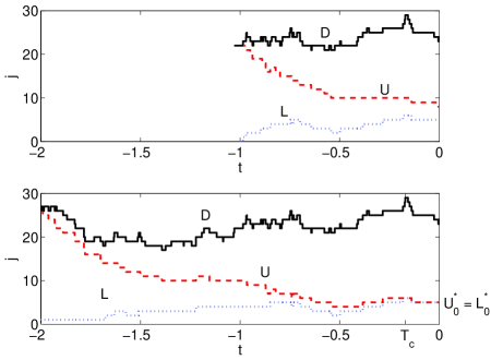
Figure 1: An illustrative run of the DCFTP-SSA for the Hill equation. The top panel shows the algorithm started from $t=-1$. Both the upper ($U$) and lower ($L$) are coupled to the dominating path ($D$) and here they fail to coalesce before $t=0$. The coupling implies that $U$ and $L$ can only change states if $D$ does so. In the lower panel, the algorithm is restarted from $t=-2$. Note that $D$ extends further into the past but the realization of $D$ in the interval $t\in[-1,0]$ is the same as above. In this case, coalescence occurs at $T_{c}=-0.17$ and the value $U^{*}_{0}=L^{*}_{0}$ is guaranteed to be a sample from the stationary solution of the Hill CME (Eq. 10).

Detailed application to the first order reaction

In order to illustrate the DCFTP-SSA, we study in detail the simple one-dimensional first order reaction, for which a full time-dependent analytical solution of the CME is available. This allows us to study the convergence of the algorithm, as compared to the standard SSA, and to explore the difference between two sources of error which often get entangled: finite sampling error and the mis-sampling error due to the fact that we may not have reached the true stationary distribution.

Consider the simple first order reaction, which has been used as a very simplified description of transcription and translation (18, 2):

$$\emptyset\ \xrightarrow{k}\ A\ \xrightarrow{1}\ \emptyset\quad\Longrightarrow\quad\dot{A}=k-A,$$ (3)

where species $A$ is created at a (normalized) constant rate $k$ from a source ($\emptyset$) and degraded to a sink ($\emptyset$). The corresponding CME is

$$\dot{P}_{j}=kP_{j-1}-kP_{j}+(j+1)P_{j+1}-jP_{j}\equiv(\mathbb{E}^{-1}-1)kP_{j}+(\mathbb{E}-1)jP_{j},$$ (4)

with $P_{j}$ denoting the probability of having $j$ molecules of $A$. $\mathbb{E}$ and $\mathbb{E}^{-1}$ are the step operators defined by van Kampen (13): $\mathbb{E}f(j)=f(j+1)$ and $\mathbb{E}^{-1}f(j)=f(j-1)$ for a function $f(j)$.

Equation 4 is one of a few CMEs for which the analytical expression of the stationary solution is known (42, 13): it is the Poisson distribution with parameter $\lambda=k$. More importantly for our purposes, one can obtain the full time-dependent solution of the CME (see Appendix A). For the usual initial condition with $0$ molecules, the time-dependent distribution $\mathbf{P}(t)$ is given by (see Fig. 2 inset):

$$P_{j}(t)\equiv P(j,t|0,0)=\frac{\exp\left(-k(1-e^{-t})\right)}{j!}\left[k(1-e^{-t})\right]^{j},$$ (5)

which converges to the correct stationary distribution as $t\to\infty$.

The mis-sampling error can be understood analytically in this simple example. If the standard SSA is used to estimate the stationary solution of the CME (Eq. 4), $N$ samples from independent SSA runs will be collected at a stopping time $t_{\rm SSA}$. This leads to the sampled distribution $\mathbf{P}_{\rm SSA}(N,t_{\rm SSA})$, which clearly converges to the stationary distribution $\mathbf{P}^{*}$ in the double limit $t_{\rm SSA},N\to\infty$. As $N$ is increased, with fixed $t_{\rm SSA}$, we sample with increasing Monte Carlo accuracy from $\mathbf{P}(t_{\rm SSA})$ given by Eq. 5 but not from the true stationary distribution $\mathbf{P}^{*}$. We therefore reach an error floor that cannot be broken. Using the analytical expression (Eq. 5), the asymptotic error floor $\epsilon_{E}^{*}(t_{\rm SSA})$ is shown to be

$$\epsilon_{E}^{*}(t_{\rm SSA})^{2} = \sum_{j=0}^{\infty}\left(P_{j}^{*}-P_{j}(t_{\rm SSA})\right)^{2}=\sum_{j=0}^{\infty}\left(\frac{e^{-k}k^{j}}{j!}-\frac{e^{-\alpha k}(\alpha k)^{j}}{j!}\right)^{2}$$ (6)

$$= I_{0}(2k)e^{-2k}-2I_{0}(2k\sqrt{\alpha})e^{-k-\alpha}+I_{0}(2k\alpha)e^{-2\alpha},$$

where $\alpha=1-e^{-t_{\rm SSA}}$ and $I_{0}(x)$ is the modified Bessel function of the first kind. Fig. 2 shows that the levelling-off of the Euclidean error for $\mathbf{P}_{\rm SSA}(N,t_{\rm SSA})$ is explained by the error floors calculated from Eq. 6.

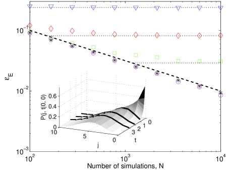
Figure 2: Comparison of the convergence of the DCFTP-SSA vs. the standard SSA for the first order reaction (Eq. 4) with $k=5$. We present the Euclidean error of the distribution as a function of the number of Monte Carlo runs $N$ for the DCFTP-SSA ($\ast$) and for the standard SSA with stopping times: $t_{\rm SSA}=1(\nabla),2(\Diamond),3(\Box),15(\bigcirc)$. Note that the error of the SSA runs converges to the asymptotic error floors for the different stopping times given by Eq. 6 (dotted lines). The dashed line corresponds to the $N^{-1/2}$ Monte Carlo scaling and shows the correct convergence of the DCFTP-SSA (and the SSA only when the stopping time is with very long). Each point is calculated from the mean of 100 different ensembles of $N$ samples, with numerical error bars smaller than the symbols. Inset: The full time-dependent solution of the first order reaction (Eq. 5) from a $\delta$-distribution initial condition. The distribution evolves towards a smoother Poisson distribution. The dark lines correspond to the distributions at $t=1,2,3$ used in the main panel.

This source of error is eliminated in a DCFTP-SSA formulation of this process. The key step is to find a reversible dominating process with known stationary distribution. In this example, it is clear that the best choice is to use the process (Eq. 4) itself, i.e., the $U$ and $D$ chains in Fig. 1 will be identical. Figure 2 shows the Euclidean error for the DCFTP-SSA sample distribution, which shows no flooring and the expected $N^{-1/2}$ scaling with the number of Monte Carlo runs (43). Equivalent results are obtained with other error measures for the sampled distribution, e.g., the Kullback-Leibler and Kolmogorov distances, and the $\chi^{2}$-goodness of fit.

The building blocks: networks and nonlinear elements

In order to extend our study to GRNs, we need to consider how to deal with two key ingredients: networks of reactions, and nonlinear elements of the Hill and Monod types.

Application to networks: Simple gene model of two coupled first order reactions

To showcase how to apply the DCFTP-SSA to networks of several species, we use a widely studied, simplified model of gene expression (15, 18, 17). In its simplest form, the model consists of two types of molecules: mRNA ($M$) and proteins ($R$), which are produced and depleted at constant rates. In addition, the mRNA catalyzes protein production through a linear enzymatic reaction:

The deterministic description is given by

$$\dot{M} = k_{M}-M$$

$$\dot{R} = k_{B}+k_{R}M-R,$$ (7)

and the corresponding CME is

$$\dot{P}_{M,R} = (\mathbb{E}^{-1}_{M}-1)k_{M}P_{M,R}+(\mathbb{E}_{M}-1)MP_{M,R}$$ (8)

$$+ (\mathbb{E}^{-1}_{R}-1)(k_{B}+k_{R}M)P_{M,R}+(\mathbb{E}_{R}-1)RP_{M,R}.$$

In fact, Eq. 8 has been solved: the stationary state of the CME of any general network of linear reactions is a multivariate Poisson distribution (17, 42). This means that, similarly to the one-dimensional first order reaction, the DCFTP-SSA is directly applicable to Eq. 8, since the reaction network is reversible and the multivariate Poisson stationary solution is itself a dominating process for the system. The existence of an analytical solution allows us to check how the accuracy of the DCFTP-SSA depends on the dimensionality of the system. Fig. 3 (inset) shows that the marginal distribution (for $M$) converges like the one dimensional reaction in Fig. 2, with similar error floors for the standard SSA. Note, however, that the joint distribution (Fig. 3) exhibits slower convergence of the standard SSA due to the higher dimensionality of the system, indicating the need for longer SSA runs to avoid mis-sampling from the true distribution. The DCFTP-SSA shows $N^{-1/2}$ Monte Carlo scaling with no error floors regardless of the dimensionality of the system.

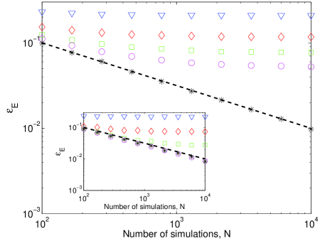
Figure 3: The effect of dimensionality on the convergence of the sampled distribution. The main panel shows the Euclidean error for the joint distribution of the linear gene model (Eq. 8) with $k_{M}=3$, $k_{R}=3$ and $k_{B}=1$. The open symbols correspond to the standard SSA with stopping times as in Fig. 2 while the DCFTP-SSA is marked by asterisks. The points are obtained by averaging over 100 ensembles of $N$ samples, with error bars contained within the symbols. The higher dimensionality and the topology of the network make the convergence of the standard SSA much slower for this case than for the one-dimensional first order reaction in Fig. 2. Note that the DCFTP-SSA is unaffected by error floors and shows $N^{-1/2}$ convergence, as given by the dashed line. Inset: Same as the main panel for the marginal distribution of the mRNA ($M$). In this case, the convergence is as for the one-dimensional linear reaction in Fig. 2. The difference between the convergence of the joint and marginal distributions is not surprising: the production of $R$ is downstream from $M$ and it is unlikely to reach the stationary level before $M$.

Non-linear elements: Hill and Monod reactions

The Hill reaction is widely used to model the sigmoidal (non-linear) characteristics of many biological processes and specifically those involved in genetic regulation (5, 4, 44). This model incorporates negative feedback, whereby the rate of creation of new molecules decreases as their concentration increases:

$$\emptyset\xrightarrow{f(A;\,k,\alpha)}A\xrightarrow{1}\emptyset\quad\Longrightarrow\quad\dot{A}=\frac{k}{\theta^{\alpha}+A^{\alpha}}-A,$$ (9)

where $f(A;k,\alpha)=k/(\theta^{\alpha}+A^{\alpha})$ is the state-dependent reaction rate, $k$ is the renormalized reaction constant and $\alpha$ is the cooperativity factor (45). Eq. 9 can be derived from elementary Law of Mass Action kinetics through elimination of variables (16). The corresponding CME is given by:

$$\dot{P}_{j}=(\mathbb{E}^{-1}-1)\frac{k}{\theta^{\alpha}+j^{\alpha}}P_{j}+(\mathbb{E}-1)jP_{j}.$$ (10)

It is usual to fix $\theta=1$ and we do so in the following. For the particular case $\alpha=1$, Eq. 9 reduces to the familiar Michaelis-Menten equation, for which we can obtain the following analytical expression for the stationary distribution (see Appendix B): $P^{*}_{j}=ck^{j}/(j!)^{2}$, where $c=1/I_{0}(2\sqrt{k})$ is a normalization constant.

The Monod reaction is used to model gene upregulation, as referred in particular to the auto-catalysis common in many eucaryotes (10, 44, 46). The reaction can be written as

$$\emptyset\xrightarrow{g(A;\,k,\alpha)}A\xrightarrow{1}\emptyset\quad\Longrightarrow\quad\dot{A}=\frac{kA^{\alpha}}{\theta^{\alpha}+A^{\alpha}}-A,$$ (11)

where $g(A;k,\alpha)=kA^{\alpha}/(\theta^{\alpha}+A^{\alpha})$ is the state-dependent reaction rate that encapsulates the positive feedback. The corresponding CME is given by

$$\dot{P}_{j}=(\mathbb{E}^{-1}-1)\frac{kj^{\alpha}}{\theta^{\alpha}+j^{\alpha}}P_{j}+(\mathbb{E}-1)jP_{j}.$$ (12)

Again, we fix $\theta=1$ in the following. The stationary distribution of the Monod CME (Eq. 12) with $\alpha=1$ can be obtained analytically (see Appendix B): $P^{*}_{j}=ck^{j}/j!$, with normalization constant $c=1/(e^{k}+k-1)$.

For general $\alpha$, no explicit solution for the stationary distribution of the CMEs Eq. 10 and Eq. 12 is known, and numerical methods are therefore necessary. Fortunately, the DCFTP-SSA is directly applicable to the reversible Hill and Monod CMEs: the first order reaction, studied in detail in the previous Section, can be used to produce a dominating process for both processes. To see this, note that Eq. 10 and Eq. 12 have birth rates that are bounded from above by $k$ at all times. It is thus straightforward to make sure that the upper and lower paths have rates that fulfill the requirements of the algorithm. As an illustration, Fig. 1 shows one DCFTP-SSA run for the Hill CME (Eq. 10), where $D$ corresponds to the dominating first order linear process (Eq. 4) and $U$ and $L$ are the coupled Hill processes (40, 39). Our detailed simulations of the Hill and Monod CMEs (data not shown) show $N^{-1/2}$ convergence of the DCFTP-SSA unaffected by the mis-sampling errors that can appear when using the standard SSA with short stopping times.

Application to nonlinear models of Gene Regulatory Networks

Our foregoing discussion clarifies why the DCFTP-SSA is applicable to reversible GRNs consisting of interconnected linear enzymatic, Hill and Monod birth reactions: it is possible to define a dominating process for these networks based on the associated linear network for which the stationary solution (a multivariate Poisson distribution) is known. We now apply our scheme to two recent, canonical examples of synthetic GRNs: a bistable genetic toggle switch (5), with a bimodal stationary distribution; and the repressilator (4), a simple synthetic oscillator.

Toggle switch: two coupled Hill equations

An important characteristic of biochemical networks is the possibility of multistability (5, 1, 14, 16, 18, 20, 47, 46), as exemplified by the toggle switch designed by Gardner et al by combining two mutually repressing genes (5, 16, 20, 11, 14). This leads to a bistable system with a sharp switching threshold:

A deterministic model can be derived using two coupled Hill-equations:

$$\dot{A} = \frac{k_{A}}{1+B^{\alpha}}-A$$

$$\dot{B} = \frac{k_{B}}{1+A^{\beta}}-B,$$ (13)

where $A$ and $B$ are the molecular numbers of the transcription factors. With appropriate cooperativity factors $\alpha,\beta>1$ and reaction constants $k_{A}$ and $k_{B}$, Eq. Toggle switch: two coupled Hill equations has two stable fixed points (5).

The corresponding CME is given by

$$\dot{P}_{A,B} = (\mathbb{E}^{-1}_{A}-1)\frac{k_{A}}{1+B^{\alpha}}P_{A,B}+(\mathbb{E}_{A}-1)AP_{A,B}$$ (14)

$$+ (\mathbb{E}^{-1}_{B}-1)\frac{k_{B}}{1+A^{\beta}}P_{A,B}+(\mathbb{E}_{B}-1)BP_{A,B}.$$

Based on our discussion above, it is easy to see that linear process with constant birth rates $k_{A}$ and $k_{B}$ will be a dominating process for Eq. 14. Since the Hill-function is anti-monotone, we must use a cross-over scheme for the updates to make sure that all initial conditions are sandwiched between the upper and lower paths, as described in Häggström and Nelander (41). We have applied the DCFTP-SSA to Eq. 14 to obtain the stationary distribution of the system, which is clearly bimodal (Fig. 4). Because there is no analytical solution in this case, we have checked the accuracy and convergence of the DCFTP-SSA against the approximate eigenvector method with excellent results (not shown).

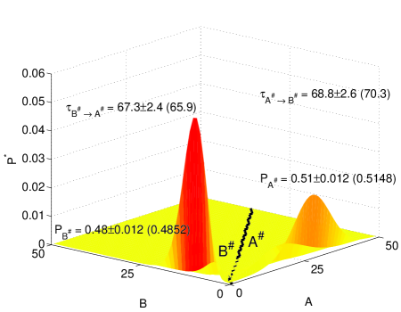
Figure 4: Stationary distribution for the toggle switch (Eq. 14) with parameters $k_{A}=30,k_{B}=10,\alpha=3,\beta=1$. The bimodality of the distribution leads to switching behavior. We have checked that the Euclidean error of the DCFTP-SSA sampled distribution decreases at the expected $N^{-1/2}$ rate (data not shown). The state space can be divided in two regions $A^{\#}$ and $B^{\#}$  corresponding to the two basins of attraction of the fixed points. The separatrix is found from the sign of the Fiedler eigenvector of the Laplacian (48) of the state space lattice. The probabilities $P_{A^{\#}}$ and $P_{B^{\#}}$ of finding the system in each basin computed with the DCFTP-SSA compare very well with those obtained with the approximate eigenvector method (in parenthesis). Similarly, the expected time to reach the separatrix averaged over all the states in each basin (37) calculated with the DCFTP-SSA (averaged over 25 ensembles, each consisting of 1000 samples) compare well with the approximate eigenvector method (in parenthesis).

Beyond certifying proper convergence, the DCFTP-SSA can be used to study properties of the network that need to be properly averaged over the stationary distribution. Consider the mean time for the system to switch from the basin of one fixed point $A^{\#}$ to the other $B^{\#}$, i.e., the escape time of the CME (Eq. 14). If the standard SSA were to be used, it would be unclear how to collect proper Monte Carlo statistics, since no certificate of stationarity exists. In contrast, we use a mixed scheme in which an initial DCFTP-SSA run is followed by a (faster) SSA run. The initial DCFTP-SSA run ensures that the initial condition for the SSA run is correctly sampled from the stationary distribution at $t=0$, in essence eliminating the ‘burn-in’ period. From that point onwards, a standard SSA run is performed to obtain statistics of the average time to cross the separatrix. The results are reported in Fig. 4.

In their experiments,  Gardner et al. (5) were able to induce faster $A^{\#}\to B^{\#}$ switching by reducing the downregulation capability of $A$ in the cellular environment. This can be mimicked by a modified CME in which the $A^{\beta}$-term in Eq. 14 is removed. If we run the SSA of this modified CME starting from the stationary distribution of the original system (Eq. 14), the escape time $\tau_{A^{\#}\to B^{\#}}$ becomes approximately two orders of magnitude smaller, in broad agreement with the experiment. In fact, it can be shown that the stationary distribution of the modified CME becomes unimodal, with no observable peak for species $A$.

Repressilator: six-dimensional system of linear enzymatic and Hill equations

The repressilator, a synthetic system of transcriptional regulators, is perhaps the simplest biochemical oscillator that has been implemented experimentally (4). It consists of three genes in a loop, in which the expression of one gene is inhibited by the product of another gene in succession (Fig. 5a):

$$\dot{M}_{i} = \frac{k_{M}}{1+R_{i+1}^{\alpha}}-d_{M}M_{i}$$

$$\dot{R}_{i} = k_{B}+k_{R}M_{i}-R_{i},\quad\quad i=0,1,2\;\;(\mathrm{mod}\,\,3).$$ (15)

Here $M_{i}$ are the mRNA levels (with production rate $k_{M}$ and degradation rate $d_{M}$) and $R_{i}$ are the corresponding proteins (with basal rate $k_{B}$ and linear production rate $k_{R}$). This model of the repressilator is therefore a network of linear enzymatic elements (Eq. 8) for the protein production terms and Hill reactions (Eq. 10) to modulate the production of mRNA. The deterministic system (Eq. Repressilator: six-dimensional system of linear enzymatic and Hill equations) has been shown to be oscillatory, with the concentrations of the three proteins peaking in succession (Fig. 5b, top panel).

The corresponding CME is given by

$$\dot{P}_{n} = \sum_{i=0}^{2}(\mathbb{E}^{-1}_{M_{i}}-1)\frac{k_{M}}{(1+R_{i+1}^{\alpha})}P_{n}+(\mathbb{E}_{M_{i}}-1)d_{M}M_{i}P_{n}$$ (16)

$$+ (\mathbb{E}^{-1}_{R_{i}}-1)(k_{B}+k_{R}M_{i})P_{n}+(\mathbb{E}_{R_{i}}-1)R_{i}P_{n},$$

where the shorthand $P_{n}$ denotes the state $P_{M_{0},M_{1},M_{2},R_{0},R_{1},R_{2}}$ and $i\,\,\mathrm{mod}\,\,3$. We have simulated this six dimensional system using the cross-over scheme described above: we use the DCFTP-SSA to discard the ‘burn-in period’, i.e., the time it takes for the Markov process to reach the stationary distribution, such that the initial conditions for the SSA runs are sampled from the stationary distribution. As a measure of the stationarity of our DCFTP-SSA initialized sampling, we have checked its ergodicity by establishing through an F-test that the average period and amplitude of several short simulations are statistically indistiguishible from those obtained from one long simulation.

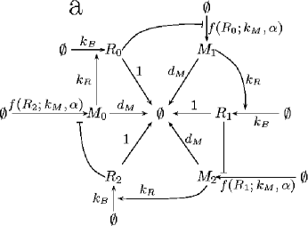
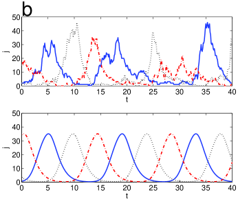
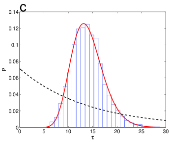
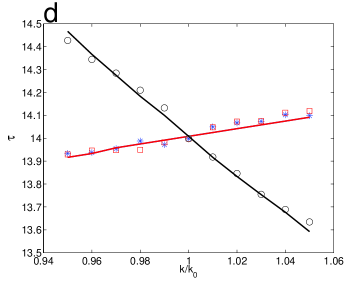
Figure 5: Analysis of the repressilator with $k_{M}=10$, $d_{M}=1$, $\alpha=2$, $k_{B}=1$, $k_{R}=3$. (a) Diagrammatic representation of the repressilator network showing the alternating positive and negative feedbacks. (b) Top: One SSA realization of the CME (Eq. 16) started from the stationary distribution showing the concentrations of the three proteins. The oscillations are very noisy and far from sinusoidal. The Fourier spectrum shows no distinguishable peaks (data not shown). Bottom: The corresponding deterministic solution (Eq. Repressilator: six-dimensional system of linear enzymatic and Hill equations) exhibits regular oscillations of the proteins in succession. (c) Distribution of the period $\tau$ at stationarity obtained from a long SSA run. The solid line corresponds to a best fit to a generalized Gamma distribution while the dotted line shows a Poisson distribution with the same mean. (d) Change of the period of the repressilator as a function of parameter variation. There is good agreement between the sensitivity of the stochastic system with respect to a $\pm 5\%$ change in $k_{M}$ ($\ast$), $k_{P}$ ($\Box$), and $d_{M}$ ($\bigcirc$), and the deterministic system (solid lines). The effect of $d_{M}$ on the duration of the period $\tau$ is greater and opposite to that of $k_{M}$ and $k_{P}$, which are similar.

As can be seen in the sample trajectory in Fig. 5b, the stochastic system is extremely noisy but it retains the overall oscillation of the genes in succession. The oscillations do not die out even for very long simulations and we have collected statistics of such long runs. Fig. 5c shows a robust feature of the oscillator: the distribution of the period is well fitted by a generalized Gamma distribution, which is characteristic of excitatory systems with a refractory period. The oscillatory behaviour is present for a wide range of the parameters $k_{M},k_{R},d_{M}$ (49), which could be modified experimentally. Fig. 5d summarizes our investigation of the robustness of the repressilator to parametric variation. Note the good agreement of the calculated mean period with the corresponding deterministic values. The simulations show that changes in parameters $k_{M}$ and $k_{R}$ produce a similar, small effect on the period. The system is, however, more sensitive to parametric changes in $d_{M}$. The evaluation of how these parametric variations could be used for the design of tunable and reliable oscillators will be the object of further study (50).

Discussion

In recent years, the importance of stochastic effects in gene regulation has been elegantly demonstrated through experiments. ¿From a theoretical perspective, such systems are usually analyzed numerically with the standard SSA. When studying stationary properties, this raises questions about the sampling of the stochastic process since the SSA does not provide explicit guarantees for convergence. One issue of interest for the use of the DCFTP-SSA is that the shape of the stationary distribution can be more important than the dimensionality of the system for the convergence of the stochastic simulations. For systems with smooth unimodal distributions, such as the repressilator, the SSA approaches the stationary distribution rapidly, regardless of the initial conditions. However, the ordinary SSA can be highly sensitive to initial conditions for systems with multimodal distributions, such as the toggle switch. In general, the SSA will converge rapidly to the nearest mode. If we are primarily interested in escape times, they can be estimated accurately by using the ordinary SSA started close to one of the modes. However, if the escape times from the modes are long and the ordinary SSA is used, we run the risk of mis-sampling the stationary distribution, specifically in important areas of low probability such as the separatrix. The DCFTP-SSA circumvents this problem but at the cost of longer coalescence times.

The guaranteed sampling provided by the DCFTP-SSA comes at an extra computational cost. In general, the coalescence time will depend on the topology of the network and the form of the reactions. However, the CPU overhead is in no way prohibitive and the DCFTP-SSA can be run on an ordinary desktop computer for the systems presented in this paper. An important theoretical feature of the DCFTP-SSA is the fact that its runtime is not bounded. As our simulations show, this feature does not seem to impose practical restrictions on the algorithm. If necessary, however, this issue can be resolved by using FMMR (51), another perfect sampling algorithm, which dispenses with variable stopping times by running the Markov chains for a fixed time and using rejection sampling to discard those simulations that have not reached the stationary distribution.

In its current form, the DCFTP-SSA can be applied to reversible systems of linear and nonlinear (anti-)monotonic unimolecular reactions for which there exists a dominating process with known stationary distribution. We note that the algorithm is applicable not only to networks of linear enzymatic, Hill and Monod birth reactions of standard form, but also to reactions whose rate equation is a rational function that can be dominated by a linear process. This condition is equivalent to requiring that the polynomial in the denominator of the propensity function have a higher degree than the polynomial in the numerator. These types of rational functions are frequently obtained as compound unimolecular rate laws to represent more complex enzymatic (44) or gene regulatory reactions (52). An example of such functions is the model for the $\lambda$-phage lysis-lysogeny switch (11, 14), which we have also simulated with the DCFTP-SSA (results not shown). Bimolecular and two-substrate enzymatic reactions are not included in this group and extending the DCFTP or CFTP to provide perfect sampling for the generic SSA of second order reactions will entail further research.

The DCFTP-SSA introduced here can be viewed as a reformulation and extension of the Gillespie algorithm that provides guaranteed sampling from stationarity for a generic class of systems relevant in GRNs, thereby removing a source of uncontrolled uncertainty from the simulations. By eliminating these extraneous sources of error, comparisons between the predictions of different stochastic models at stationarity can be performed more meaningfully. In the case of the repressilator, we provided an accurate numerical characterization of the stationary distribution for the period of this stochastic oscillator. Because stationarity is guaranteed, the characteristics of this distribution can be correlated with changes in the parameter values (as shown in Figure 5d) or compared with those of other genetic oscillators. This could be a useful tool for the analysis and design of synthetic transcriptional oscillators and will be the subject of future research.

Acknowledgments: We would like to thank Michael Elowitz for helpful comments about the repressilator, and Matthieu Bultelle, Matias Rantalainen, Vincent Rouilly and Sophia Yaliraki for valuable discussions and feedback. We are also grateful for the constructive comments made by one of the anonymous referees. Research funded by the EPSRC.

Appendix A Time-dependent solution of the Master Equation for the one-dimensional first-order reaction

The CME for the one-dimensional first order reaction (Eq. 4) has the same form as a homogenous birth-death process on the non-negative integers. It is also identical to the equation one obtains when studying the length of a $M/M/\infty$-queue with Poisson arrival and exponential service time (37). Associated with Eq. 4, there exists a family of orthogonal polynomials $\{\varphi_{j}(x)\}_{j=0}^{\infty}$ with the three term recurrence relation (53):

$$-x\varphi_{j}(x)=j\varphi_{j-1}(x)-(k+j)\varphi_{j}(x)+k\varphi_{j+1}(x),$$ (17)

where $\varphi_{0}(x)=1$ and $\varphi_{j}(x)=0$ for $j<0$. Karlin and McGregor showed that the recurrence relation (Eq. 17) leads to a spectral representation for $P_{ji}(t)$, the transition probability of going from state $i$ to state $j$ in time $t$:

$$P_{ji}(t)=P_{j}^{*}\int_{0}^{\infty}e^{-xt}\varphi_{i}(x)\varphi_{j}(x)\,d\phi(x),$$ (18)

where $\phi(x)$ is a positive measure on $x$ and $P_{j}^{*}$ is the stationary distribution.

The recurrence relation (Eq. 17) is satisfied by the Charlier polynomials with $\phi(x)$ equal to the Poisson distribution (53), i.e., the Charlier polynomials are a family of polynomials which are orthogonal with respect to the Poisson measure on a discrete lattice on the non-negative integers (54). The Charlier polynomial of order $i$, parameter $a$ and argument $x$ is denoted $C_{i}\big{(}x;a\big{)}$.

Using the following bilinear generating form of the Charlier polynomials (55)

$$\sum_{i=0}^{\infty}\frac{z^{k}}{k!}C_{i}\big{(}m;x\big{)}C_{i}\big{(}n;y\big{)}=e^{z}\left(1-\frac{z}{x}\right)^{m}\left(1-\frac{z}{y}\right)^{n}C_{m}\bigg{(}n;-\frac{(x-z)(y-z)}{z}\bigg{)},$$ (19)

Lee (56) showed that Eq. 18 can be simplified to give:

$$P_{ji}(t)=\frac{\exp\left(-k(1-e^{-t})\right)}{j!}\left[k(1-e^{-t})\right]^{j}\left(1-e^{-t}\right)^{i}C_{i}\bigg{(}j;-\frac{k(1-e^{-t})^{2}}{e^{-t}}\bigg{)}.$$ (20)

The important special case with initial condition given by a $\delta$-distribution at the origin can be simplified even further. If $P_{j}(0)=\delta(0)$, then $C_{0}(j;a)=1$ and Eq. 20 becomes

$$P(j,t|0,0)=\frac{\exp\left(-k(1-e^{-t})\right)}{j!}\left[k(1-e^{-t})\right]^{j}\equiv P_{j}(t),$$ (21)

which is a Poisson distribution with time-varying parameter $k(t)=k(1-e^{-t})$. Therefore, the stationary Poisson distribution $P^{*}_{j}=k^{j}e^{-k}/j!$ is approached exponentially fast.

Note that

$$\lim_{t\rightarrow\infty}P_{ji}(t)=\frac{e^{-k}k^{j}}{j!},$$ (22)

which is another way of showing that the stationary distribution the process is Poisson no matter what the initial condition is.

Appendix B Stationary solution of the Hill and Monod CMEs with $\alpha=1$

The stationary solution for the Hill CME (Eq. 10) with cooperativity factor $\alpha=1$, which is equivalent to the Michaelis-Menten reaction, can be obtained analytically. This reaction can be viewed as a non-linear birth-death process, which allows us to write the stationary distribution $P_{j}^{*}$ as (37)

$$P_{j}^{*}=c\frac{\lambda_{0}\lambda_{1}\cdots\lambda_{j-1}}{\mu_{1}\mu_{2}\cdots\mu_{j}},$$ (23)

where $\lambda_{i}$ and $\mu_{i}$ are the birth and death rates of state $i$ and $c$ is a normalization constant. Inserting the values from the CME (Eq. 10) we obtain

$$P_{j}^{*}=c^{-1}\frac{\frac{k}{\theta}\frac{k}{\theta+1}\cdots\frac{k}{\theta+j-1}}{j!}=c^{-1}\frac{k^{j}\Gamma(\theta+1)}{j!\Gamma(j+\theta)},$$ (24)

with normalization constant

$$c=\frac{\theta I_{\theta}(2\sqrt{k})+\sqrt{k}I_{1+\theta}(2\sqrt{k})}{k^{\theta/2}},$$

where $I_{\theta}(x)$ are Bessel functions. For the special case of $\theta=1$, we use a recurrence relation for Bessel functions to simplify the above result to $c_{0}^{-1}=I_{0}(\sqrt{2}k)$.

Consider now the Monod CME (12) with $\alpha=1$:

$$\dot{P}_{j}=\left\{\begin{array}[]{ll}(\mathbb{E}^{-1}-1)\frac{kj}{\theta+j}P_{j}+(\mathbb{E}-1)jP_{j}&\textrm{if $j>1$}\\ k&\textrm{if $j=0$}.\end{array}\right.$$

Note that the birth rate of the state $j=0$ is modified to avoid it becoming absorbing. Using the same strategy as for the Michaelis-Menten CME above, one can find the stationary distribution

$$P_{j}^{*}=c\frac{k\frac{k}{\theta+1}\cdots\frac{k(j-1)}{\theta+j-1}}{j!}=c\frac{k^{j}\Gamma(\theta+1)}{j\Gamma(j+\theta)},$$ (25)

with normalization constant $c=k\left(1+{}_{1}F_{1}(2,1+\theta,k)\right)$, where ${}_{1}F_{1}$ is Gauss’ hypergeometric function.

References

- Acar et al. (2005) Acar, M., A. Becskei, and A. van Oudenaarden. 2005. Enhancement of cellular memory by reducing stochastic transitions. Nature 435:228–232.
- Austin et al. (2006) Austin, D., M. Allen, J. McCollum, R. Dar, J. Wilgus, G. Sayler, N. Samatova, C. Cox, and M. Simpson. 2006. Gene network shaping of inherent noise spectra. Nature 439:608–611.
- Blake et al. (2003) Blake, W. J., M. Kaern, C. R. Cantor, and J. Collins. 2003. Noise in eukaryotic gene expression. Nature 422:633–637.
- Elowitz and Leibler (2000) Elowitz, M. B., and S. Leibler. 2000. A synthetic oscillatory network of transcriptional regulators. Nature 403:335–339.
- Gardner et al. (2000) Gardner, T. S., C. R. Cantor, and J. J. Collins. 2000. Construction of a genetic toggle switch in escherichia coli. Nature 403:339–343.
- Pedraza and van Oudenaarden (2005) Pedraza, J. M., and A. van Oudenaarden. 2005. Noise propagation in gene networks. Science 307:1965–1969.
- Volfson et al. (2006) Volfson, D., J. Marciniak, W. J. Blake, N. Ostroff, L. S. Tsimring, and J. Hasty. 2006. Origins of extrinsic variability in eukaryotic gene expression. Nature 439:861–864.
- Cai et al. (2006) Cai, L., N. Friedman, and X. S. Xie. 2006. Stochastic protein expression in individual cells at the single molecule level. Nature 440:358–362.
- Fung et al. (2005) Fung, E., W. W. Wong, J. K. Suen, T. Butler, S. gu Lee, and J. C. Liao. 2005. A synthetic gene-metabolic oscillator. Nature 435:118–122.
- Beckskei et al. (2001) Beckskei, A., B. Séraphin, and L. Serrano. 2001. Positive feedback in eukaryotic gene networks: cell differentiation by graded to binary response conversion. The EMBO Journal 20:2528–2535.
- McAdams and Arkin (1997) McAdams, H. H., and A. Arkin. 1997. Stochastic mechanisms in gene expression. Proceedings of the National Academy of Sciences 94:814–819.
- Elf et al. (2003) Elf, J., J. Paulsson, O. G. Berg, and M. ns Ehrenberg. 2003. Near-critical phenomena in intracellular metabolite pools. Biophysical Journal 84:154–170.
- van Kampen (1992) van Kampen, N. G. 1992. Stochastic processes in physics and chemistry. 2nd edition. Elsevier.
- Hasty et al. (2000) Hasty, J., J. Pradines, M. Dolnik, and J. J. Collins. 2000. Noise based switches and amplifiers for gene expression. Proceedings of the National Academy of Sciences 97:2075– 2080.
- Kaern et al. (2005) Kaern, M., T. C. Elston, W. J. Blake, and J. J. Collins. 2005. Stochasticity in gene expression: from theories to phenotypes. Nature reviews 6:451–464.
- Kepler and Elston (2001) Kepler, T. B., and T. C. Elston. 2001. Stochasticity in transcriptional regulation: Origins, consequences and mathematical representations. Biophysical Journal 81:3116–3136.
- Paulsson (2004) Paulsson, J. 2004. Summing up the noise in gene networks. Nature 427:415–419.
- Thattai and van Oudenaarden (2001) Thattai, M., and A. van Oudenaarden. 2001. Intrinsic noise in gene regulatory networks. Proceedings of the National Academy of Sciences 98:8614–8619.
- Bratsun et al. (2005) Bratsun, D., D. Volfson, L. S. Tsimring, and J. Hasty. 2005. Delay-induced stochastic oscillations in gene regulation. Proceedings of the National Academy of Sciences 102:14593–14598.
- Erban et al. (2006) Erban, R., I. G. Kevrekidis, D. Adalsteinsson, and T. C. Elston. 2006. Gene regulatory networks: A coarse-grained, equation-free approach to multiscale computation. Journal of Chemical Physics 124. 084106.
- Swain and Elowitz (2002) Swain, P. S., and M. B. Elowitz. 2002. Intrinsic and extrinsic contributions to stochasitcity in gene expression. Proceedings of the National Academy of Sciences 99:12795–12800.
- Lai et al. (2004) Lai, K., M. J. Robertson, and D. Schaffer. 2004. The sonic hedgehog signalling system as a bistable genetic switch. Biophysical Journal 86:2748–2757.
- Samoilov et al. (2005) Samoilov, M., S. Plyasunov, and A. P. Arkin. 2005. Stochastic amplification and signaling in enzymatic futile cycles through noise-induced bistability with oscillations. Proceedings of the National Academy of Sciences 102:2310–2315.
- Elf and ns Ehrenberg (2003) Elf, J., and M. ns Ehrenberg. 2003. Fast evaluation of fluctuations in biochemical networks with the linear noise approximation. Genome Research 13:2475–2484.
- Delbrück (1940) Delbrück, M. 1940. Statistical fluctuations in autocatalytic reactions. Journal of Chemical Physics 8:120–124.
- McQuarrie (1967) McQuarrie, D. 1967. Stochastic approach to chemical kinetics. Journal of Applied Probability 4:413–478.
- Paulsson (2005) Paulsson, J. 2005. Models of stochastic gene expression. Physics of life reviews 2:157–175.
- Gillespie (1976) Gillespie, D. T. 1976. A general method for numerically simulating the stochastic time evolution of coupled chemical reactions. Journal of Computational Physics 22:403–434.
- Doob (1945) Doob, J. L. 1945. Markoff chains - denumerable case. Transactions of the American Mathematical Society 58:455–473.
- Gillespie (1992) Gillespie, D. T. 1992. A rigorous derivation of the chemical master equation. Physica A 188:404–425.
- Stundzia and Lumsden (1996) Stundzia, A. B., and C. J. Lumsden. 1996. Stochastic simulation of coupled reaction-diffusion processes. Journal of Computational Physics 127:196–207.
- Elf and Ehrenberg (2004) Elf, J., and M. Ehrenberg. 2004. Spontaneous separation of bi-stable biochemical systems into spatial domains of opposite phases. IEE Systems Biology 1:230–236.
- Gibson and Bruck (2000) Gibson, M. A., and J. Bruck. 2000. Efficient exact stochastic simulation of chemical systems with many species and many channels. Journal of Physical Chemistry A 104:1876–1899.
- Cao et al. (2006) Cao, Y., D. T. Gillespie, and L. R. Petzold. 2006. Efficient step size selection for the tau-leaping simulation method. Journal of Chemical Physics 124. 044109.
- Tomioka et al. (2004) Tomioka, R., H. Kimura, T. J. Kobayashi, and K. Aihara. 2004. Multivariate analysis of noise in genetic regulatory networks. Journal of Theoretical Biology 229:501–521.
- Kummer et al. (2005) Kummer, U., B. Krajnc, J. Pahle, A. K. Green, C. J. Dixon, and M. Marhl. 2005. Transition from stochastic to deterministic behavior in calcium oscillations. Biophysical Journal 89:1603–1611.
- Norris (1999) Norris, J. R. 1999. Markov chains. Cambridge University Press.
- Propp and Wilson (1996) Propp, J. G., and D. B. Wilson. 1996. Exact sampling with coupled Markov chains and applications to statistical mechanics. Random structures and algorithms 9:223–252.
- Kendall (1997) Kendall, W. S. 1997. Perfect simulation for spatial point processes. In Bulletin ISI, 51st session proceedings, volume 3. 163–166.
- Thönnes (2000) Thönnes, E. 2000. A primer on perfect simulation. In Springer Lecture Notes in Physics, K. R. Mecke, and D. Stoyan, editors, volume 554. Springer, 349–378.
- Häggström and Nelander (1998) Häggström, O., and K. Nelander. 1998. Exact sampling from anti-monotone systems. Statistica Neerlandica 52:360–380.
- Gadgil et al. (2005) Gadgil, C., C.-H. Lee, and H. G. Othmer. 2005. A stochastic analysis of first-order reaction networks. Bulletin of Mathematical Biology 67:901–946.
- Shreider (1966) Shreider, Y. A. 1966. The Monte Carlo Method. Pergamon Press.
- Cornish-Bowden (2004) Cornish-Bowden, A. 2004. Fundamentals of Enzyme Kinetics. 3rd edition. Portland Press.
- Rosenfeld et al. (2002) Rosenfeld, N., M. B. Elowitz, and U. Alon. 2002. Negative autoregulation speeds up the response times of transcription networks. Journal Of Molecular Biology 323:785–793.
- Xiong and Jr (2003) Xiong, W., and J. E. F. Jr. 2003. A positive-feedback-based bistable ’memory module’ that governs a cell fate decision. Nature 426:460–465.
- Craciun et al. (2006) Craciun, G., Y. Tang, and M. Feinberg. 2006. Understanding bistability in complex enzyme-driven reaction networks. Proceedings of the National Academy of Sciences 103:8697–8702.
- Chung (1997) Chung, F. R. K. 1997. Spectral graph theory. American Mathematical Society.
- Scott et al. (2006) Scott, M., B. Ingalls, and M. Kaern. 2006. Estimation of intrinsic and extrinsic noise in models of nonlinear genetic networks. Chaos :026107.
- Tomshine and Kaznessis (2006) Tomshine, J., and Y. N. Kaznessis. 2006. Optimization of a stochastically simulated gene network model via simulated annealing. Biophysical Journal 91:3196–3205.
- Fill et al. (2000) Fill, J. A., M. Machida, D. J. Murdoch, and J. S. Rosenthal. 2000. Extension of Fill’s perfect rejection sampling algorithm to general chains. Random Structures and Algorithms 9:223–252.
- Widder et al. (2005) Widder, S., J. Schicho, and P. Schuster. 2005. Dynamic patterns of gene regulation I: simple two gene systems. Http://www.santafe.edu/research/publications/wpabstract/200603007.
- Karlin and McGregor (1955) Karlin, S., and J. McGregor. 1955. Representation of a class of stochastic processes. Proceedings of the National Academy of Sciences 41:387–391.
- Nikiforov et al. (1991) Nikiforov, A. F., S. K. Suslov, and V. B. Uvarov. 1991. Classical orthogonal polynomials of a discrete variable. Springer-Verlag.
- Meixner (1939) Meixner, J. 1939. Erzeugende funktionen der Charlierschen polynome. Mathematische Zeitschrift 44:531–535.
- Lee (1997) Lee, P.-A. 1997. Markov processes and a multiple generating function of product of generalized Laguerre polynomials. Journal of Physics A 30:373–377.