Cucker-Smale Flocking under Hierarchical Leadership

Abstract

A mathematical theory on flocking serves the foundation for several ubiquitous multi-agent phenomena in biology, ecology, sensor networks, economy, as well as social behavior like language emergence and evolution. Directly inspired by the recent fundamental works of Cucker and Smale on the construction and analysis of a generic flocking model, we study the emergent behavior of Cucker-Smale flocking under hierarchical leadership. The rates of convergence towards asymptotically coherent group patterns in different scenarios are established.

The consistent convergence towards coherent patterns may well reveal the advantages and necessities of having leaders and leadership in a complex (biological, technological, economic, or social) system with sufficient intelligence.

Key words. Bio-flocking, leaders, leadership, Cucker-Smale model, dynamic graphs, graph Laplacian, Fiedler number, convergence, perturbation, free will.

AMS subject classification. 92D50, 92D40, 91D30, 91C20.

1 Introduction and Motivations

1.1 General Background on Flocking

Flocking, a universal phenomenon of multi-agent interactions, has gained increasing interest from various research communities in biology, ecology, robotics and control theory, sensor networks, as well as sociology and economics.

1. (Biology and Ecology) The emergent behavior of bird flocks, fish schools, wolf packs, elephant herds, or bacteria aggregations, for example, has long been a major research topic in population and behavioral biology and ecology [8, 3, 4, 5, 9, 14, 20, 21].

2. (Robotics and Control) The coordination and cooperation among multiple mobile agents (robots or sensors) have been playing central roles in sensor networking, with broad applications in military, environmental control, or various field tasks [11, 22].

3. (Economy and Languages) Emergent economic behavior, such as a common belief in a price system in a complex market environment, is also intrinsically connected to flocking. The emergence of a common language in primitive societies is yet another example of a coherent collective behavior emerging within a complex system [5, 6].

The present work can largely be categorized into the biology realm, and has been directly inspired by the recent mathematical works of Cucker and Smale [4, 5], as the title suggests. Mathematical abstraction and rigorous analysis are more focused herein than actual biological or physical realizability or feasibility. As in physics, the study of idealized models can often shed light on various observed patterns in the real world, if  such models can indeed catch the very essence.

In biology and physics, the main goal of flocking study is to be able to interpret, model, analyze, predict and simulate various flocking or multi-agent aggregating behavior. Most existing works have been focusing on modeling and simulation [12, 23]. See, for example, the several important models investigated by Flierl et al. [9] (and their stochastic formulation). The more recent paper of Parrish et al. [15] also provides a comprehensive comparison among some major existing models and their governing variables (in the context of fish schooling). Quantitative analysis (as in [4, 5, 11]) on the asymptotic rates of emergence and convergence, on the other hand, has been relatively rare.

Mathematical efforts are gradually gaining strength in this multidisciplinary area. In the continuum limit, for example, there have been several recent efforts made by Bertozzi’s group [20, 21], in which global swarming (i.e., with densely populated agents) patterns are modeled and analyzed via suitable spatiotemporal differential equations. Discrete-to-continuum limits of interacting particle systems have also been investigated by the same group [1, 8] recently. Consistent and generic mathematical analysis has been very much in an early stage for many biological aggregation phenomena. In the current paper, following the recent remarkable works of Cucker and Smale [4, 5] on flocking analysis, we attempt to make further extension along the same line.

1.2 Cucker-Smale Flocking Model

Given a flock of $k$ agents (birds, fish, wolves, etc) labeled by $i=1,2,\dots,k$, the Cucker-Smale flocking model is specified by the nonlinear autonomous dynamic system:

$$\begin{cases}\dot{x}_{i}(t)=v_{i},\\ \dot{v}_{i}(t)=\sum_{j\in{\mathcal{L}}(i)}a_{ij}(x)(v_{j}-v_{i}),\qquad i=1:k,t>0,\end{cases}$$ (1)

where $x_{i}(t)$ and $v_{i}(t)$ are 3D (3 dimensional, which is non-essential) position and velocity vectors at time $t$, $x=(x_{1},\dots,x_{k})\in({\mathbb{R}}^{3})^{k}$, and ${\mathcal{L}}(i)\subseteq\{1,\cdots k\}$ denotes the subgroup of agents that directly influence agent $i$. Furthermore, the connectivity coefficients $a_{ij}(x)$ are in the form of

$$a_{ij}(x)=w(|x_{i}-x_{j}|^{2}),\qquad\mbox{for some nonnegative weight profile $w(y)$.}$$

In the current paper, by Cucker-Smale flocking model, we require as in [4, 5] that the interaction weight function $w(y)$ takes the form of:

$$w(y)=\frac{H}{(1+y)^{\beta}},\qquad\mbox{or}\qquad w(y)\geq\frac{H}{(1+y)^{\beta}},$$ (2)

where $H$ and $\beta$ are two positive system parameters. One shall see that the two ($=$ vs. $\geq$) make no difference for the analysis hereafter as long as $w(y)$ is bounded and sufficiently smooth (also see [4]). We also must point out that this model has been put in a more general and abstract setting in the subsequent work of Cucker and Smale [5].

The look of the system (1) is not entirely new. For example, the 2D model studied by Vicsek et al. [23] is very similar in which $v_{i}$’s share the same magnitude (or speed) while their heading directions $\theta_{i}$’s satisfy a similar set of equations.

It is the particular choice of the connectivity coefficients in (2) that has made the Cucker-Smale model mathematically more attractive. Vicsek et al.’s model (in discrete time) [23] can be considered as taking the following cut-off weight function:

$$w(y)=w_{r}(y)=1_{y\leq r^{2}}(y),\qquad{\mathcal{L}}(i)\equiv\{1,\dots,k\},\quad\forall i.$$

That is, two distinct agents $x_{i}$ and $x_{j}$ interact if and only if they are within a distance of $r>0$, which is assigned a priori and fixed throughout. The lack of long-range interactions has made the model very difficult to analyze. For example, the remarkable efforts of Jadbabaie et al. [11] on emergence analysis avoided the actual dynamic dependence of $a_{ij}$ on the configuration $x$, but instead, they focused on an altered setting that involves switching controls.

The main results of Cucker and Smale [4] can be summarized as follows: when $\beta<1/2$, the flock converge to some translating rigid structure (moving at a constant velocity) unconditionally, i.e., regardless the initial configuration; and when $\beta\geq 1/2$, the initial velocities and positions have to satisfy certain compatible conditions so that the entire flock can converge asymptotically.

In summary, in the modeling and analysis of Cucker and Smale [4, 5], not only are the conditions for pattern emergence easily verifiable (i.e., by checking the initial conditions), but the role of long-range interaction is also clearly quantified. A smaller $\beta$ signifies more intense long-range interactions among agents while a bigger $\beta$ leads to much weaker ones. It has been shown that the critical exponent $\beta_{c}=1/2$ is sharp and necessary. Previously, the connection between global pattern emergence and individual action rules has often only been observed experimentally or addressed empirically (Vicsek et al. [23], for example, experimentally observed phase transition induced by population density $\rho$ and random fluctuation $\eta$. A higher density corresponds to more interaction among agents, or loosely, smaller $\beta$ in the Cucker-Smale model.)

1.3 Motivations and Main Results of Current Work

In the current work, we investigate the emergent behavior of Cucker-Smale flocking under hierarchical leadership (HL), which will be defined in detail in the next section.

Roughly, an HL flock is one whose members can be ordered in such a way that lower-rank agents are led and only led by some agents of higher ranks. As explained in more details in Section 2, for HL flocks, it is often either nontrivial or impossible to define a “fixed” inner product so that the Fiedler number of the associated (graph) Laplacian can be exploited, which is the key to the original work of Cucker and Smale [4] and its subsequent generalization [5]. The current work thus takes a somewhat different approach in order to fully benefit from the characteristic structures of HL.

As far as applications are concerned, there are two types of HL: passive and active ones.

1. (Passive/Transient Leadership)

   1. (Disturbed Bird Flocks) In nature, certain types of leadership emerge in a transient and dynamic fashion and is often prompted by a specific environment. For a disturbed bird flock at rest, for example, the bird that first senses the approach of an unexpected pedestrian or predator often takes flight first, warns others, and first gains full speed, and consequently flies ahead of the entire flock and serves as a virtual leader.

   2. (Driving in a Traffic) During rush hours, each individual driver mainly manoeuvres according to the moving patterns of several cars right ahead in the visual field. Thus a chain of leadership naturally arises and extends linearly along the traffic. The leadership here is also prompted by the environment rather than being intrinsic among the stranger drivers.

2. (Active/Intrinsic Leadership)

   1. (Governmental/Miltiary Hierarchies) Such hierarchical leadership is inherent in various social groups or structures, and often leads to more efficient management. Examples include, the chain of President-Governor-Mayor in the governmental system, and the chain of command from the Commander in Chief all the way down to a soldier.

   2. (Social Animals) For some social animals such as monkeys, wolves, or elephants [3], the group or social status of each member is clearly recognized by others and stably maintained, and guides the action of each individual in the hierarchies. (See also the recent work of Couzin et al. [3] for non-hierarchical but “effective” leadership.)

Our main results are the three theorems summarized below. All HL flocks are assumed to have Cucker-Smale connectivity introduced in the preceding subsection.

1. (Section 3) For an HL $(k+1)$-flock marching at a sufficiently small discrete time step $h$, under the similar classification scheme according to $\beta<\beta_{c}$, $=\beta_{c}$, or $>\beta_{c}$, as in Cucker and Smale [4, 5], the velocities of the flock converge at a rate of $O(\rho_{h}^{n}n^{k-1})$, where the factor $\rho_{h}\in(0,1)$ only depends on $h$, system parameters, and the initial configuration of the flock. The critical exponent is given by $\beta_{c}=1/(2k)$, instead of $\beta_{c}=1/2$ in the original work of Cucker and Smale [4]. (For a $2$-flock (with $k=1$) they are the same. For $k>1$, the $\beta_{c}$ herein could be over restrictive and due to the deficiency of the particular methodology adopted.)

2. (Section 4) For an HL flock under continuous-time dynamics, when $\beta<1/2$, there exists some $B>0$, such that the velocities of the flock converge at an exponential rate of $O(e^{-Bt})$. The constant $B$ only depends on the system parameters and the initial configuration of the flock. (From the simple calculation on an HL 2-flock, $\beta_{c}=1/2$ is sharp in order to achieve unconditional convergence.)

3. (Section 5) For an HL $(k+1)$-flock $[0,1,\dots,k]$ of which the overall leader agent 0 takes a free-will acceleration $\dot{v}_{0}=f(t)$ (thus the system is no longer autonomous), as long as the overall leader behaves moderately so that $f(t)=O((1+t)^{-\mu})$ for some $\mu>k$, the velocities of the flock will still converge at a rate of $O((1+t)^{-(\mu-k)})$ when $\beta<1/2$. (By (ii) where $f\equiv 0$, $\beta_{c}=1/2$ is again sharp for unconditional convergence.)

We also mention that Jadbabaie et al. [11] also studied (under discrete time and working with Vicsek et al.’s orientation model [23]) the effect of a single leader moving at a fixed constant velocity. As mentioned above, due to the difficulty in dealing with configuration-dependent dynamics, the authors switched to the study of an altered control problem (under the assumption of intermittent joint connectivity).

In addition to the three main sections mentioned above, definitions and further detailed background will be introduced in Section 2. The conclusion is drawn in Section 6.

2 HL Flocks, and Definability of Compatible Inner Products

2.1 Flocks under Hierarchical Leadership (HL Flocks)

Definition 1 (An HL Flock)

A $(k+1)$-flock is said to be under hierarchical leadership, if the agents (birds, fish, wolves, etc.) can be labeled as $[0,1,\dots,k]$, such that

1. $a_{ij}=a_{\mbox{agent $i$ led by $j$}}\;\neq 0$ implies that $j<i$; and

2. if we define the leader set of each agent $i$ by

   $${\mathcal{L}}(i)=\{j\mid a_{ij}>0\},$$

   then for any $i>0$, ${\mathcal{L}}(i)\neq\varnothing$ (non-empty).

If so, the flock is called an HL flock.

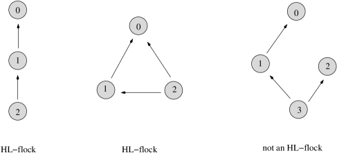
Figure 1: Two examples of HL flocks and one example of a non-HL flock. The arrow $i\to j$ means that agent $i$ is led by agent $j$, or equivalently, $a_{ij}>0$. Visually, it means that $i$ looks up to $j$.

Notice that the second condition requires that, except for agent 0, all the others must be subject to some leadership. On the other hand, the first condition implies that ${\mathcal{L}}(0)=\varnothing$. Thus agent 0 is the overall leader (direct or indirect) for the entire flock. Figure 1 depicts the connectivity structure of two HL flocks and one non-HL flock.

Proposition 1 (Connectivity Matrix of an HL Flock)

A $(k+1)$-flock is an HL flock if and only if after some ordered labeling $[0,1,\dots,k]$, the connectivity matrix $K=(a_{ij})_{0\leq i,j\leq k}$ is lower triangular, and for any row $i>0$, there exists at least one positive off-diagonal element $a_{ij}$.

Subject to convenience, in what follows a generic HL flock shall be denoted by either $[0,1,\cdots,k]$ or $[1,\cdots,k]$. As in Cucker-Smale [4] or Chung [2], define the graph Laplacian matrix by

$$L=D-K,\qquad D=\mbox{diag}(d_{0},\dots,d_{k}),\qquad d_{i}=\sum_{j}a_{ij}.$$ (3)

Similarly, define the two (non-orthogonally) complementing subspaces of ${\mathbb{R}}^{k+1}$:

$$\Delta=\mbox{span}\left\{\begin{pmatrix}1\\ \vdots\\ 1\end{pmatrix}_{k+1}\right\},\quad\mbox{and}\quad{\mathbb{R}}^{k}=\left\{\begin{pmatrix}0\\ x_{1}\\ \vdots\\ x_{k}\end{pmatrix}\mid x_{i}^{\prime}s\in{\mathbb{R}}\right\}.$$

Then it is easy to see that

$$\Delta=\mbox{Ker}(L),\qquad\mbox{and ${\mathbb{R}}^{k}=\mbox{Range}(L)$ is $L$-invariant.}$$

Notice that the kernel assertion is directly guaranteed by the second condition of an HL flock, without which the kernel could be larger.

From now one, as in Cucker and Smale [4, 5], we shall only consider the restriction of the Laplacian on the reduced space ${\mathbb{R}}^{k}$. Then it becomes nonsingular, and shall still be denoted by $L$ for convenience. We also must point out that when applied to actual flocking, the reduced Laplacian $L$ is applied to ${\mathbb{R}}^{3k}$ (instead of ${\mathbb{R}}^{k}$) via the three spatial dimensions individually.

2.2 Definability of Compatible Inner Products

The general framework of Cucker and Smale [4] relies upon the Fiedler number of the Laplacian operator $L$, i.e., the smallest positive eigenvalue in the reduced space. In particular, it assumes the existence of a fixed inner product $\langle\cdot,\;\cdot\rangle$ such that

$$\langle Lv,\;v\rangle\geq\xi\langle v,\;v\rangle,\qquad\mbox{for any}\;v\in{\mathbb{R}}^{k}.$$ (4)

Then an a priori   lower bound on $\xi=\xi(x)$ constitutes the core to the convergence results established by Cucker and Smale [4, 5]. Below we show, however, that such inner products could fail to exist for non-symmetric systems like HL flocks.

Theorem 1

Consider the special HL $(k+1)$-flock $[0,1,\dots,k]$ such that ${\mathcal{L}}(i)=\{i-1\}$ for $i>0$, and an instant when $a_{i,i-1}\equiv a$ for some fixed $a>0$ and any $i>0$. Then the smallest eigenvalue is $\xi=a$, but there exists no inner product $\langle\cdot,\;\cdot\rangle$ in the reduced space ${\mathbb{R}}^{k}$ such that

$$\langle Lv,\;v\rangle\geq a\langle v,\;v\rangle,\qquad v\in{\mathbb{R}}^{k}.$$

Proof. It is easy to see that the (reduced) Laplacian $L$ is given by

$$L=L_{a}=\begin{bmatrix}a&0&\dots&0&0\\ -a&a&\dots&0&0\\ \vdots&\vdots&\ddots&\vdots&\vdots\\ 0&0&\dots&-a&a\end{bmatrix}_{k\times k}.$$

In particular, $L_{a}=aL_{1}$, and it suffices to prove the case when $a=1$. If such an inner did exist, one would have

$$\langle L_{1}v,\;v\rangle\geq\langle v,\;v\rangle,\qquad\mbox{or}\;\;\langle Jv,\;v\rangle\geq 0,$$

where $J=L_{1}-Id$. Notice that $Jv=(0,-z_{1},\dots,-z_{k-1})^{T}$ for $v=(z_{1},\dots,z_{k})^{T}$.

Let $e_{i}^{\prime}s$ denote the canonical basis of ${\mathbb{R}}^{k}$, and define

$$G=(g_{ij})=(\langle e_{i},\;e_{j}\rangle)_{k\times k}$$

to be the associated Grammian matrix of the inner product. Then $G$ must be positive definite. For any $v=(z_{1},\cdots,z_{k})^{T}$, one has

$$\langle v,\;Jv\rangle=v^{T}G\cdot Jv=(z_{1},\dots,z_{k})(g_{ij})(0,-z_{1},\dots,-z_{k-1})^{T}.$$

Consider a special vector in the form of $w=w_{t}=(0,\dots,0,1,t)^{T}\in{\mathbb{R}}^{k}$. Then

$$\langle w_{t},\;Jw_{t}\rangle=(0,\dots,0,1,t)(g_{ij})(0,\dots,0,1)^{T}=g_{k-1,k}+g_{k,k}t.$$

Notice that $g_{k,k}=\langle e_{k},\;e_{k}\rangle>0$. Then for any

$$t<-\frac{\left|g_{k-1,k}\right|}{g_{k,k}},$$

one must have $\langle w_{t},\;Jw_{t}\rangle<0$, which is contradictory. $\blacksquare$

Even when such compatible inner products do exist, for a general non-symmetric flock, they often depend on the configuration of the flock, and are thus time-dependent. This causes much inconvenience or a potential impasse for the Cucker-Smale approach in [4, 5]. The efforts in the current work follow a different approach by exploiting the specific structures of HL flocks.

3 Discrete-Time Emergence

Recall that in the continuous time, the Cucker-Smale flocking model is given by

$$\begin{cases}\dot{x}=v,\\ \dot{v}=-L_{x}v,\qquad t>0,\end{cases}$$ (5)

Where the reduced Laplacian $L=L_{x}$ is defined as in (3) and both $x$ and $v$ are considered in the reduced (quotient) space. For a $(k+1)$-flock, both of them belong to ${\mathbb{R}}^{3k}$.

Fixing a discrete time step $h>0$. Define

$$x[n]=x(nh),\qquad v[n]=v(nh),\quad\mbox{and}\quad L_{n}=L_{x[n]}.$$

(Note: the parenthesis-bracket correspondence follows the convention in digital signal processing [19].) Then the continuous-time system (5) is discretized to

$$\begin{cases}x[n+1]=x[n]+hv[n],\\ v[n+1]=S[n]v[n],\qquad n=0,1,\cdots\end{cases}$$ (6)

where $S[n]=S^{h}[n]=Id-hL_{n}$.

For an HL $(k+1)$-flock $[0,1,\dots,k]$ , recall that the reduced Laplacian is given by

$$L_{n}=\begin{bmatrix}d_{1}[n]&0&\dots&0&0\\ -a_{21}[n]&d_{2}[n]&\dots&0&0\\ \vdots&\vdots&\ddots&\vdots&\vdots\\ -a_{k1}[n]&-a_{k2}[n]&\dots&-a_{k,k-1}[n]&d_{k}[n]\end{bmatrix}_{k\times k}.$$ (7)

For $i>0$, since the leader set ${\mathcal{L}}(i)\neq\varnothing$, we have

$$d_{i}[n]=\sum_{j=1}^{k}a_{ij}[n]=\sum_{j\in{\mathcal{L}}[i]}a_{ij}[n]>0.$$ (8)

Under the Cucker-Smale model, one has for any $j\in{\mathcal{L}}(i)$,

$$a_{ij}[n]=\frac{H}{\left(1+\left|\tilde{x}_{j}[n]-\tilde{x}_{i}[n]\right|^{2}/2\right)^{\beta}},$$ (9)

where $\tilde{x}_{i}$ denotes the original 3D position vector of agent $i$ (and the factor $1/2$ is for convenience). In the reduced quotient space, one has $x_{i}=\tilde{x}_{i}-\tilde{x}_{0}\in{\mathbb{R}}^{3}$ since the original configuration vector $\tilde{x}\in{\mathbb{R}}^{3(k+1)}$ and the reduced representation $x\in{\mathbb{R}}^{3k}$ are connected via:

$$\tilde{x}=\begin{bmatrix}\tilde{x}_{0}\\ \tilde{x}_{1}\\ \vdots\\ \tilde{x}_{k}\end{bmatrix}=\begin{bmatrix}\tilde{x}_{0}\\ \tilde{x}_{0}\\ \vdots\\ \tilde{x}_{0}\end{bmatrix}+\begin{bmatrix}0\\ \tilde{x}_{1}-\tilde{x}_{0}\\ \vdots\\ \tilde{x}_{k}-\tilde{x}_{0}\end{bmatrix}=\begin{bmatrix}\tilde{x}_{0}\\ \tilde{x}_{0}\\ \vdots\\ \tilde{x}_{0}\end{bmatrix}+\begin{bmatrix}0\\ x\end{bmatrix}.$$

As a result, for any pair $i,j>0$,

$$|\tilde{x}_{i}-\tilde{x}_{j}|^{2}=|x_{i}-x_{j}|^{2}\leq 2(|x_{i}|^{2}+|x_{j}|^{2})\leq 2|x|^{2}.$$

In combination with (8) and (9), this implies that under the Cucker-Smale connectivity,

$$d_{i}[n]\geq\frac{H}{(1+|x[n]|^{2})^{\beta}},\qquad i>0.$$ (10)

Assume, as in Cucker and Smale [4], that under suitable initial conditions (according to whether $\beta<,=,$ or $>\beta_{c}=1/(2k)$), one has the uniform bound on the reduced position vector:

$$|x[n]|^{2}\leq B_{h},\qquad\mbox{for}\;n=0,1,\cdots,$$ (11)

where $B_{h}$ is a constant bound depending only on $h$, the system parameters $H$ and $\beta$, as well as the initial configuration. (The existence of $B_{h}$ is a crucial ingredient of the proof and will be further addressed immediately after this main line.) Then one has, for any $n\geq 0$, and $i>0$,

$$d_{i}[n]\geq d_{\ast}=\frac{H}{(1+B_{h})^{\beta}}.$$ (12)

Proposition 2 (Uniform Elementwise Bound on S)

For $\displaystyle 0<h<\frac{1}{2kH}$, $S_{ij}[n]\geq 0$ for any $i,j$, and

$$\max_{i,j}S_{ij}[n]\leq 1-hd_{\ast}:=\rho_{h},\qquad n=0,1,\cdots$$ (13)

Proof. By definition,

$$S[n]=Id-hL_{n}=L_{n}=\begin{bmatrix}1-hd_{1}[n]&0&\dots&0&0\\ ha_{21}[n]&1-hd_{2}[n]&\dots&0&0\\ \vdots&\vdots&\ddots&\vdots&\vdots\\ ha_{k1}[n]&ha_{k2}[n]&\dots&ha_{k,k-1}[n]&1-hd_{k}[n]\end{bmatrix}_{k\times k}.$$

Under the condition on $h$, for the off-diagonals $i>j$, we have

$$S_{ij}[n]=ha_{ij}\leq hH<\frac{1}{2k}\leq\frac{1}{2}.$$

For the diagonals, since $a_{ij}\leq H$, we have $d_{i}\leq(k-1)H$, and

$$S_{ii}[n]=1-hd_{i}\geq 1-h(k-1)H>1-\frac{1}{2}=\frac{1}{2}.$$

Therefore,

$$\max_{ij}S_{ij}[n]=\max_{i}S_{ii}[n]=1-h\min_{i}d_{i}\leq 1-hd_{\ast},$$

which completes the proof. $\blacksquare$

Next, our goal is to be able to control the growth rate of the matrix iteration:

$$S[n]S[n-1]\cdots S[0],\qquad\mbox{as $n\to\infty$.}$$

Normally, such asymptotic behavior is investigated via the so-called joint spectral radius (e.g., Strang and Rota [16], Daubechies and Lagarias [7], or Shen [17, 18]):

$$\lim_{n\to\infty}\left\|S[n]S[n-1]\cdots S[0]\right\|^{\frac{1}{n}},$$

which is often too complex to be feasible since the matrices evolve and generally do not commute. The approach below resembles the Lebesgue Dominant Convergence Theorem in Analysis [13].

Definition 2 (Domination)

A matrix $B=(b_{ij})$ is said to be dominated by another matrix $C=(c_{ij})$ of the same size, if

$$|b_{ij}|\leq c_{ij},\qquad\mbox{for any}\;i,j.$$

If so, we write $B\prec C$.

Proposition 3

If $B\prec C$, there exists some constant $\alpha$, such that

$$\|B\|\leq\alpha\|C\|,$$

where $\alpha$ only depends on the type of matrix norm adopted.

Proof. All norms in a finite-dimensional Banach space are equivalent. Therefore, it suffices to establish the inequality under any special matrix norm. Consider the Fröbenius norm:

$$\|B\|^{2}=\mbox{trace}(BB^{T})=\sum_{i,j}b_{ij}^{2}\leq\sum_{i,j}c_{ij}^{2}=\mbox{trace}(CC^{T})=\|C\|^{2},$$

with $\alpha=1$ (the superscript $T$ here denotes transpose). The general constant $\alpha$ resurfaces when another norm is used instead. $\blacksquare$

Proposition 4

Suppose $B_{i}\prec C_{i}$, for $i=0,\dots,n$. Then

$$B_{n}B_{n-1}\cdots B_{0}\prec C_{n}C_{n-1}\cdots C_{0}.$$

The proof is trivial. Next we define a “complete” lower triangular matrix $T=(t_{ij})_{k\times k}$ by

$$t_{ij}=\begin{cases}1,&i\geq j;\\ 0,&\mbox{otherwise.}\end{cases}$$

Then the elementwise bound established in Proposition 2 directly implies the following.

Corollary 1

Let $\rho_{h}=1-hd_{\ast}$ as in Proposition 2. Then

$$S[n]\prec\rho_{h}T,\quad\mbox{and}\quad S[n-1]\cdots S[0]\prec\rho_{h}^{n}T^{n},\qquad n=0,1,\dots$$

Lemma 1

Let $T=(t_{ij})_{k\times k}$ be defined as above. Then $\|T^{n}\|=O(n^{k-1})$.

Proof. Denote by $J$ the $k$ by $k$ lower triangular matrix whose nonzero elements are all 1’s and only distributed right below the diagonal, e.g., the 3 by 3 case,

$$J=\begin{bmatrix}0&0&0\\ 1&0&0\\ 0&1&0\end{bmatrix}.$$

Then it is easy to see that

$$T=I+J+\cdots+J^{k-1}.$$

Since $J^{k}=J^{k+1}=\cdots=0_{k\times k}$, one can also write

$$T=\sum_{m=0}^{\infty}J^{m}.$$

More generally, for any $t$ with $|t|<1$, one can define

$$T(t)=\sum_{m=0}^{\infty}t^{m}J^{m}=(I-tJ)^{-1}.$$

Then

$$T(t)^{n}=(I-tJ)^{-n}=\sum_{m=0}^{\infty}{{-n}\choose m}(-t)^{m}J^{m}=\sum_{m=0}^{k-1}{n+m-1\choose m}t^{m}J^{m}.$$

Letting $t\to 1$, we have

$$T^{n}=\lim_{t\to 1}T(t)^{n}=\sum_{m=0}^{k-1}{n+m-1\choose m}J^{m}\prec O(n^{k-1})T.$$

The proof is then complete via Proposition 3. $\blacksquare$

Combining all the preceding results in this section, we have arrived at the following conclusion.

Theorem 2

In the discrete-time Cucker-Smale model (6) for an HL $(k+1)$-flock , for any sufficiently small marching step $h$ (as in Proposition 2 and Cucker and Smale [4, 5]), there exists some $\rho_{h}\in(0,1)$ under the conditions similar to [4, 5] based upon $\beta<,=,$ or $>\beta_{c}=1/(2k)$, such that

$$S[n]\cdots S[0]\prec O(\rho_{h}^{n}n^{k-1})T.$$

In particular, one has

$$|v[n]|\leq O(\rho_{h}^{n}n^{k-1})|v[0]|,\qquad n\to\infty.$$

The order constant in $O(\cdot)$ only depends on the size $k$ of the flock.

We point out that the polynomial growth rate $O(n^{k-1})$ (coming from $T^{n}$ in Lemma 1) is characteristic of triangular HL flocks. A “full” system would make the approach here infeasible since

$$\begin{bmatrix}1&\cdots&1\\ \vdots&\ddots&\vdots\\ 1&\cdots&1\end{bmatrix}_{k\times k}^{n}=\begin{pmatrix}1\\ \vdots\\ 1\end{pmatrix}\begin{pmatrix}1&\cdots&1\end{pmatrix}\begin{pmatrix}1\\ \vdots\\ 1\end{pmatrix}\cdots\cdots\begin{pmatrix}1&\cdots&1\end{pmatrix}=k^{n-1}\begin{bmatrix}1&\cdots&1\\ \vdots&\ddots&\vdots\\ 1&\cdots&1\end{bmatrix}.$$

The exponential growth rate $k^{n}$ would thus overpower $\rho_{h}^{n}$ and lead to an exponential blowup.

Finally, we further address the important issue raised earlier in the proof concerning the boundedness condition in (11): $|x[n]|^{2}\leq B_{h}$ for all $n$. The existence of the convergence factor $\rho_{h}$ has crucially depended on such a bound $B_{h}$. On the other hand, the very existence of $B_{h}$, as we intend to show now, depends on $\rho_{h}$. This entanglement is characteristic of the nonlinear Cucker-Smale flocking model (as well as in Vicsek et al. [23] and Jadbabaie et al. [11]), and makes this type of models difficult to analyze. In the rest of the section, we introduce the brilliant approach of Cucker and Smale in unraveling such entanglement, which then genuinely completes the proof.

Lemma 2

For any given integer $k\geq 1$,

$$\sum_{m=0}^{\infty}t^{m}m^{k-1}\leq(k-1)!(1-t)^{-k},\qquad\forall\;t\in[0,1).$$ (14)

Proof. Notice that the equality holds when $k=1$. Generally, for any $t\in[0,1)$,

$$\begin{split}(k-1)!(1-t)^{-k}&=(k-1)!\sum_{m=0}^{\infty}{-k\choose m}(-t)^{m}\\ &=(k-1)!\sum_{m=0}^{\infty}{m+k-1\choose k-1}t^{m}\\ &=\sum_{m=0}^{\infty}(m+k-1)\cdots(m+1)t^{m}\\ &\geq\sum_{m=0}^{\infty}m^{k-1}t^{m},\end{split}$$

which completes the proof. $\blacksquare$

We now apply the self-bounding technique developed by Cucker and Smale in [4, 5] to establish the bound $\big{|}x[n]\big{|}^{2}\leq B_{h}$ that is crucially needed in the proof of Theorem 2. It also explains the origin of the critical exponent $\beta_{c}=1/(2k)$ and its role.

We thus return to the step in (11). This time, instead of assuming a priori that $\big{|}x[n]\big{|}^{2}\leq B_{h}$ for all   $n\geq 0$, we proceed as follows. Fix any discrete time mark $N$, and define

$$|x|_{\ast}=\max_{0\leq n\leq N}|x|[n],\qquad N_{\ast}\in\mathrm{argmax}_{0\leq n\leq N}|x|[n],$$ (15)

and similarly define

$$d_{\ast}=\frac{H}{(1+|x|_{\ast}^{2})^{\beta}}.$$ (16)

Thus $|x|_{\ast}$ could be considered as a “localized” version of $B_{h}$, restricted in any designated finite time segment $[0,N]$.

Then all the earlier analysis and results hold up to the bounding formula on $|v|[n]$ in Theorem 2, as long as one restricts $n$ within $[0,N]$. In particular for $\rho_{h}=1-hd_{\ast}$,

$$|v|[n]\leq A\rho_{h}^{n}n^{k-1},\qquad n=0,\dots,N,$$

where the constant $A$ only depends on $k$ but on neither $n$ nor $N$.

Therefore, by the first equation of HL flocking in (6), for any $n\in[0,N]$,

$$\begin{split}|x|[n]&\leq|x|[0]+\sum_{m=0}^{n-1}|x[m+1]-x[m]|=|x|[0]+h\sum_{m=0}^{n-1}|v[m]|\\ &\leq|x|[0]+Ah\sum_{m=0}^{n-1}\rho_{h}^{m}m^{k-1}\leq|x|[0]+Ah\sum_{m=0}^{\infty}\rho_{h}^{m}m^{k-1}\\ &\leq|x|[0]+(k-1)!Ah(1-\rho_{h})^{-k}.\end{split}$$

In particular, for $n=N_{\ast}$,

$$|x|_{\ast}=|x|[N_{\ast}]\leq|x|[0]+(k-1)!Ah(1-\rho_{h})^{-k}.$$

Now that

$$(1-\rho_{h})^{-k}=h^{-k}d_{\ast}^{-k}=(hH)^{-k}(1+|x|_{\ast}^{2})^{\beta k},$$

one has the Cucker-Smale type of self-bounding inequality for the unknown $|x|_{\ast}$:

$$|x|_{\ast}\leq|x|[0]+(k-1)!Ah(hH)^{-k}(1+|x|_{\ast}^{2})^{\beta k}.$$

Define $Z=(1+|x|_{\ast}^{2})^{1/2}$. Then

$$Z\leq 1+|x|_{\ast}\leq c+bZ^{2\beta k},$$ (17)

with $\displaystyle c=1+|x|[0]$ and $\displaystyle b=(k-1)!Ah(hH)^{-k}$.

The rest of analysis then goes exactly as in Cucker and Smale [4, 5]. Define

$$F(z)=z-bz^{s}-c,\qquad\mbox{with}\;\;s=2\beta k,\quad\mbox{and}\quad z>0.$$

Then when $s<1$, the nonlinear function $F(z)$ has a unique zero $z_{\ast}$ after which $F$ stays positive. Since $F(Z)\leq 0$, one thus must have $Z\leq z_{\ast}$, or

$$|x|_{\ast}\leq Z\leq z_{\ast}.$$

Now that $z_{\ast}$ only depends on $c$ and $b$, which are independent of the pre-assigned time mark $N$, we have obtained the uniform bound

$$|x|[N]\leq|x|[N_{\ast}]=|x|_{\ast}\leq z_{\ast},\qquad\forall\;N=0,1,\cdots.$$

Thus $B_{h}=z_{\ast}^{2}$ is the uniform bound needed in the proof of Theorem 2. This is the case when $\beta\leq\beta_{c}=1/(2k)$.

The other two cases when $\beta=\beta_{c}$ and $\beta>\beta_{c}$ (corresponding to $s=1$ and $s>1$ for $F(z)$) can be analyzed exactly in the same manner as in Cucker and Smale [4, 5], and will be omitted herein. In particular, in both cases, there will be sufficient-type of conditions on the initial configurations in order for the bound $B_{h}$ to exist. In the third case $\beta>\beta_{c}$, there will also be more stringent upper bound on the time marching size $h$. We refer the reader to Cucker and Smale for the detailed analysis on $F(z)$ in these two cases. This completes the proof of Theorem 2.

In the next section, we investigate the emergent behavior of the continuous-time HL flocking using quite different methods. There, the results hint that the unconditional convergence range $\beta\in[0,1/(2k))$ just established might still be extendable onto $[0,1/2)$, as in Cucker and Smale [4]. Thus the critical exponent $\beta_{c}=1/(2k)$ might be further improved if other alternative approaches are to be investigated in the future.

4 Continuous-Time Emergence

Let $[1,\dots,k]$ be an HL $k$-flock in that order, connected via the Cucker-Smale strength with parameters $\beta$ and $H$ as in (2). In this section, we establish the emergence behavior for the entire flock when $\beta<1/2$, via the methods of induction and perturbation. The associated intuition is as follows. If the sub-flock $[1,\dots,i-1]$ almost reaches convergence, it shall look like a rigid one-body to agent $i$. Then $[1,\dots,i-1,i]$ is not far from a simpler two-agent flock. Our goal is to develop rigorous mathematical analysis to quantify and support this point of perspective. (In this section, we shall work with $[1,\dots,k]$ instead of $[0,1,\dots,k]$ due to the lack of advantage of introducing index 0.)

4.1 The Property of Positivity

The general properties to be established in this subsection are characteristic of the Cucker-Smale flocking model. They could be useful for any future works on the model, on top of their roles in the proof of the main results of this section.

Let $x_{i},v_{i}\in{\mathbb{R}}^{3}$ denote the 3D position and velocity vectors of agent $i$. Recall that the Cucker-Smale flocking model is given by

$$\begin{cases}\dot{x}_{i}=v_{i},\\ \dot{v}_{i}=-(L_{x}v)_{i}=\sum_{j\in{\mathcal{L}}(i)}a_{ij}(x)(v_{j}-v_{i}),\end{cases}$$ (18)

for $t>0$, $i=1,\dots,k$, and $x=(x_{1},x_{2},\dots,x_{k})\in{\mathbb{R}}^{3k}$. The Cucker-Smale connectivity strength is specified by

$$a_{ij}(x)=\frac{H}{\left(1+|x_{j}-x_{i}|^{2}\right)^{\beta}},\qquad j\in{\mathcal{L}}(i).$$

(As mentioned earlier in the Introduction, changing “$=$” to “$\geq$” does not affect the subsequent analysis as long as $a_{ij}(x)$’s are bounded and sufficiently smooth.) Given a solution $(x(t),v(t))$ to the continuous Cucker-Smale model (18), we write for convenience

$$a_{ij}(t)=a_{ij}(x(t)),\quad\mbox{and}\quad L_{t}=L_{x(t)}.$$

Let $\eta=(\eta_{1},\eta_{2},\cdots\eta_{k})^{T}\in{\mathbb{R}}^{k}$ be $k$ scalars, and consider the following system of ordinary differential equations:

$$\dot{\eta}=-L_{t}\eta,\qquad t>0,\qquad\mbox{given}\;\eta^{0}=\eta\big{|}_{t=0}.$$ (19)

Componentwise, we have

$$\dot{\eta}_{i}=\sum_{j\in{\mathcal{L}}(i)}a_{ij}(t)(\eta_{j}-\eta_{i}),\qquad i=1,\dots,k.$$ (20)

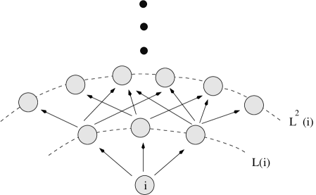
Figure 2: The leaders of an agent $i$ at different levels: ${\mathcal{L}}^{0}(i)=\{i\},{\mathcal{L}}(i),{\mathcal{L}}^{2}(i),\cdots$.

Theorem 3 (Positivity)

Suppose $\eta_{i}^{0}\geq 0$ for $i=1,\dots,k$. Then for all $t>0$ and $i$, $\eta_{i}(t)\geq 0$.

Proof. For any agent $i$ in the flock, define

$$\begin{split}{\mathcal{L}}^{0}(i)&=\{i\},\\ {\mathcal{L}}^{m}(i)&={\mathcal{L}}({\mathcal{L}}^{m-1}(i)),\qquad\mbox{all $m$-th level leaders of $i$},\quad\mbox{and}\\ [{\mathcal{L}}](i)&={\mathcal{L}}^{0}(i)\cup{\mathcal{L}}^{1}(i)\cup{\mathcal{L}}^{2}(i)\cdots,\qquad\mbox{all leaders of $i$, direct or indirect}.\end{split}$$ (21)

Then it is easy to see that the system (20) restricted on $[{\mathcal{L}}](i)$ is always self-contained, i.e., $(\eta_{j}\mid j\in[{\mathcal{L}}](i))$ is not influenced by any variables in $(\eta_{j}\mid j\notin[{\mathcal{L}}](i))$ (but certainly not vice versa).

For convenience, we shall call the restriction of the system (19) or (20) on the sub-flock $[{\mathcal{L}}](i)$ the $[{\mathcal{L}}](i)$-system. Then it suffices to establish the theorem for each $[{\mathcal{L}}](i)$ system. In Figure 2, we have sketched an example of the hierarchies of leaders of a given agent $i$.

Suppose otherwise that the theorem were false on an $[{\mathcal{L}}](i)$-system for some particular agent $i$. There would exist some $\bar{j}\in[{\mathcal{L}}](i)$, and $\bar{t}>0$ such that $\eta_{\bar{j}}(\bar{t})<0$. Define

$$t_{\ast}=\inf\{t>0\mid\mbox{there exists some}\;j\in[{\mathcal{L}}](i),\;\mbox{such that}\;\eta_{j}(t)<0\}.$$

Then $0\leq t_{\ast}\leq\bar{t}<\infty$, and we claim additionally the following.

1. For any $j\in[{\mathcal{L}}](i)$, $\eta_{j}(t_{\ast})\geq 0$.

2. There must exist some $\hat{j}\in[{\mathcal{L}}](i)$, and a sequence of moments $(t_{n})$ such that $t_{n}>t_{\ast}$, $t_{n}\to t_{\ast}$ as $n\to\infty$, and $\eta_{\hat{j}}(t_{n})<0$.

3. There must exist some $j_{\ast}\in[{\mathcal{L}}](i)$, such that $\eta_{j_{\ast}}(t_{\ast})>0$.

(i) and (ii) result directly from the definition of $t_{\ast}$. Suppose otherwise (iii) were false. Then in particular, for any $j\in[{\mathcal{L}}](\hat{j})$, one must have $\eta_{j}(t_{\ast})=0$ by (i). Consider the $[{\mathcal{L}}](\hat{j})$-system after $t_{\ast}$:

$$\dot{\eta}_{j}=\sum_{l\in{\mathcal{L}}(j)}a_{jl}(t)(\eta_{l}-\eta_{j}),\qquad j\in[{\mathcal{L}}](\hat{j}),\;\;t>t_{\ast}.$$

Since this is a homogeneous system with zero initial conditions at $t=t_{\ast}$, by the uniqueness theorem of ODEs (e.g., [10]), the solution to the $[{\mathcal{L}}](\hat{j})$-system must be identically zero: $\eta_{j}(t)\equiv 0$ for any $t>t_{\ast}$ and $j\in[{\mathcal{L}}](\hat{j})$. Now that $\hat{j}\in[{\mathcal{L}}](\hat{j})$, one must have $\eta_{\hat{j}}(t)\equiv 0$ for all $t>t_{\ast}$, which contradicts to Property (ii). Thus (iii) holds.

Define

$$\hat{m}=\min\{m\geq 0\mid\mbox{there exists some $j_{\ast}\in{\mathcal{L}}^{m}(i)$, such that}\;\eta_{j_{\ast}}(t_{\ast})>0\}.$$

Property (i) and (iii) imply that $0<\hat{m}<\infty$. Then by iteratively differentiating the ${\mathcal{L}}(\hat{j})$-system, one can easily establish:

$$\eta_{\hat{j}}(t_{\ast})=\eta^{\prime}_{\hat{j}}(t_{\ast})=\cdots=\eta^{(\hat{m}-1)}_{\hat{j}}(t_{\ast})=0,\qquad\eta^{(\hat{m})}_{\hat{j}}(t_{\ast})>0,$$

which contradicts to Property (ii). Thus the theorem must hold and the proof is complete. $\blacksquare$

The most important consequence is the following bounding capability.

Theorem 4 (Boundedness of Velocities under Evolution)

The Cucker-Smale model (18) has the following closedness properties.

1. Suppose $\Omega$ is a convex compact domain in ${\mathbb{R}}^{3}$, and for any agent $i$, initially $v_{i}(t=0)\in\Omega$. Then for any $t>0$ and $i$, $v_{i}(t)\in\Omega$.

2. In particular, let $D_{0}=\max_{i}|v_{i}(t=0)|$. Then $|v_{i}(t)|\leq D_{0}$ for all $t>0$ and $i$.

Proof. Since the closed ball $B_{D_{0}}(0)$ in ${\mathbb{R}}^{3}$ is convex and compact, (ii) is implied by (i). It suffices to establish (i).

For any unit vector $n\in S^{2}$, and given vector $a\in{\mathbb{R}}^{3}$. We first claim that if

$$n\cdot(v_{i}-a)\big{|}_{t=0}\geq 0,\qquad\forall\;i,$$

then $n\cdot(v_{i}(t)-a)\geq 0$ remains valid for all $t>0$ and $i$. To proceed, define $\eta_{i}=n\cdot(v_{i}-a)$.

$$\begin{split}\dot{\eta}&=n\cdot\dot{v}_{i}\\ &=n\cdot\left(\sum_{j\in{\mathcal{L}}(i)}a_{ij}(t)(v_{j}-v_{i})\right)\\ &=n\cdot\left(\sum_{j\in{\mathcal{L}}(i)}a_{ij}(t)\left[(v_{j}-a)-(v_{i}-a)\right]\right)\\ &=\sum_{j\in{\mathcal{L}}(i)}a_{ij}(t)(\eta_{j}-\eta_{i})\\ &=-(L_{t}\eta)_{i}.\end{split}$$

Then by the preceding theorem, the claim is indeed valid: $\eta_{i}(t)\geq 0$ for all $t>0$ and $i$.

For any compact convex domain $\Omega$, let $p:S^{2}\to{\mathbb{R}}^{3}$ be its support function, so that for any unit direction $n\in S^{2}$, $a=p(n)$ has the property that $a\in\partial\Omega$ and the closed flat half-space

$$\pi_{a,-n}=\{x\in{\mathbb{R}}^{3}\mid(-n)\cdot(x-a)\geq 0\}$$

contains $\Omega$. When the domain is convex but not strictly convex, $p(n)$ could be a set of points, which however does not influence the argument herein. Furthermore, we have

$$\Omega=\bigcap_{n\in S^{2}}\pi_{p(n),-n}.$$

Since each half-space has just been shown invariant under the Cucker-Smale evolution, we conclude that $\Omega$ must be invariant as well under the evolution, which completes the proof. $\blacksquare$

4.2 Perturbation and Induction

We now first prepare a lemma. Together with the boundedness property just established above, it facilitates the later analysis on the emergent behavior of HL flocks.

Lemma 3

Suppose $x(t),v(t)\in{\mathbb{R}}^{3}$ (which could be considered as $x_{2}-x_{1}$ and $v_{2}-v_{1}$ for a 2-flock), and satisfy the perturbed 2-flock system parametrized by some $T>0$:

$$\begin{cases}\dot{x}=v(t)\\ \dot{v}=-a_{T}(x,t)v(t)+\varepsilon_{T}(t),\qquad t\geq 0.\end{cases}$$ (22)

Assume in addition that the following conditions hold.

1. $\displaystyle a_{T}(x,t)\geq\frac{H}{(1+|x|^{2})^{\beta}}$, with $\beta<1/2$.

2. $\varepsilon_{T}\in{\mathbb{R}}^{3}$, and

   $$\left|\varepsilon_{T}(t)\right|\leq ae^{-b(t+T)^{\eta}},\qquad\mbox{for some $\eta\in(0,1]$}.$$ (23)

3. $|v(t)|\leq D_{0}$ for all $t\geq 0$, and $|x_{0}|\leq R_{0}+D_{0}T$.

Here $H,\beta,a,b,\eta,D_{0}$, and $R_{0}$ are given constants independent of $T$. Let $(x^{T}(t),v^{T}(t))$ denote the dependency on $T$. Then

$$|v^{T}(T)|\leq Ae^{-BT^{(1-2\beta)\wedge\eta^{-}}},$$ (24)

where $\eta^{-}=\eta-\delta$ for any small but positive $\delta$ when $\eta<1$, and $\eta^{-}=1$ when $\eta=1$, and $A$ and $B$ are two constants only depending upon $H,\beta,a,b,\eta^{-},D_{0}$, and $R_{0}$ (but not $T$). The notation $a\wedge b$ represents $\min(a,b)$.

Remark 1

We first make two comments on the conditions.

1. The all-time bound $|v(t)|\leq D_{0}$ seems very stringent, but is now natural by Theorem 4 in the preceding subsection.

2. As outlined in the beginning of the current section, the lemma will be applied during the induction process going from the sub-flock $[1,\dots,i-1]$ to $[1,\dots,i]$. To agent $i$, the perturbation factor $\varepsilon_{T}(t)$ comes from the exponentially small dispersion of the leading sub-flock $[1,\dots,i-1]$ from reaching exact emergence.

We now proceed to the proof of Lemma 3.

Proof. From the equation for $v$, we have

$$\begin{split}\langle v,\;\dot{v}\rangle&=-a_{T}(x,t)\langle v,\;v\rangle+\langle v,\;\varepsilon_{T}(t)\rangle,\qquad\mbox{or}\\ |v|\cdot|v|_{t}=\frac{1}{2}\left(|v|^{2}\right)_{t}&=-a_{T}|v|^{2}+\langle v,\;\varepsilon_{T}(t)\rangle.\end{split}$$

Assuming that $v$ is never identically zero on any non-empty open time interval (noticing that the opposite scenario trivializes the lemma on any such intervals and the following argument only needs a minor modification), one has

$$\begin{split}|v|_{t}&\leq-a_{T}|v|+|\varepsilon_{T}|\\ &\leq-\frac{H}{(1+|x|^{2})^{\beta}}|v|+ae^{-b(t+T)^{\eta}},\end{split}$$

by the conditions (i) and (ii). By $\dot{x}=v$ and (iii),

$$\begin{split}|x|&\leq|x_{0}|+\int_{0}^{t}|v|(\tau)d\tau\\ &\leq R_{0}+D_{0}T+D_{0}t=R_{0}+D_{0}(t+T).\end{split}$$

As a result,

$$|v|_{t}\leq-\frac{H}{\left(1+(R_{0}+D_{0}(t+T))^{2}\right)^{\beta}}|v|+ae^{-b(t+T)^{\eta}}.$$

Then by the Gronwall-type integration,

$$\begin{split}|v(t)|&\leq|v_{0}|e^{-\int_{0}^{t}\frac{H}{\left(1+(R_{0}+D_{0}(\tau+T))^{2}\right)^{\beta}}d\tau}+a\int_{0}^{t}e^{-b(\tau+T)^{\eta}}\cdot e^{-\int_{\tau}^{t}\frac{H}{\left(1+(R_{0}+D_{0}(s+T))^{2}\right)^{\beta}}ds}d\tau\\ &\leq D_{0}\cdot e^{-\frac{Ht}{\left(1+(R_{0}+D_{0}(t+T))^{2}\right)^{\beta}}}+\frac{a}{b\eta}T^{1-\eta}e^{-bT^{\eta}}.\end{split}$$

We denote $v(t)$ by $v^{T}(t)$ to indicate its dependency on $T$. Then

$$\begin{split}|v^{T}(T)|&\leq D_{0}\cdot e^{-\frac{H\cdot T}{\left(1+(R_{0}+2D_{0}T)^{2}\right)^{\beta}}}+\frac{\tilde{a}(a,b,\eta^{-})}{b\eta^{-}}e^{-bT^{\eta^{-}}}\\ &\leq D_{0}e^{-\tilde{H}(H,R_{0},D_{0},\beta)T^{1-2\beta}}+C(a,b,\eta^{-})e^{-bT^{\eta^{-}}}\qquad\mbox{(when $T\geq 1$)}\\ &\leq Ae^{-BT^{(1-2\beta)\wedge\eta^{-}}},\end{split}$$

where the two constants $A$ and $B$ are independent of $T$. Also notice that when $\eta=1$, the monomial factor $T^{1-\eta}=1$ and the lowering from $\eta$ to $\eta^{-}$ is unnecessary in the first line. Finally, since $|v^{T}(t)|\leq D_{0}$ by the given conditions, by suitably increasing $A$, the condition $T\geq 1$ in the last second line can actually be removed. This completes the proof. $\blacksquare$

We are now ready to state and prove the main theorem.

Theorem 5 (Convergence of an HL Flock)

Let $[1,2,\dots,k]$ be a Cucker-Smale flock under hierarchical leadership with $\beta<1/2$. Then for some $B>0$, which depends only on the initial configuration and all the system parameters, one has

$$\max_{1\leq i,j\leq k}|v_{i}(t)-v_{j}(t)|=O(e^{-Bt}),\qquad t>0.$$ (25)

Proof. We prove the theorem by induction on the sub-flocks, from $[1,\dots,l-1]$ to $[1,\dots,l]$.

First we show that the theorem holds for a 2-flock $[1,2]$. By definition, the leader set ${\mathcal{L}}(2)$ is nonempty and has to be ${\mathcal{L}}(2)=\{1\}$, i.e., $a_{21}>0$. Let $x=x_{2}-x_{1}$, and $v=v_{2}-v_{1}$. Then

$$\begin{cases}\dot{x}=v\\ \dot{v}=\dot{v}_{2}-\dot{v}_{1}=\dot{v}_{2}=a_{21}(v_{1}-v_{2})=-a_{21}v.\end{cases}$$

Here $\displaystyle a_{21}=a_{21}(x)=\frac{H}{(1+|x|^{2})^{\beta}}$, with $\beta<1/2$. Then Cucker and Smale’s analysis in [4] still applies directly, and $|v(t)|=O(e^{-Bt})$ for some $B>0$.

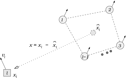
Figure 3: The induction process from $[1,\dots,l-1]$ to $[1,\dots,l-1,l]$ reduces the $l$-flock system to a perturbed 2-flock system.

Assume now that the theorem holds for the sub-flock $[1,\dots,l-1]$, we intend to show that it must be true for $[1,\dots,l-1,l]$ as well for $l>2$. As a result, the main focus shall be the agent $l$.

By induction, there exists some $b>0$, such that

$$\max_{i,j\in\{1,\dots,l-1\}}|v_{i}(t)-v_{j}(t)|=O(e^{-bt}),\qquad t\to\infty.$$ (26)

Define the average velocity (of the direct leaders of agent $l$) by

$$\hat{v}_{l}(t)=\frac{1}{d}_{l}\sum_{i\in{\mathcal{L}}(l)}v_{i}(t),\qquad\mbox{with}\;d_{l}=\#{\mathcal{L}}[l].$$

Then for any $j\in{\mathcal{L}}(l)$,

$$|v_{j}(t)-\hat{v}_{l}(t)|\leq\frac{1}{d_{l}}\sum_{i\in{\mathcal{L}}(l)}|v_{j}-v_{i}|=O(e^{-bt}),$$ (27)

by the induction assumption. Similarly, define

$$\hat{x}_{l}(t)=\frac{1}{d_{l}}\sum_{i\in{\mathcal{L}}(l)}x_{i}(t),\quad\mbox{and}\quad x(t)=x_{l}(t)-\hat{x}_{l}(t),\quad v(t)=v_{l}(t)-\hat{v}_{l}(t).$$

Then $\dot{x}=v$, and

$$\begin{split}\dot{v}&=\dot{v}_{l}-\frac{d\hat{v}_{l}}{dt}=\sum_{j\in{\mathcal{L}}(l)}a_{lj}\cdot(v_{j}-v_{l})-\frac{d\hat{v}_{l}}{dt}\\ &=\sum_{j\in{\mathcal{L}}(l)}a_{lj}\cdot(\hat{v}_{l}-v_{l})+\underbrace{\sum_{j\in{\mathcal{L}}(l)}a_{lj}\cdot(v_{j}-\hat{v}_{l})-\frac{d\hat{v}_{l}}{dt}}_{\varepsilon(t)}.\end{split}$$ (28)

Since each $\dot{v}_{i}$ ($i\in{\mathcal{L}}(l)$) is the linear combination of some $(v_{j}-v_{i})$’s with $j\in{\mathcal{L}}(i)\subseteq\{1,\dots,l-1\}$, by (26), one must have

$$\frac{d\hat{v}_{l}}{dt}=O(e^{-bt}).$$

Similarly, due to (27) and the boundedness of $a_{lj}$’s, one has

$$\big{|}\sum_{j\in{\mathcal{L}}(l)}a_{lj}\cdot(v_{j}-\hat{v}_{l})\big{|}=O(e^{-bt}).$$

In combination, we conclude that

$$|\varepsilon(t)|\leq ce^{-bt},\qquad t>0,\quad\mbox{for some}\;c>0.$$ (29)

On the other hand, define

$$a=\sum_{j\in{\mathcal{L}}(l)}a_{lj}=\sum_{j\in{\mathcal{L}}(l)}\frac{H}{\left(1+|x_{j}-x_{l}|^{2}\right)^{\beta}}.$$ (30)

Then (28) simply becomes

$$\dot{v}=-av+\varepsilon.$$ (31)

Define $\displaystyle g(s)=\frac{H}{(1+s)^{\beta}}$ with $s\geq 0$. Then $g(s)$ is convex, and

$$\frac{1}{d_{l}}\sum_{j\in{\mathcal{L}}(l)}g(s_{j})\geq g\left(\frac{1}{d_{l}}\sum_{j\in{\mathcal{L}}(l)}s_{j}\right).$$

As a result, when $s_{j}=|x_{j}-x_{l}|$,

$$\sum_{j\in{\mathcal{L}}(l)}\frac{H}{(1+|x_{j}-x_{l}|^{2})^{\beta}}\geq d_{l}\frac{H}{\left(1+\frac{1}{d_{l}}\sum_{j\in{\mathcal{L}}(l)}|x_{j}-x_{l}|^{2}\right)^{\beta}}.$$ (32)

By the least-square principle,

$$\frac{1}{d_{l}}\sum_{j\in{\mathcal{L}}(l)}|x_{l}-x_{j}|^{2}=|\overbrace{x_{l}-\hat{x}_{l}}^{x}|^{2}+\frac{1}{d_{l}}\sum_{j\in{\mathcal{L}}(l)}|x_{j}-\hat{x}_{l}|^{2},$$ (33)

since $\hat{x}_{l}$ is the center or mean of $\{x_{j}\mid j\in{\mathcal{L}}(l)\}$. By the induction assumption on the emergence of $[1,\dots,l-1]\supseteq{\mathcal{L}}(l)$, there exists some $M>0$, such that

$$\frac{1}{d_{l}}\sum_{j\in{\mathcal{L}}(l)}|x_{j}-\hat{x}_{l}|^{2}\leq M-1.$$ (34)

Combining Eqn.’s (30) through (34), we have

$$a=a(x,t)\geq\frac{d_{l}H}{(M+|x|^{2})^{\beta}}\geq\frac{\tilde{H}}{(1+|x|^{2})^{\beta}},$$ (35)

where the updated constant $\tilde{H}=\tilde{H}(H,d_{l},M,\beta)$. (Notice that the notation $a(x,t)$ summarizes all the influence from $\{x_{j}\mid j\in{\mathcal{L}}(l)\}$ into the $t$-variable.)

The combination of (29), (31), and (35) leads to the reduced system:

$$\begin{cases}\dot{x}=v\\ \dot{v}=-a(x,t)v+\varepsilon(t),\end{cases}$$ (36)

with $\displaystyle a(x,t)\geq\frac{\tilde{H}}{(1+|x|)^{\beta}},\quad\mbox{and}\quad|\varepsilon(t)|\leq ce^{-bt}$. In order to apply Lemma 3, further define

$$D_{0}=2\max_{1\leq i\leq k}|v_{i}(t=0)|,\quad\mbox{and}\quad R_{0}=2\max_{1\leq i\leq k}|x_{i}(t=0)|.$$ (37)

Then by Theorem 4, we have

$$|v_{i}(t)|\leq\frac{D_{0}}{2},\qquad\forall\;i\;\mbox{and}\;t>0.$$

Consequently,

$$|v(t)|\leq\frac{1}{d_{l}}\sum_{j\in{\mathcal{L}}(l)}|v_{j}-v_{l}|\leq\frac{1}{d_{l}}\sum_{j\in{\mathcal{L}}(l)}D_{0}=D_{0}.$$ (38)

Similarly, for any $T>0$,

$$\begin{split}|x(T)-x(0)|&\leq|x_{l}(T)-x_{l}(0)|+\frac{1}{d_{l}}\sum_{j\in{\mathcal{L}}(l)}|x_{j}(T)-x_{j}(0)|\\ &\leq\frac{D_{0}}{2}T+\frac{1}{d}_{l}\sum_{j\in{\mathcal{L}}(l)}\frac{D_{0}}{2}T=D_{0}T.\end{split}$$

As a result,

$$\begin{split}|x(T)|&\leq|x(0)|+D_{0}T\\ &\leq|x_{l}(0)|+\frac{1}{d_{l}}\sum_{j\in{\mathcal{L}}(l)}|x_{j}(0)|+D_{0}T\\ &\leq\frac{R_{0}}{2}+\frac{1}{d_{l}}\sum_{j\in{\mathcal{L}}(l)}\frac{R_{0}}{2}+D_{0}T=R_{0}+D_{0}T.\end{split}$$ (39)

To conclude, for any $T>0$, if we define

$$x^{T}(t)=x(t+T),\quad v^{T}(t)=v(t+T),\quad a_{T}(x^{T},t)=a(x^{T},t+T),\;\;\mbox{and}\;\;\varepsilon_{T}(t)=\varepsilon(t+T),$$

then,

$$\begin{cases}\dot{x}^{T}=v^{T}\\ \dot{v}^{T}=-a_{T}(x^{T},t)v^{T}+\varepsilon_{T}(t),\qquad t>0,\end{cases}$$

and all the three conditions in Lemma 3 are satisfied (with $\eta=1$). Therefore, there must exist two positive constants $\tilde{A}$ and $\tilde{B}$, such that for any $T>0$,

$$|v(2T)|=|v^{T}(T)|\leq\tilde{A}e^{-\tilde{B}T^{(1-2\beta)\wedge 1}}=\tilde{A}e^{-\tilde{B}T^{1-2\beta}}.$$

Since $T$ is arbitrary, we thus must have, after adjusting the constants,

$$|v(t)|\leq\hat{A}e^{-\hat{B}t^{1-2\beta}},\qquad t>0,\qquad\mbox{for some constants $\hat{A}$ and $\hat{B}$}.$$

Moreover, since $\beta<1/2$ by assumption, one then must have

$$\int_{0}^{\infty}|v(t)|dt<\infty,$$

which in return implies that there exists some constant $M>0$, such that

$$|x(t)|\leq M,\qquad t>0.$$

Then by repeating the similar calculation in the proof of Lemma 3, assisted with this new constant bound $|x|\leq M$ instead of $|x|\leq R_{0}+D_{0}(t+T)$ there, one arrives at:

$$|v(t)|\leq A^{\prime}e^{-B^{\prime}t},\qquad\mbox{(since $\eta=1$),}$$

for two positive constants $A^{\prime}$ and $B^{\prime}$ independent of $t$. Combined with the induction base (26), we thus conclude that the theorem must hold true for the sub-flock $[1,\dots,l-1,l]$ with the exponent coefficient $B=B^{\prime}\wedge b$. This completes the proof. $\blacksquare$

5 HL Flocking Under a Free-Will Leader

In this section, partially inspired by the preceding perturbation methods, we investigate a more realistic scenario when the ultimate leader agent 0 (in an HL flock $[0,1,\dots,k]$) can have a free-will acceleration, instead of merely flying in a constant velocity.

The following phenomenon is not uncommon near lakes, grasslands, or any open spaces where a flock of birds often visit. When the flock is initially approached by an unexpected pedestrian or a predator from a corner on the outer rim, the bird which takes off first (and alerts others subsequently) generally takes a curvy flying path before it reaches a stable flying pattern with an almost constant velocity. Such a bird gains the full speed fast, flies ahead of the entire flock, and serves as a virtual overall leader.

For an HL flock $[0,1,\dots,k]$, in addition to the Cucker-Smale system

$$\begin{cases}\dot{x}_{i}=v_{i}(t)\\ \dot{v}_{i}=\sum_{j\in{\mathcal{L}}(i)}a_{ij}(x)(v_{j}(t)-v_{i}(t)),\qquad i>0,\end{cases}$$ (40)

we now also impose for the ultimate leader agent 0:

$$\begin{cases}\dot{x}_{0}=v_{0}\\ \dot{v}_{0}=f(t),\qquad t>0,\end{cases}$$ (41)

coupled with a given set of initial conditions. For convenience, we shall call $f(t)$ the free-will acceleration  of the leader. In combination, the new system is no longer autonomous.

The main goal of this section is to establish the following theorem.

Theorem 6

Suppose an HL (k+1)-flock $[0,\dots,k]$ with a free-will leader satisfies both (40) and (41), with the Cucker-Smale connectivity strength of $\beta<1/2$. In addition, assume that the leader’s free-will acceleration satisfies

$$|f(t)|=O((1+t)^{-\mu}),\qquad\mbox{with some exponent $\mu>k$.}$$

Then the flock still has the following emergent behavior:

$$\max_{0\leq i,j\leq k}|v_{i}-v_{j}|(t)=O\left((1+t)^{-(\mu-k)}\right).$$

Remark 2

We first make two comments regarding why one should expect to put some regularity conditions on the leader’s behavior in order for a coherent pattern to emerge asymptotically.

1. Intuitively, if the leader keeps changing its velocity substantially, it will be more difficult for the entire flock to follow and behave coherently. An extreme example is a flock with a drunken leader which flies in a Brownian random path. Then the entire flock cannot be expected to synchronize with the unpredictable motion of the leader instantaneously.

2. In the theorem, the decaying constraint $\mu>k$ depends on the size $k$ of the flock. Thus qualitatively speaking, it requires the leader to exert less free will when the flock is larger, in order to lead a coherent flock asymptotically. Consider the special hierarchical leadership under a linear chain of command:

   $$k\to k-1\to\cdots\to 1\to 0.$$

   The tail agent $k$ has to go through all the $k$ intermediate stages to sense any move that the leader is making. Thus intuitively, there will be a long time delay in between, and the leader has to be tempered enough to allow its distantly connected followers to respond coherently.

We first prepare a lemma that is similar to Lemma 3. Since the new non-autonomous system does not necessarily have the positivity property, we take a slightly different approach.

Lemma 4

Let $x,v,g\in{\mathbb{R}}^{3}$, and satisfy

$$\begin{cases}\dot{x}=v(t)\\ \dot{v}=-a(x,t)v(t)+g(t).\end{cases}$$

Suppose that

$$\begin{split}a(x,t)&\geq\frac{H}{(1+|x|^{2})^{\beta}},\qquad\mbox{for some $\beta<1/2$, and},\\ |g(t)|&=O\left((1+t)^{-\eta}\right),\qquad\mbox{with some constant $\eta>1$}.\end{split}$$

Then, $|v(t)|=O((1+t)^{-(\eta-1)})$ with the order constant only depending on the initial conditions $x(t=0),v(t=0)$, and $H$, $\beta$, and $\eta$.

Proof. From the second equation, one has

$$|v|\cdot|v|_{t}=\left(\frac{v^{2}}{2}\right)_{t}=\langle v,\;v_{t}\rangle=-a\langle v,\;v\rangle+\langle v,\;g\rangle\leq-a|v|^{2}+|v|\cdot|g|$$

Assume that $v$ does not vanish identically on any non-empty open intervals for the same reason as in the proof of Lemma 3. Then one has

$$|v|_{t}\leq-a|v|+|g|,\qquad t>0.$$

Fix any time $T>0$, and define

$$|x|_{\ast}=\sup_{t\leq T}|x|(t),\quad\mbox{and}\quad a_{\ast}=\inf_{t\leq T}\frac{H}{(1+|x|^{2})^{\beta}}=\frac{H}{(1+|x|^{2}_{\ast})^{\beta}.}$$ (42)

Then one has

$$|v|_{t}\leq-a_{\ast}|v|+|g|,\qquad t\in[0,T].$$ (43)

Since $a_{\ast}$ is constant, integration yields

$$|v|(t)\leq|v|(0)e^{-a_{\ast}t}+\int_{0}^{t}|g|(\tau)e^{-a_{\ast}(t-\tau)}d\tau.$$

In particular, for any $t<T$,

$$|v|(t)\leq|v|(0)+\int_{0}^{t}|g|(\tau)d\tau\leq|v|(0)+\int_{0}^{\infty}|g(\tau)|d\tau:=A_{0}.$$

(Since $\eta>1$ by assumption, the integral of $|g|$ is finite.) Now that $A_{0}$ is independent of the time mark $T$, we conclude that the last upper bound must hold for any $t>0$: $|v|(t)\leq A_{0},t>0$. Therefore, from the first equation $\dot{x}=v(t)$, one has

$$|x|(t)\leq|x|(0)+\int_{0}^{t}|v|(\tau)d\tau\leq B_{0}+A_{0}t,\quad t>0,$$

where $B_{0}=|x|(0)$. In particular, for any time mark $T>0$, the quantities in (42) are subject to:

$$|x|_{\ast}\leq B_{0}+A_{0}T,\quad\mbox{and}\quad a_{\ast}\geq\frac{H}{[1+(B_{0}+A_{0}T)^{2}]^{\beta}}.$$

We then go back and integrate the inequality (43) again, but from $T/2$ to $T$ this time:

$$\begin{split}|v|(T)&\leq|v|(T/2)e^{-\frac{a_{\ast}T}{2}}+\int_{T/2}^{T}|g|(\tau)e^{-a_{\ast}(T-t)}dt\\ &\leq A_{0}e^{-\frac{HT/2}{[1+(B_{0}+A_{0}T)^{2}]^{\beta}}}+\int_{T/2}^{\infty}|g|(t)dt\\ &\leq A_{0}e^{-\tilde{H}(A_{0},B_{0},\beta)(1+T)^{1-2\beta}}+\int_{T/2}^{\infty}O\left((1+t)^{-\mu}\right)dt\\ &=A_{0}e^{-\tilde{H}(1+T)^{1-2\beta}}+O\left((1+T)^{-(\mu-1)}\right).\end{split}$$

Since $\beta<1/2$, we conclude that

$$|v|(T)=O\left((1+T)^{-(\mu-1)}\right),$$

where the constant in $O(\cdot)$ is independent of $T$. Since $T$ is arbitrary, the lemma is established. $\blacksquare$

We are now ready to prove Theorem 6. Details on some similar calculations will be directed to the proof of Theorem 5.

Proof. It suffices to prove the following more general result:

$$\max_{0\leq i,j\leq l}|v_{i}-v_{j}|(t)=O\left((1+t)^{-(\mu-l)}\right),\qquad t>0,$$ (44)

for any sub-flock $[0,1,\dots,l]$ and $l\geq 1$.

When $l=1$, define $x=x_{1}-x_{0}$ and $v=v_{1}-v_{0}$. Then $\dot{x}=v$, and

$$\dot{v}=\dot{v}_{1}-\dot{v}_{0}=a_{10}(v_{0}-v_{1})-f=-a_{10}v-f.$$

By the definition of an HL flock, ${\mathcal{L}}(1)\neq\varnothing$, and it has to be agent $0$, implying that $a_{10}$ is subject to the Cucker-Smale formula. Then by the preceding lemma (with $\eta=\mu$), one has

$$|v|(t)=O\left((1+t)^{-(\mu-1)}\right),$$

and (44) holds.

Suppose now that (44) is true for the sub-flock $[0,1,\dots,l-1]$ with $2\leq l\leq k$, so that

$$\max_{0\leq i,j\leq l-1}|v_{i}-v_{j}|(t)=O\left((1+t)^{-(\mu-l+1)}\right).$$ (45)

As in the proof of Theorem 5, define the average features of the direct leaders of agent $l$ by:

$$\hat{x}_{l}=\frac{1}{d_{l}}\sum_{j\in{\mathcal{L}}(l)}x_{j},\quad\mbox{and}\quad\hat{v}_{l}=\frac{1}{d_{l}}\sum_{j\in{\mathcal{L}}(l)}v_{j},\qquad d_{l}=\#{\mathcal{L}}(l),$$

and $x=x_{l}-\hat{x}_{l}$ and $v=v_{l}-\hat{v}_{l}$.

Then as in the proof of Theorem 5, one has $\dot{x}=v$ and

$$\begin{split}\dot{v}&=-a(x,t)\cdot v+g_{l}(t),\qquad\mbox{with}\\ g_{l}(t)&=\sum_{j\in{\mathcal{L}}(l)}a_{lj}\cdot(v_{j}-\hat{v}_{l})-\frac{d\hat{v}_{l}}{dt}.\\ a(x,t)&=\sum_{j\in{\mathcal{L}}(l)}a_{lj}(x_{l}-x_{j}).\end{split}$$

We first estimate $g_{l}$. Since $|a_{lj}|\leq H$ and ${\mathcal{L}}(l)\subseteq[0,1,\dots,l-1]$, by the induction assumption (45), the first term in $g_{l}$ must be of the order $O((1+t)^{-\eta})$ with $\eta=\mu-l+1$. For the remaining second term in $g_{l}$, let $\displaystyle 1_{0\in{\mathcal{L}}(l)}$ denote the logical variable which is 1 when agent 0 belongs to ${\mathcal{L}}(l)$, and 0 otherwise. Then

$$\frac{d\hat{v}_{l}}{dt}=\frac{1}{d_{l}}\sum_{j\in{\mathcal{L}}(l)}\dot{v}_{j}=1_{0\in{\mathcal{L}}(l)}\cdot\frac{1}{d_{l}}\dot{v}_{0}+\frac{1}{d_{l}}\sum_{j\in{\mathcal{L}}(l)\setminus\{0\}}\dot{v}_{j}.$$

Now that $\dot{v}_{0}=f(t)=O((1+t)^{-\mu})$, and each $\dot{v}_{j}$ with $j\in{\mathcal{L}}(l)\setminus\{0\}$ is some linear combination of $(v_{s}-v_{j})$ with $s$’s in ${\mathcal{L}}(j)\subseteq[0,1,\dots,l-1]$. Thus by the induction assumption (45), one must have $\frac{d\hat{v}_{l}}{dt}=O((1+t)^{-\eta})$ with $\eta=\mu-l+1$.

We now estimate $a(x,t)$. Since $\mu>k$ by the given condition, we have $\mu-l+1>k-l+1=1$. As a result, by the induction assumption on the sub-flock $[0,1,\dots,l-1]$, for any $i,j\leq l-1$,

$$\begin{split}|x_{i}-x_{j}|(t)&\leq|x_{i}-x_{j}|(0)+\int_{0}^{t}|v_{i}-v_{j}|(\tau)d\tau\\ &\leq|x_{i}-x_{j}|(0)+\int_{0}^{\infty}O\left((1+\tau)^{-(\mu-l+1)}\right)d\tau<\infty,\qquad\forall\;t>0.\end{split}$$

Therefore the boundedness property in (34) still holds, and the same calculation in the proof of Theorem 5 leads to

$$a(x,t)\geq\frac{\tilde{H}}{(1+|x|^{2})^{\beta}},$$

for some constant $\tilde{H}=\tilde{H}(H,d_{l},\beta,f,\mbox{initial conditions of}\;[0,\dots,l-1])$.

Combining the estimations on $g_{l}$ and $a$, one sees that $x(t)$ and $v(t)$ satisfy a perturbed system as in Lemma 4 with $\eta=\mu-l+1$. Therefore, by Lemma 4,

$$|v_{l}-\hat{v}_{l}|(t)=|v|(t)=O\left((1+t)^{-(\eta-1)}\right)=O\left((1+t)^{-(\mu-l)}\right).$$

Now that by the induction assumption, for any $j\leq l-1$, one must have

$$|v_{j}-\hat{v}_{l}|(t)=O\left((1+t)^{-(\mu-l+1)}\right),\;\;\mbox{since}\;|v_{j}-v_{i}|=O\left((1+t)^{-(\mu-l+1)}\right),\;\;\forall\;i\in{\mathcal{L}}(l).$$

Therefore, for any $j\leq l-1$,

$$|v_{l}-v_{j}|\leq|v_{l}-\hat{v}_{l}|+|v_{j}-\hat{v}_{l}|=O\left((1+t)^{-(\mu-l)}\right).$$

This completes the proof of (45), and thus the entire theorem. $\blacksquare$

Corollary 2

Under the same statements as in the preceding theorem, suppose $\mu>k+1$, then there exists a constant configuration $\displaystyle(d_{ij})_{0\leq i,j\leq k}$ with $d_{ij}\in{\mathbb{R}}^{3}$, such that

$$\lim_{t\to\infty}\left(x_{i}(t)-x_{j}(t)\right)=d_{i,j},\qquad 0\leq i,j\leq k,$$

and the convergence rate is $O\left((1+t)^{-(\mu-k-1)}\right)$.

6 Conclusion

In this paper, we have investigated the emergent behavior of Cucker-Smale flocking under the structure of hierarchical leadership  (HL). The convergence rates are established for the general cases of both discrete-time and continuous-time HL flocking, as well as for HL flocking under an overall leader with free-will accelerations.

In all these cases, the consistent convergence towards some asymptotically coherent patterns may reveal the advantages and necessities of having leaders and leadership in a complex (biological, technological, economic, or social) system with sufficient intelligence and memory.

Our future work shall focus more on extending the results herein onto other flocking systems or leadership structures, a few of which have been mentioned in the Introduction.

References

• [1] Y.-L. Chuang, M. R. D’Orsogna, D. Marthaler, A. L. Bertozzi, and L. Chayes. State transitions and the continuum limit for a 2D interacting, self-propelled particle system. submitted to Physica D, 2006.
• [2] F. R. K. Chung. Spectral Graph Theory. AMS, Providence, RI, 1997.
• [3] I. D. Couzin, J. Krause, N. R. Franks, and S. Levin. Effective leadership and decision making in animal groups on the move. Nature, 433:513–516, 2005.
• [4] F. Cucker and S. Smale. Emergent behavior in flocks. IEEE Trans. Automatic Control, to appear, 2006.
• [5] F. Cucker and S. Smale. Lectures on emergence. Preprint, 2006.
• [6] F. Cucker, S. Smale, and D. Zhou. Modeling language evolution. Found. Comput. Math., 4:315–343, 2004.
• [7] I. Daubechies and J. C. Lagarias. Sets of matrices all infinite products of which converge. Linear Alg. Appl., 161:227–263, 1992.
• [8] M. R. D’Orsogna, Y.-L. Chuang, A. L. Bertozzi, and L. Chayes. Self-propelled particles with soft-core interactions: patterns, stability, and collapse. Phys. Rev. Lett., 96(104302), 2006.
• [9] G. Fliel, D. Grünbaum, S. Levin, and D. Olson. From individuals to aggregations: The interplay between behavior and physics. J. Theor. Biol., 196:397–454, 1999.
• [10] M. W. Hirsch, S. Smale, and R. Devaney. Differential Equations, Dynamical Systems, and an Introduction to Chaos. Academic Press, 2 edition, 2003.
• [11] A. Jadbabaie, J. Lin, and A. S. Morse. Coordination of groups of mobile autonomous agents using nearest neighbor rules. IEEE Trans. Automatic Control, 48(6):988–1001, 2003.
• [12] H. Levine and W.-J. Rappel. Self-organization in systems of self-propelled particles. Phys. Rev. E, 63:017101, 2000.
• [13] E. H. Lieb and M. Loss. Analysis. Amer. Math. Soc., second edition, 2001.
• [14] Y. Liu and K. Passino. Stable social foraging swarms in a noisy environment. IEEE Trans. Automatic Control, 49:30–44, 2004.
• [15] J. K. Parrish, S. V. Viscido, and D. Grünbaum. Self-organized fish schools: An examination of emergent properties. Biol. Bull., 202:296–305, 2002.
• [16] G.-C. Rota and G. Strang. A note on the joint spectral radius. Indag. Math., 22:379–381, 1960.
• [17] J. Shen. Compactification of a set of matrices with convergent infinite products. Linear Alg. Appl., 311:177–186, 2000.
• [18] J. Shen. A geometric approach to ergodic non-homogeneous Markov chains. In Wavelet Analysis and Multiresolution Methods, volume 212 of Lecture Note in Pure and Appl. Math., pages 341–366. Marcel Dekker Inc., New York, 2000.
• [19] G. Strang and T. Nguyen. Wavelets and Filter Banks. Wellesley-Cambridge Press, Wellesley, MA, 1996.
• [20] C. M. Topaz and A. L. Bertozzi. Swarming patterns in a two-dimensional kinematic model for biological groups. SIAM J. Appl. Math., 65:152–174, 2004.
• [21] C. M. Topaz, A. L. Bertozzi, and M. A. Lewis. A nonlocal continuum model for biological aggregation. arXiv preprint: q-bio.PE/0504001 v1, 2005.
• [22] J. N. Tsitsiklis, D. P. Bertsekas, and M. Athans. Distributed asynchronous deterministic and stochastic gradient optimization algorithms. IEEE Trans. Automatic Control, AC-31(9).
• [23] T. Vicsek, A. Czirók, E. Ben-Jacob, I. Cohen, and O. Schochet. Novel type of phase transition transition in a system of self-driven particles. Phys. Rev. Lett., 75(6):1226–1229, 1995.