Performance of a new invariants method on homogeneous and non-homogeneous quartet trees

Abstract

An attempt to use phylogenetic invariants for tree reconstruction was made at the end of the 80s and the beginning of the 90s by several authors (the initial idea due to Lake [Lak87] and Cavender and Felsenstein [CF87]). However, the efficiency of methods based on invariants is still in doubt ([Hue95], [JN90]), probably because these methods only used few generators of the set of phylogenetic invariants. The method studied in this paper was first introduced in [CGS05] and it is the first method based on invariants that uses the whole set of generators for DNA data. The simulation studies performed in this paper prove that it is a very competitive and highly efficient phylogenetic reconstruction method, especially for non-homogeneous models on phylogenetic trees.

Introduction

Since the introduction of phylogenetic invariants by Cavender and Felsenstein [CF87], Lake [Lak87] and Evans and Speed [ES93] several attempts to give a generating set of polynomial phylogenetic invariants have been made (see for example [SSEW93], [FS95]) but it has not been until recently that algebraic geometers have managed to find them all [AR04a], [SS05], [CS05]. Methods based on invariants have already proved to be useful in comparative genomics [SB99]). However, a perception seems to have developed that invariants are inefficient, in the technical sense of requiring long sequences to correctly infer a phylogenetic tree, cf. [JN90], [Hue95]. While [Hue95] showed the inefficiency for the use of Lake’s invariants alone, no method using all invariants had been proposed at that point, and the question for invariants-based methods in general was never investigated. Note that Lake’s method of invariants only used two phylogenetic invariants of degree one among the 795 generators of the set of polynomial invariants of a quartet tree for the Kimura 2-parameter model [GP05]. But as Felsenstein explained, invariants are worth more attention for what they might lead to in the future [Fel03]. This future may be soon, since the studies of this paper show a method based on invariants which is indeed promising. Recently, other methods based on a large set of invariants have also been considered [Eri05], [KKPP06].

Phylogenetic invariants are relationships satisfied by the expected pattern frequencies occurring in sequences evolving along a given tree topology $T$ under an evolutionary model. More precisely, if t is the set of $d$ model parameters on $T$ and $p_{\alpha}(\mathbf{t})$ is the probability of observing the pattern $\alpha$ at the leaves of $T$, by letting $\mathbf{t}$ vary on an open subset of $\mathbb{R}^{d}$, the probability vector $p(\mathbf{t})=(p_{AA\dots A}(\mathbf{t}),\dots,p_{TT\dots T}(\mathbf{t}))$ defines a subset $S_{T}$ of dimension $\leq d$ of $\mathbb{R}^{4^{n}}$. A phylogenetic invariant is a real-valued continuous function $f(x)$ on $\mathbb{R}^{4^{n}}$ such that $f(p)=0$ for any $p\in S_{T}$, but not for all the points on the subset $S_{T^{\prime}}$ determined by another tree topology $T^{\prime}$. Essentially, the equations $f(p)=0$ are satisfied for pattern frequencies arising from any model parameters on a fixed tree, so they might be used for recovering the tree topology.

In practice, the vector of observed pattern frequencies $\hat{p}$ obtained from an alignment of sequences for $n$ taxa with enough data, should approximate $p(\mathbf{t})$ for some set of parameters $\mathbf{t}$ on a tree topology $T$. In other words, $\hat{p}$ should be a point close to the subset $S_{T}$ so, if $f$ is an invariant for the topology $T$, one should have that $f(\hat{p})$ is very close to 0. As the tree topology is identifiable via invariant-based methods [AR06], using phylogenetic invariants for tree reconstruction is a consistent method (see [HL00], [Fel03]). A practical introduction to the theory of invariants can be found in the book of J. Felsenstein [Fel03, chapter 22], whereas the book [PS05] provides a beautiful insight into the applications of algebraic statistics (and in particular polynomial phylogenetic invariants) to computational biology.

There are two major motivations for using phylogenetic invariants in tree reconstruction. One of them is the prohibitive computational expense of a full maximum likelihood estimation of a tree, its edge lengths, a base distribution, and a rate matrix. The other is that the evolutionary models underlying the theory of invariants allow for non-homogeneous mutation. Indeed, it is known that, for some biological data sets, different rate matrices should be allowed in different lineages. Thus it is essential to have at our disposal phylogenetic methods for reconstructing trees admitting non-homogeneous models [YY99], [GG98].

In this paper, a phylogenetic reconstruction method that uses polynomial phylogenetic invariants (introduced in [CGS05]) is studied and tested for quartet trees evolving under the Kimura 3-parameter model of nucleotide substitution [Kim81]. Actually, we consider an algebraic Kimura model: the parameters of the model are the entries of the substitution matrices on the edges (and not a single rate matrix together with edge lengths). Hence the model is non-homogenous —because it allows different rate matrices among the edges— but it is stationary (and the distribution of the bases is uniform), and we always assume that all sites are independent and identically distributed (i.i.d. hypotheses). We performed simulation studies to test its efficiency. One of our approaches to evaluate the performance and efficiency of the method is taken from Huelsenbeck [Hue95] so that a large portion of the tree space is examined to get a general idea of how the algorithm performs. We present the results obtained for sequences of length 100 up to 10000.

We also checked the performance of the method on simulated data from non-homogeneous models by carrying out a comparison to Neighbor-Joining algorithm [SN87], maximum likelihood algorithm [Fel81], and an algorithm for a non-homogeneous model from PAML [Yan97] for sequences generated under a Kimura 2-parameter model [Kim80] and different rate matrices along different tree branches.

Results

Homogeneous data

The performance of the invariants method studied here on homogeneous Kimura models can be seen in the figure 1. Using the approach of J.P. Huelsenbeck in [Hue95] for quartet trees, we considered two branch-length parameters $a,b$ and simulated data for each pair of lengths. Parameter $a$ assigns the branch length to the internal branch and two opposite peripheral branches, and parameter $b$ assigns the branch length to the two remaining branches. Parameters $a$ and $b$ were varied from 0.01 to 0.75 in increments of 0.02, and 1000 alignments were simulated for each couple $(a,b)$ (see figures 2 and 3 in [Hue95], or figure I in the Supplementary Material for a clear picture of this space of parameters). The simulated trees evolve under the Kimura 3-parameter model [Kim81] with a fixed rate matrix of the form

$$\,\,A\,\,\,\,C\,\,\,\,G\,\,\,\,T$$

$$\begin{array}[]{c}A\\ C\\ G\\ T\end{array} \left(\begin{array}[]{cccc}\cdot&\gamma&\alpha&\beta\\ \gamma&\cdot&\beta&\alpha\\ \alpha&\beta&\cdot&\gamma\\ \beta&\alpha&\gamma&\cdot\\ \end{array}\right)$$

along the tree ($\cdot=-\alpha-\beta-\gamma$). Figure 1 shows the efficiency of the method considered in this paper for a rate matrix with parameters $\gamma=0.1,\alpha=3.0,\beta=0.5$ (hence, a 5:1 transition:transversion bias) and for nucleotide sequences of lengths 100, 500, 1000 and 10000. See also figures III and IV of the Supplementary Material for studies performed with other rate matrices.

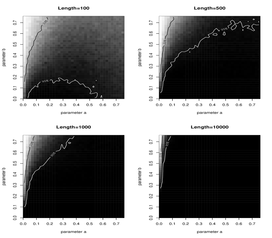
Figure 1: The graphics above represent the probability of reconstructing the correct tree in the parameter space (see Figure I in the Supplementary Material). Black areas correspond to couples $(a,b)$ for which the tree was correctly estimated, while white regions correspond to couples $(a,b)$ for which the tree is never estimated; grey tones indicate areas of intermediate probability. The $95\%$ isocline is drawn in white, while the $33\%$ is drawn in black. The four graphics above show the results obtained under the homogeneous Kimura 3-parameter model when using a rate matrix with parameters $\gamma=0.1,\alpha=3.0,\beta=0.5$ (hence a 5:1 transition:transversion bias).

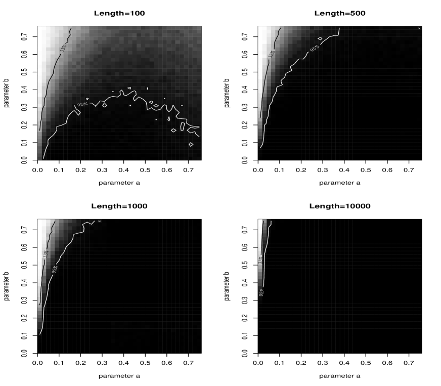
Figure 7: The graphics above represent the probability of reconstructing the correct tree in the parameter space (see Figure I). Black areas correspond to couples $(a,b)$ for which the tree was correctly estimated, while white regions correspond to couples $(a,b)$ for which the tree is never estimated; grey tones indicate areas of intermediate probability. The $95\%$ isocline is drawn in white, while the $33\%$ is drawn in black. The four graphics above show the results obtained under the homogeneous Kimura 3-parameter model when using a rate matrix with parameters $\gamma=0.2,\alpha=0.5,\beta=0.3$ (hence a 1:1 transition:transversion bias).

This figure is to be compared with those shown in Figure A2 of [Hue95] (corresponding to phylogenetic inference for sequences generated under a Kimura 2-parameter model of substitution [Kim80] with 5:1 transition:transversion bias). Though this is of course a biased comparison because our method admits non-homogeneous data and Kimura 3-parameter model, it is worth noticing that even on data from homogeneous simulations our method outperforms many of the methods considered there. In particular, it is clearly better than Lake’s invariant method (which is not surprising because Lake’s method only used linear invariants). At least for sequences of length 500 or larger, our method performs better than neighbor-joining —referred as Minimum Evolution (Kimura₁) in figure A2 of Huelsenbeck’s paper. Notice also that the shape of the $95\%$-isocline for lengths around 500 or larger is quite different from the corresponding shapes in the methods tested by Huelsenbeck (see his figure 7): for large values of $a$ (near 0.7), the performance of our method of invariants does not drop drastically (as it does for most methods considered there). Therefore for these values our invariants method outperforms all the methods studied in [Hue95]. As it can be seen in figures III and IV in the Supplementary Material, it seems that the method performs better for small transition: transversion ratios.

For length 1000, the efficiency of the invariants method considered here is similar to that obtained for lengths $\geq 10000$ in many of the methods tested in [Hue95]. From this it can be inferred that, in order to reconstruct the correct tree, much less data is needed in the invariants method presented here than in many other methods (contrary to what was thought until now [HL00]).

Non-homogeneous data

We tested the invariants method studied in this paper on data simulated according to a non-homogeneous Kimura model by comparing it with other methods.

1. Comparison with neighbor-joining

First of all we compared the performance of the invariants method presented here with neighbor-joining (the algorithm of [SN87]) using Kimura 3-parameter distance [Kim81] . As it can be seen in figure 2, considering certain non-homogeneous sets of simulated data, we found that the invariants method is more efficient than neighbor-joining.

Figure 2: Performance of neighbor-joining and the invariants method on non-homogeneous data for sequence length varying from 100 to 3000 in intervals of 100. For each length, 100 sets of data were generated. The non-homogeneous tree used for simulations is described in figure 3.

Indeed, we simulated data on an unrooted quartet tree evolving under the Kimura 3-parameter model where different rate matrices at each edge were chosen (see figure 3(1)) and we studied the efficiency of the method when varying the length of nucleotide sequences. In this case, the mean of correctly reconstructed trees for the invariants method is 90.2$\%$ whereas the mean for neighbor-joining is 84$\%$. It is worth pointing out that the use of Kimura distance is still justified in the non-homogeneous setting, so that it is fair to compare both methods. For this particular tree, the maximum likelihood algorithm for the Kimura 3-parameter model reconstructed the tree correctly almost all times, so we do not include the results here.

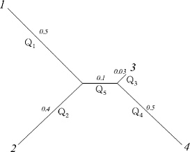
Figure 3: A non-homogeneous tree used for simulations. The numbers labelling each edge correspond to branch lengths (i.e. expected percent change between the two taxa on the edge). (1) In comparing our method with neighbor-joining, the parameters $\alpha_{i},\beta_{i},\gamma_{i}$ in the Kimura 3-parameter rate matrices $Q_{i}$ were chosen as: $\gamma_{1}=1,\alpha_{1}=4,\beta_{1}=1$, $\gamma_{2}=5,\alpha_{2}=14,\beta_{2}=3$ ,$\gamma_{3}=4,\alpha_{3}=15,\beta_{3}=3$, $\gamma_{4}=2,\alpha_{4}=6,\beta_{4}=2$, $\gamma_{5}=2,\alpha_{5}=3,\beta_{5}=1$. (2) In comparing our method with maximum likelihood algorithm based on the Kimura 2-parameter model, we chose $\gamma=\beta=1$ in all rate matrices whereas parameter $\alpha$ was set as follows: in $Q_{1}$, $\alpha=4$, in $Q_{2}$, $Q_{4}$ and $Q_{5}$, $\alpha=3+\varepsilon^{2}$, in $Q_{3}$, $\alpha=3+\varepsilon$. When $\varepsilon=1$ the tree is homogeneous and we studied the efficiency of three methods as $\varepsilon$ increases up to 9.

2. Comparison with maximum likelihood

We compared the invariants method with two versions of maximum-likelihood: the usual maximum likelihood for Kimura 2-parameter [Kim80] and non-homogeneous maximum likelihood method developed in the package PAML [Yan97] for Kimura 2-parameter model (namely, the option nhomo). This last method allows different transition/transversion ratio in different tree branches. To perform this comparison we simulated data according to the tree in figure 3(2) evolving under the Kimura 2-parameter model. When $\varepsilon=1$ the tree is homogeneous and we studied the efficiency of the three methods as $\varepsilon$ increases up to 9.

Figure 4: The effect of rate heterogeneity among lineages on method performance. The simulated nucleotide sequences have length 1000 and evolve under the non-homogeneous Kimura 2-parameter model as described in figure 3 (homogeneous for $\varepsilon=1$). The trees were reconstructed with our method (invariants), with PAML under a non-homogeneous method (PAML non-homogeneous) and the usual PAML maximum likelihood homogeneous (PAML homogeneous). For each $\varepsilon$ 100 sets of data were generated.

Figure 4 summarizes the results relative to the comparison between our method, the non-homogeneous method in PAML for Kimura 2-parameter model (option nhomo=2 in the baseml control file) and the maximum likelihood homogeneous in PAML for Kimura 2-parameter (option nhomo=0). It shows the percentage of correctly reconstructed trees for each value of parameter $\varepsilon$. As expected, the homogeneous maximum-likelihood algorithm becomes less efficient as $\varepsilon$ increases. The use of a method assuming homogeneity on data produced in accord with a non-homogeneous model is, of course, not recommended as such model misspecification is known to lead to unreliable results. Already for $\varepsilon=5$, the invariants method overtakes the homogeneous maximum likelihood algorithm. As it is deduced from figure 4, our method performs worse than the non-homogeneous algorithm in PAML. However, it is worth noticing that in this test we generated data according to Kimura 2-parameter model and the invariants method presented here was developed under Kimura 3-parameter model. Similar results are obtained when the data evolve under Kimura 3-parameter model (see figure II in the Supplementary Material).

Methods

The phylogenetic reconstruction method used in this paper is based on phylogenetic invariants and was first introduced by the first author and L.D. Garcia and S. Sullivant in [CGS05].

The taxa are given by an alignment of $n$ DNA sequences of length $N$. A Markov process along an unrooted binary tree of $n$ species is assumed and we consider that all sites are independently and identically distributed (i.i.d. hypotheses). The parameters of the model we are considering are the entries of the substitution matrices of a Kimura 3-parameter model [Kim81]. (we should rather speak of an algebraic Kimura 3-parameter model, according to the book [PS05, chapters 1 and 4]). Note that in the usual Kimura 3-parameter model, a rate matrix $Q$ is fixed and common to the whole tree and the substitution matrix is the exponential $e^{Qt_{i}}$ (for some parameter $t_{i}$ representing time). However, in our method we do not make use of rate matrices $Q$ —we only use the substitution matrices— so, as we will see later, the rate matrices might vary among the edges. It is worth pointing out that, as we consider a Kimura 3-parameter model along all branches, the uniform distribution of base composition holds for the whole tree (stationarity hypothesis).

Phylogenetic invariants

Sturmfels and Sullivant [SS05] gave an explicit description of the generators of the set of polynomial phylogenetic invariants $I(T)$ for an arbitrary tree evolving under a group-based model. For the Kimura 3-parameter model on an unrooted 4-taxa tree the ideal of phylogenetic invariants has 8002 minimal generators (see the webpage [GP05], [CGS05] and the discussion in [SS05], section 7 to see why a smaller subset of invariants does not suffice). According to the results in [SS05], we produced this generating set for an unrooted tree with 4 leaves under the Kimura 3-parameter model. This requires doing a Fourier transform (or Hadamard conjugation) on the vector of probabilities $(p_{A\dots A},\dots,p_{T\dots T})$ and the phylogenetic invariants are then described as binomials in the Fourier coordinates.

Algorithm

Our tree reconstruction algorithm performs the following tasks. Given 4 aligned DNA sequences $s_{1}$, $s_{2}$, $s_{3}$, $s_{4}$, it first computes the observed relative frequencies of each pattern for the topology $((s_{1},s_{2}),s_{3},s_{4})$ on an unrooted quartet tree. Then it transforms these relative frequencies to Fourier coordinates. From this, we compute the Fourier coordinates in the other two possible topologies for unrooted trees with 4 species. We then evaluate all phylogenetic invariants for the Kimura 3-parameter model in the Fourier coordinates of each tree topology. We call $s_{f}^{T}$ the absolute value of this evaluation for the polynomial $f$ and tree topology $T$. From these values $\{s_{f}^{T}\}_{{}_{f}}$, we produce a score for each tree topology $T$, namely $s(T)=\sum_{f}|s_{f}^{T}|$. The algorithm then chooses the topology that corresponds to the minimum score. The code was written in PERL and is available upon request. For an alignment of 4 sequences of 1000 nucleotides it takes 0.35s on a single 3.0-Ghz processor.

Software used

The simulations of this study were obtained using the program Seq-Gen v1.3.2 [RG97]. We used the algorithms implemented in the package APE [PSC⁺06] v1.8-3 of R [R D05] v2.1.1 to compute Kimura 3-parameter distance [Kim81] and perform neighbor-joining algorithm [SN87]. The package PAML [Yan97] was used for phylogenetic inference involving maximum likelihood methods.

Discussion

The simulation studies performed in this paper present a very competitive phylogenetic reconstruction method based on invariants. If one compares our results on the tree space and those of Huelsenbeck [Hue95] one sees that the method presented here is highly efficient. Note that this might be a biased comparison as in both papers homogeneous models are used for sequence generation and, while he uses homogeneous methods for inference, our invariant method allows non-homogeneous models —remember that one generally obtains the best results using the most restricted model that fits the data. There are some limitations of the tree space study performed here, though. For example, this tree space does not consider trees where the inner edge is extremely small or extremely large with respect to the peripheral branches. As Huelsenbeck points out, the usefulness of considering this parameter space can be questioned, but he also gives strong arguments that convinced us to work in this parameter space. Moreover, considering the same parameter space as Huelsenbeck allows one to compare our results to the other methods studied by him.

We would like to comment on the algorithm presented here and, more generally, on all methods based on invariants. First of all we need to emphasize that the computation of the phylogenetic invariants of a given model just need to be computed once, so their computation need not contribute to the running-time of an algorithm using them. Secondly, increasing the size of the sequences does not drop the computational efficiency of the algorithm. Indeed, the sequences length only accounts for computing the relative frequencies of the observed patterns (which is something that most algorithms based on evolutionary models must do), but it does not participate in any other part of the algorithm.

A small comment on the election of the 1-norm: we performed simulation studies not presented here to prove that the algorithm performs clearly better with the 1-norm than with the maximum norm, and slightly better than with the euclidean norm . Another consideration that might be important for the computational efficiency of the method is that, in Fourier coordinates, the polynomials considered here are binomials and hence they are easy to evaluate at a given point (so there is no need to worry computationally about the evaluation of the polynomials). Moreover, as it is proved in [SS05], these binomials have degree 4 at most so, again, the computational cost is low. Choosing another generating set of invariants or a different weightening of the polynomials will lead to other results, so this is an issue that should certainly be studied in the future.

We implemented and tested the algorithm presented here only on 4-taxon trees. This seems a limitation of the method but as the reader may have noticed, the method is universal and could be used to infer the topology of trees with arbitrary number of taxa. However, the computational demands of deducing large phylogenies led us not to develop this algorithm for larger trees. Instead, we suggest that invariants might be a good starting point for quartet methods of phylogenetic inference. In this direction, it is also worth thinking about new tree reconstruction algorithms for arbitrary taxa based on invariants (this is something the authors will surely work on in the future).

In this paper we focused on the Kimura 3-parameter evolutionary model. However, a full generating set of invariants is known for any group-based model ([SS05]), a large set of invariants is known for the general Markov model [AR03], [AR04a] and for a strand symmetric model [CS05], and some invariants are already known for certain rate-class models [AR06]. Therefore, the method presented here can be extrapolated to these evolutionary models and in the future further models can be considered. In particular, invariants might also perform well for models allowing site-to-site variation.

As we pointed out in the introduction, invariants based methods focus on recovering the tree topology and not estimating the parameters. Nevertheless, as Allman and Rhodes say ([AR03], [AR04b]), it is fair to think that phylogenetic invariants may also be useful for parameter recovery.

As we have already mentioned, one of the advantages of the method presented here versus other methods of phylogenetic reconstruction based on evolutionary models is that the model considered here is non-homogeneous in the sense that the rate matrix is allowed to vary along the different branches of the tree. However, as we are assuming a Kimura model, the base distribution is the same at all nodes of the tree and so the model is stationary (note that invariants methods based on other evolutionary models would not require stationarity of base distribution). For an unrooted tree with $n$ taxa, our algebraic Kimura model has $3(2n-3)$ free parameters, and it is a special case of the general Markov model which involves $12(2n-3)+3$ parameters. If one considered a Kimura 3-parameter model (not the algebraic model considered here) allowing different rate matrices along the tree one would have $3(2n-3)+2n-4$ (the extra parameters correspond to time parameters). Other non-homogeneous models have been considered in the literature, see for example [GG98] and [YR95]. The emphasis in these two papers is put on the non-stationarity hypothesis, and the maximum likelihood approach taken in most non-homogeneous methods makes them computationally unfeasible.

Supplementary material

Supplementary material includes figures I, II, III and IV.

Acknowledgments: The authors would like to thank B. Sturmfels, L. Pachter and N. Eriksson for useful comments on a draft version of the paper. We would also like to thank the reviewers for useful comments that improved the paper. Both authors were partially supported by Ministerio de Educación y Ciencia (Ramón y Cajal and Juan de la Cierva programs, respectively), and BFM2003-06001. The second author was also supported by MTM2005-01518.

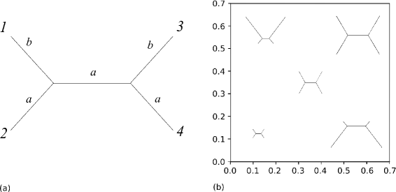
Figure 5: (a) Unrooted 4-taxa tree. The branches labelled with the same letter (either $a$ or $b$) have the same branch length. The taxa are named with arabic numbers, $1$ to $4$. (b) The parameter space for the unrooted four-taxon tree. Parameter $a$ is plotted in the abscissa, while parameter $b$ in the ordinate. The lengths of the branches $a$ and $b$ are varied from $0.01$ to $0.75$ in increments of $2\%$.

Figure 6: The effect of rate heterogeneity among lineages on method performance. The simulated nucleotide sequences have length 1000 and evolve under the non-homogeneous Kimura 3-parameter model for the parameters $\gamma=1,\beta=2$ in all rate matrices while parameter $\alpha$ was set as follows: in $Q_{1}$, $\alpha=4$, in $Q_{2}$, $Q_{4}$ and $Q_{5}$, $\alpha=3+\varepsilon^{2}$, in $Q_{3}$, $\alpha=3+\varepsilon$ (see figure 3). The trees were reconstructed with our method (invariants), and with the usual PAML maximum likelihood homogeneous (PAML homogeneous). For each value of $\varepsilon$, 100 sets of data were generated.

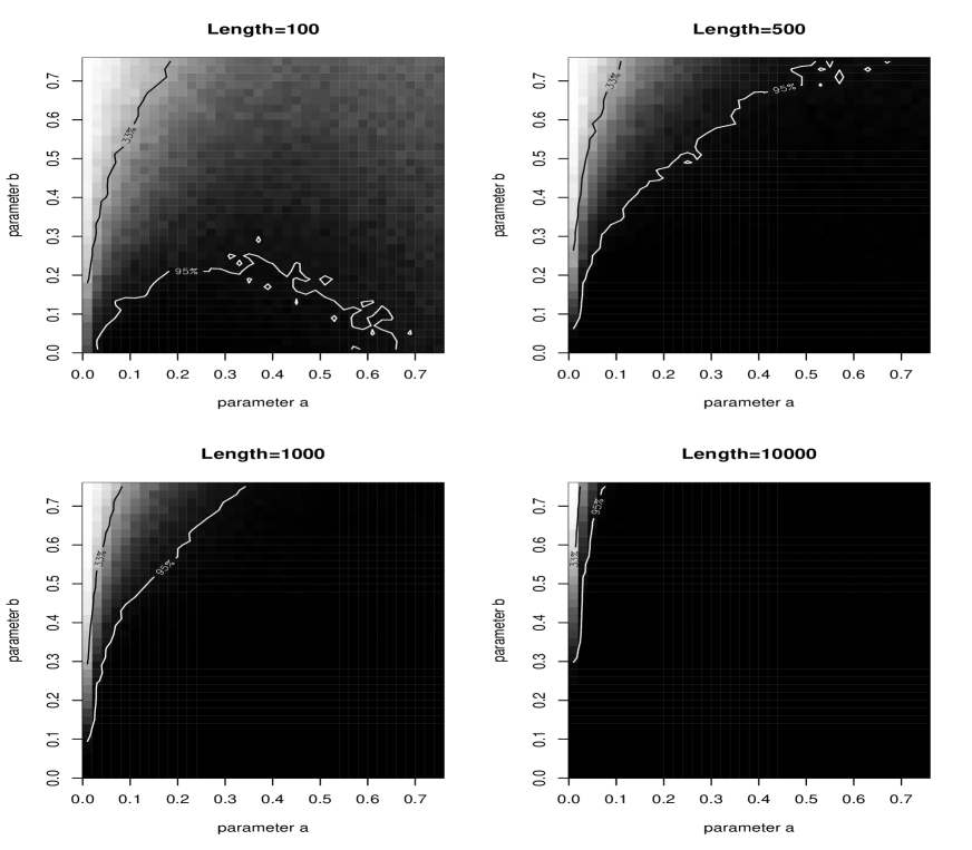
Figure 8: The four graphics above show the results obtained in the four-taxon space when the sequences are generated under the homogeneous Kimura 3-parameter model of substitution using a rate matrix with parameters $\gamma=0.12,\alpha=0.73,\beta=0.13$ (hence a 2.93:1 transition:transversion bias). This rate matrix corresponds to the maximum likelihood estimate from an alignment of homologous sequences of eight vertebrates under a Kimura 3-parameter model.

References

- [AR03] ES Allman and JA Rhodes. Phylogenetic invariants for the general Markov model of sequence mutation. Mathematical Biosciences, 186(2):113–144, 2003.
- [AR04a] ES Allman and JA Rhodes. Phylogenetic ideals and varieties for the general Markov model. to appear in Advances in Applied Mathematics, 2004.
- [AR04b] ES Allman and JA Rhodes. Quartets and parameter recovery for the general Markov model of sequence mutation. AMRX Applied Mathematics Research Express, 2004(4):107–131, 2004.
- [AR06] ES Allman and JA Rhodes. The identifiability of tree topology for phylogenetic models, including covarion and mixture models. J. Comput. Biol., 13:1101–1113, 2006.
- [CF87] J Cavender and J Felsenstein. Invariants of phylogenies in a simple case with discrete states. J. Classification, 4:57–71, 1987.
- [CGS05] M Casanellas, LD Garcia, and S Sullivant. Catalog of small trees. In L. Pachter and B. Sturmfels, editors, Algebraic Statistics for Computational Biology, chapter 15. Cambridge University Press, 2005.
- [CS05] M Casanellas and S Sullivant. The strand symmetric model. In L. Pachter and B. Sturmfels, editors, Algebraic Statistics for Computational Biology, chapter 16. Cambridge University Press, 2005.
- [Eri05] N Eriksson. Tree construction using singular value decomposition. In L. Pachter and B. Sturmfels, editors, Algebraic Statistics for Computational Biology, chapter 19, pages 347–358. Cambridge University Press, 2005.
- [ES93] S Evans and T Speed. Invariants of some probability models used in phylogenetic inference. The Annals of Statistics, 21:355–377, 1993.
- [Fel81] J Felsenstein. Evolutionary trees from DNA sequences: a maximum likelihood approach. J Mol Evol., 17:368–376, 1981.
- [Fel03] J Felsenstein. Inferring Phylogenies. Sinauer Associates, Inc., 2003.
- [FS95] V Ferretti and D Sankoff. Phylogenetic invariants for more general evolutionary models. J. Theor. Biol., 147-162, 1995.
- [GG98] N Galtier and M Gouy. Inferring pattern and process: maximum likelihood implementation of a non-homogeneous model of DNA sequence evolution for phylogenetic analysis. Mol. Biol. Evol., 154(4):871–879, 1998.
- [GP05] L D Garcia and J Porter. Small phylogenetic trees webpage. http://bio.math.berkeley.edu/ascb/chapter15/, 2005.
- [HL00] TR Hagedorn and LF Landweber. Phylogenetic invariants and geometry. J. Theor. Biol., 205:365–376, 2000.
- [Hue95] JP Huelsenbeck. Performance of phylogentic methods in simulation. Syst. Biol., 44:17–48, 1995.
- [JN90] L Jin and M Nei. Limitations of the evolutionary parsimony method of phylogenetic analysis. Mol. Biol. Evol., 7:82–102, 1990.
- [Kim80] M Kimura. A simple method for estimating evolutionary rates of base substitution through comparative studies of nucleotide sequences. J. Mol. Evol., 16:111–120, 1980.
- [Kim81] M Kimura. Estimation of evolutionary sequences between homologous nucleotide sequences. Proc. Nat. Acad. Sci. , USA, 78:454–458, 1981.
- [KKPP06] Y Rock Kim, O Kwon, S Paeng, and C Park. Phylogenetic tree constructing algorithms fit for grid computing with SVD. Preprint July, 2006.
- [Lak87] J.A. Lake. A rate-independent technique for analysis of nucleaic acid sequences: evolutionary parsimony. Mol. Biol. Evol., 4:167–191, 1987.
- [PS05] L Pachter and B Sturmfels, editors. Algebraic Statistics for Computational Biology. Cambridge University Press, November 2005. ISBN 0-521-85700-7.
- [PSC+06] Emmanuel Paradis, Korbinian Strimmer, Julien Claude, Gangolf Jobb, Rainer Opgen-Rhein, Julien Dutheil, Yvonnick Noel, Ben Bolker, and Jim Lemon. ape: Analyses of Phylogenetics and Evolution, 2006. R package version 1.8-3.
- [R D05] R Development Core Team. R: A language and environment for statistical computing. R Foundation for Statistical Computing, Vienna, Austria, 2005. ISBN 3-900051-07-0.
- [RG97] A Rambaut and NC Grassly. Seq-Gen: An application for the Monte Carlo simulation of DNA sequence evolution along phylogenetic trees. Comput. Appl. Biosci., 13:235–238, 1997.
- [SB99] D Sankoff and M Blanchette. Phylogenetic invariants for genome rearrangements. J. Comput. Biol., 6:431–445, 1999.
- [SN87] N Saitou and M Nei. The neighbor joining method: a new method for reconstructing phylogenetic trees. Mol. Biol. Evol., 4(4):406–425, 1987.
- [SS05] B Sturmfels and S Sullivant. Toric ideals of phylogenetic invariants. J. Comput. Biol., 12:204–228, 2005.
- [SSEW93] MA Steel, LA Székely, PL Erdős, and P Waddell. A complete family of phylogenetic invariants for any number of taxa under Kimura’s 3st model. New Zealand Journal of Botany, 31:289–296, 1993.
- [Yan97] Z Yang. PAML: A program package for phylogenetic analysis by maximum likelihood. CABIOS, 15:555–556, 1997.
- [YR95] Z Yang and D Roberts. On the use of nucleic acid sequences to infer early branchings in the tree of life. Mol. Biol. Evol., 12:451–458, 1995.
- [YY99] Z Yang and A D Yoder. Estimation of the transition/transversion rate bias and species sampling. J. Mol. Evol., 48:274–283, 1999.