Bayesian analysis of biological networks: clusters, motifs, cross-species correlations

The complexity of an organism is only weakly linked with its number of genes. Homo sapiens has about 25000 genes and the roundworm C. elegans about 19000 [1, 2], despite the different level of complexity. Not only the gene numbers are similar, the genes themselves are frequently shared across species. Even distantly related organisms have a high fraction of genes which stem from their common ancestor (orthologs): more than $90\%$ of genes are shared between human and mouse and at least $30\%$ of genes of the yeast S. cerevisiae have orthologs in human [3].

This result is an important outcome of the recent genome sequencing projects. It has put the spotlight on the interactions between genes: changes in the complex networks of gene regulation, or in the interactions between proteins, may be a major cause of phenotypic variation, more so than changes in the genes themselves [4]. The molecular basis of these interactions includes specific binding sites on regulatory DNA and binding domains in proteins. Binding sites can change quickly generating new interactions or deleting old ones [5, 6, 7, 8].

The resulting interest in biological interactions has been matched by the development of novel experimental techniques to measure protein–DNA interactions and protein–protein interactions. In particular, high-throughput methods have been developed, facilitating measurements on a genome-wide scale rather than for individual genes. Some of the ingenious methods for experimentally determining biological interactions will be briefly reviewed in the next section.

This experimental development is akin to the transition from sequencing small parts of the DNA of an organism to the determination of full genomes. The growth of sequencing capabilities has been driving the development of computational methods for sequence analysis for the past three decades. Virtually all methods for sequence analysis rely on statistics as a tool to infer function. Examples are the detection of genes, or of regulatory modules, or the identification of correlations between evolutionarily related sequences [9].

The corresponding development of computational network biology is still in its infancy. It will require new tools to address specific issues of biological networks. These are characterized by a peculiar interplay of stochasticity and function, and in many ways epitomize our current lack of understanding of biological systems. With this caveat, the point of view we take in this article is that statistics will again play a decisive role in our understanding of network biology, and we point out some currently available links between network statistics and function. The merit of a statistical approach may not seem obvious from an engineering perspective, where networks are seen as deterministic processing machines producing a well-defined input–output relation. Indeed, biological networks sometimes work in a surprisingly deterministic way: for example, a network of a few dozen major genes generates a well-defined spatiotemporal development pattern in the eukaryotic embryo. However, the underlying network structures are fundamentally stochastic, since they arise from the manifold tinkering and feedback processes of biological evolution. Explaining deterministic function from a stochastic evolution requires a statistical, dynamical theory.

One important aspect of this challenge is to predict different functional units in networks. Different functions are reflected in a different evolutionary dynamics, and hence in different statistical characteristics of network parts. In this sense, the global statistics of a biological network, e.g., its connectivity distribution, provides a background, and local deviations from this background signal functional units. In the computational analysis of biological networks, we thus typically have to discriminate between different statistical models governing different parts of the dataset. The nature of these models depends on the biological question asked. We illustrate this rationale here with three examples: identification of functional parts as highly connected network clusters, finding network motifs, which occur in a similar form at different places in the network, and the analysis of cross-species network correlations, which reflect evolutionary dynamics between species.

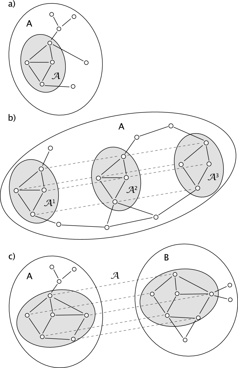
Figure 1: Deviation from a uniform global statistics in biological networks. a) A network cluster is distinguished by an enhanced number of intra-cluster interactions. b) A network motif is a set of subgraphs with correlated interactions. In a limiting case, all subgraphs have the same topology. c) Cross-species correlations characterize evolutionarily conserved parts of networks.

1. Measuring biological networks

A wide range of experimental methods has been developed to measure interactions between proteins, interactions between proteins and regulatory DNA, and expression levels of genes. Only a brief review is possible here.

In the yeast-two-hybrid (Y2H) method, the pairwise interaction between two proteins is tested by creating two fusion proteins [10]. One protein is constructed with a DNA-binding domain attached to its end, and its potential binding partner is fused to an activation domain. If the two proteins interact, the binding will form a transcriptional activator (generally consisting of a DNA-binding domain and an activation domain). The presence of an intact activator leads to the transcription of an easily detectable reporter gene. (The reporter gene may for instance produce a fluorescent protein.) In principle, the amount of the reporter gene produced can serve as a measure of the affinity between the two proteins. The Y2H-method has been used to measure the protein interaction networks of yeast [10], C. elegans [11], D. melanogaster [12], and human [13]. The Y2H-datasets are known to contain a large number of false positive and false negative results. False negatives arise when the fusion proteins fail to localize in the yeast nucleus, or fail to fold properly once the new domains are attached. False positives may be linked to high expression levels of the hybrid in yeast, which are never reached in vivo.

Alternative approaches include pull-down assays, where one protein type is immobilized on a gel, and ‘pulls down’ binding partners from a solution. Binding partners may then be identified by various tags. Mass spectrometry is also used to identify the interacting protein pairs identified by such an affinity analysis [14]. While more accurate than the Y2H-method, these approaches have not yet been scaled up to provide high throughputs.

Binding of proteins, specifically transcription factors, to regulatory DNA has long been investigated by electrophoresis, where the motility of a DNA-fragment is altered by a protein bound to it. Chromatin immunoprecipitation (ChIP) is an alternative procedure, which uses specific antibodies to isolate a protein and then amplifies DNA that may have been isolated together (co-precipitated) with the protein. By running many such experiments in parallel on a microarray, this method can be scaled up to high throughputs (ChIP-on-chip, [15]).

Gene expression levels can be measured on DNA-microarrays, densely packed samples of known nucleotides, each a few tens of base-pairs long. Currently more than $10^{6}$ such samples, or probes, can be placed on a single microarray. The array is then washed with a fluorescently labeled sample. Binding of DNA in the sample to complementary DNA on the probe can be detected under a microscope from the resulting fluorescence pattern. Genome-wide expression levels can thus be measured on a single array. Many other applications of microarrays are being developed — for instance microarrays to measures interactions between transcription factors and regulatory DNA. DNA-microarrays are also making major inroads as diagnostic tools, from characterizing the microbial communities in dentistry [16] to the early detection of cancer [17].

2. Random networks in biology

Randomly generated networks are very useful to analyze simple characteristics of biological networks. For instance, typical distances on a randomly generated network generally scale logarithmically with the number of network nodes. Finding such short distances also in biological network data is therefore not a surprising result and does not require a biological explanation. Another frequent observation in biological networks is a distribution of node connectivities with a broad tail, which is shared by specific ensembles of random networks. This has motivated a number of statistical models explaining the connectivity distribution in terms of the underlying evolutionary dynamics [18, 19, 20]. Thus, ensembles of random networks can be tuned to fit certain characteristics of biological network data. Does that mean the actual network is random? This is clearly not the case: other observables may differ from what is expected in the random network ensemble, and we will see that these deviations from the “null model” are particularly interesting as signals of biological function. Hence, random network ensembles play an important role in quantifying the most unbiased background statistics of a “functionless” network. Their choice is a subtle issue: it has to be motivated by what we consider as not important for the biological function in question. Let us now turn to a few such models.

A network is specified by its adjacency matrix ${\bf a}=(a_{ii^{\prime}})$. For binary networks $a_{ii^{\prime}}=1$ if there is a link between nodes $i$ and $i^{\prime}$, and $a_{ii^{\prime}}=0$ if there is no link. Networks with undirected links are represented by a symmetric adjacency matrix. The in and out connectivities of a node, $k^{+}_{i}=\sum_{i^{\prime}}a_{i^{\prime}i}$ and $k^{-}_{i}=\sum_{i^{\prime}}a_{ii^{\prime}}$, are defined as the number of in- and outgoing links, respectively. The total number of directed links is given by $K=\sum_{i,i^{\prime}}a_{ii^{\prime}}$.

To focus on a specific part of the network we define an ordered subset ${\cal A}$ of $n$ nodes $\{r_{1},\dots r_{n}\}$ (see Fig. 1a). The subset ${\cal A}$ induces a pattern $\hat{\bf a}({\cal A})$ on the network, represented by the restricted adjacency matrix containing only links internal to node subset ${\cal A}$. $\hat{\bf a}$ is thus an $n\times n$ matrix with entries $\hat{a}_{ij}=a_{r_{i}r_{j}}$ ($i,j=1,\dots,n$). Together, subset of nodes ${\cal A}$ and its pattern $\hat{\bf a}({\cal A})$ form a subgraph.

The simplest ensemble of random networks is generated by connecting all pairs of nodes independently with the same probability $w$. Given a subset of nodes ${\cal A}$, the probability of generating pattern $\hat{\bf a}$ is then given by $P_{0}({\bf a})=\prod_{i,i^{\prime}\in{\cal A}}^{n}(1-w)^{1-a_{ii^{\prime}}}w^{a_{ii^{\prime}}}$ (for undirected networks the sum is restricted to $i\leq i^{\prime}$). This well-known ensemble, named after the pioneers of graph theory P. Erdős and A. Rényi, leads to a Poissonian distribution of connectivities. The only free parameter of the Erdős–Rényi (ER) model, the link probability $w$ between a given pair of nodes, can be tuned so that typical graphs taken from the ER-ensemble have the same number of links as the empirical data. If the subset of nodes ${\cal A}$ contains all $n=N$ nodes of the network, $w=K/N^{2}$. Considering connected subgraphs with $n<N$, $w$ will in general be higher than $K/N^{2}$. Then the value of $w$ can be determined by generating all connected subgraphs of size $n$ from the empirical dataset and choosing $w$ such that the average number of links in the ER model equals the average number of links in connected subgraphs in the data.

However, in biological networks the connectivity distribution often differs markedly from that of the Erdős–Rényi-model. If we have reasons to assume that a biological function is not tightly linked to connectivity at the level of individual nodes, we should include the connectivity distribution in our null model. Indeed, we can easily construct a random ensemble matching the connectivity distribution of the dataset. In this ensemble, the probability $w_{ii^{\prime}}$ of finding a link between a pair of nodes $i$, $i^{\prime}$ depends on the connectivities of the nodes. Assuming links between different node pairs to be uncorrelated, a given subset of nodes ${\cal A}$ has a pattern $\hat{\bf a}$ with probability

$$P_{0}(\hat{\bf a})=\prod_{i,i^{\prime}\in{\cal A}}^{n}(1-w_{ii^{\prime}})^{1-a_{ii^{\prime}}}w_{ii^{\prime}}^{a_{ii^{\prime}}}.$$ (1)

For $n=N$, when ${\cal A}$ includes the entire network, the probability of finding a directed link between nodes $i$ and $i^{\prime}$ is approximately $w_{ii^{\prime}}=k^{-}_{r_{i}}k^{+}_{r_{i^{\prime}}}/K$, that of an undirected link $w_{ii^{\prime}}=k_{r_{i}}k_{r_{i^{\prime}}}/K$ [21]. If we furthermore impose the constraint that the null model describe the statistics of a connected dataset, the probabilities in (1) are increased by a factor that can be determined from the data as described above. The null model constructed in this way is maximally unbiased with respect to all patterns in the dataset beyond its connectivity distribution.

3. Network clusters

A first trace of functionality in biological networks are strong inhomogeneities in their link statistics, which are not captured by the null model. Examples are protein aggregates of several proteins held together by mutual interactions, which show up as highly connected clusters in protein interaction networks, and sets co-regulated genes (for instance by an oncogene [22]), leading to clusters in co-expression networks. How can we identify these clusters statistically?

Clusters are subgraphs with a significantly increased number of internal links compared to the background of the network, see Figure 1a). The feature distinguishing clusters is the number of internal links,

$$L(\hat{\bf a})=\sum_{i,i^{\prime}\in{\cal A}}^{n}\hat{a}_{ii^{\prime}}\ .$$ (2)

The statistics of clusters is then described by an ensemble

$$Q_{\sigma}(\hat{\bf a})=Z_{\sigma}^{-1}\exp[\sigma L(\hat{\bf a})]\,P_{0}(\hat{\bf a})$$ (3)

of the same form as (1), but with a bias towards a high number of internal links. The average number of internal links is determined by the value of the link reward $\sigma$. We have introduced the normalization factor $Z_{\sigma}=\prod_{ii^{\prime}}^{n}\sum_{\hat{a}_{ii^{\prime}}=0,1}\exp[\sigma L(\hat{\bf a})]\,P_{0}(\hat{\bf a})$, which ensures that $Q_{\sigma}(\hat{\bf a})$ summed over all patterns $\hat{\bf a}$ gives unity.

Is a given pattern $\hat{\bf a}$ more likely part of a cluster as described by the model (3), or is it more likely part of the background described by the null model (1)? To address this question, we define the so-called log-likelihood score

$$S({\cal A},\sigma)=\log\left(\frac{Q_{\sigma}(\hat{\bf a})}{P_{0}(\hat{\bf a})}\right)=\sigma L(\hat{\bf a}({\cal A}))-\log Z_{\sigma}\ .$$ (4)

A positive score results if it is more likely for the pattern $\hat{\bf a}({\cal A})$ to arise in the model describing clusters than in the alternative null model. High scores indicate strong deviations from the null model. Of course this an attractive property for the algorithmic search for deviations from the null model. As shown in the appendix, the form of the score (4) is related in a simple way to the probability that pattern $\hat{\bf a}$ comes from the model describing clusters.

Patterns with a high score (4) are bona fide clusters. The first term of the score weighs the total number of links. As expected, a pattern with many internal links yields a high score. The second term acts as a threshold and assigns a negative score to a pattern with a too small number of internal links. This term takes into account the connectivities of the nodes: highly connected nodes have more internal links already in the null model. Node subsets with highly connected nodes tend to give lower scores. The score (4) thus goes beyond simple measures of clustering, such as the number of internal links, and provides a statistical basis for cluster detection.

a)

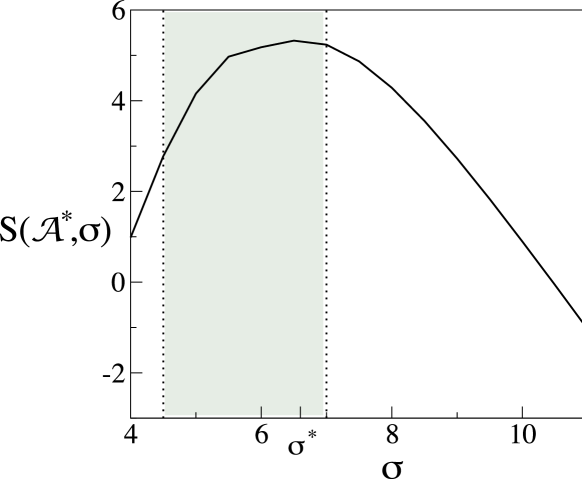
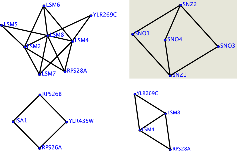
b)

Figure 2: Scoring clusters in protein interaction networks. a) The score $S$ of the maximum-score node subset ${\cal A}^{\star}(\sigma)$ is shown as a function of the scoring parameter $\sigma$. The dotted lines indicate the values of $\sigma$ where the maximum-score node subset changes. The maximum of the score with respect to $\sigma$ indicates the optimal scoring parameter $\sigma^{\star}=6.6$. The grey region $4.25<\sigma<7$ indicates the values where ${\cal A}^{\star}(\sigma)={\cal A}^{\star}(\sigma^{\star})$. b) The maximum-score subgraphs for $\sigma<4.25$, $4.25<\sigma<7$, $7<\sigma<11$,$\sigma>11$ (left to right). The subgraph resulting from the optimal scoring parameter is highlighted in grey. The maximum-score subgraphs for $7<\sigma<11$ and for $\sigma>11$ are distinguished by the connectivities of their nodes with the latter having a higher average connectivity. This accounts for the former having a higher score for $7<\sigma<11$ despite the smaller number of internal links.

Given the scoring parameter $\sigma$, the maximum-score node subset ${\cal A}^{\star}(\sigma)$ is defined by

$${\cal A}^{\star}(\sigma)=\mbox{argmax}_{{\cal A}}S({\cal A},\sigma)\ .$$ (5)

At this point, the scoring parameter $\sigma$ is a free parameter, whose value needs to be inferred from the data. This can be done by applying the principle of maximum likelihood: $\sigma$ is determined by the requirement that the model describing clusters (3) optimally describes the statistics of the maximum-score pattern. For a given pattern $\hat{\bf a}$, the optimal fit is defined by the so-called maximum likelihood value $\sigma^{\star}=\mbox{argmax}_{\sigma}Q_{\sigma}(\hat{\bf a}({\cal A}))$, which maximizes the likelihood of generating pattern $\hat{\bf a}({\cal A})$ under the model (3). Since $\log(x)$ is a monotonously increasing function, the maximum likelihood value $\sigma^{\star}$ coincides with the maximum of the log-likelihood score (4) over $\sigma$. The maximum-score node subset at the optimal scoring parameter is then determined by the joint maximum of the score over ${\cal A}$ and $\sigma$

$$S({\cal A}^{\star},\sigma^{\star})=\max_{\sigma}S({\cal A}^{\star}(\sigma),\sigma)=\max_{{\cal A},\sigma}S({\cal A},\sigma)\ .$$ (6)

One can easily show that the maximum-likelihood value of $\sigma$ sets the expected number of links in the ensemble $Q_{\sigma^{\star}}$ equal to the actual number of links in pattern $\hat{\bf a}^{\star}$: setting the derivative of (4) with respect to $\sigma$ equal to zero gives

$$\langle L(\hat{\bf a})\rangle_{Q_{\sigma^{\star}}}=L(\hat{\bf a}^{\star})\ .$$ (7)

Clusters in protein interaction networks. We use the scoring function (4) to identify clusters in the protein interaction network of yeast, namely the high-throughput dataset of Uetz et al. [10]. At a given value of the scoring parameter $\sigma$, the maximum-score node subset ${\cal A}^{\star}(\sigma)$ is identified using a simple Monte-Carlo algorithm. At different values of $\sigma$, different node subsets ${\cal A}^{\star}(\sigma)$ yield the highest score (compared to all other node subsets). The resulting subgraphs are shown in Fig. 2a). At low values of $\sigma$, subgraphs with many nodes, but comparatively few internal interactions per node yield the highest score. At high values of $\sigma$, subgraphs with many internal interactions are favored. However these subgraphs tend to be small. The interplay between subgraph size and internal connectivity leads to a joint score maximum over ${\cal A}$ and $\sigma$ at the optimal scoring parameter $\sigma^{\star}=6.6$, see Fig. 2a).

The maximum-score cluster ${\cal A}^{\star}\equiv{\cal A}^{\star}(\sigma^{\star})$ consists of the proteins SNZ1,SNZ2,SNO1,SNO3, and SNO4, highlighted in grey in Fig. 2 b). The proteins in this cluster have a common function; they are involved in the metabolism of pyridoxine and in the synthesis of thiamin [23, 24]. Furthermore, SNZ1 and SNO1 have been found to be co-regulated and their mRNA levels increase in response to starvation for aminoacids A, Ura, and Trp [25].

4. Network motifs

The topology of a subgraph may be associated with a specific function. A possible example is a feed-forward loop acting as a high-frequency filter in a regulatory network [26]. If such a function is required repeatedly in different parts of the network, there is selection pressure for the creation and maintenance of similar topologies in different parts of a network. Such network motifs [27, 26] are families of subgraphs distinguished from the null model by mutual correlations between subgraphs, see Fig. 1 b).

To quantify these correlations, we need to specify the parts of the network with correlated patterns. We define a graph alignment ${\cal A}$ by a set of several node subsets ${\cal A}^{\alpha}$ ($\alpha=1,\dots,p$), each containing the same number of $n$ nodes, and a specific order of the nodes $\{r_{1}^{\alpha},\dots,r_{n}^{\alpha}\}$ in each node subset. An alignment associates each node in a node subset with exactly one node in each of the other node subsets. The alignment can be visualized by $n$ “strings”, each connecting $p$ nodes as shown in Fig. 1(b).

An alignment specifies a pattern $\hat{\bf a}^{\alpha}\equiv\hat{\bf a}({\cal A}^{\alpha},{\cal A})$ in each node subset. For any two aligned subsets of nodes, ${\cal A}^{\alpha}$ and ${\cal A}^{\beta}$, we can define the pairwise mismatch of their patterns

$$M(\hat{\bf a}^{\alpha},\hat{\bf a}^{\beta})=\sum_{i,i^{\prime}=1}^{n}[\hat{a}_{ii^{\prime}}^{\alpha}(1-\hat{a}_{ii^{\prime}}^{\beta})+(1-\hat{a}_{ii^{\prime}}^{\alpha})\hat{a}_{ii^{\prime}}^{\beta}]\ .$$ (8)

The mismatch is a Hamming distance for aligned patterns. The average mismatch over all pairs of aligned patterns is termed the fuzziness of the alignment.

Frequently network motifs also have an enhanced number of internal links [26, 27], providing the possibility of feedback or other faculties not available to tree-like patterns. An ensemble describing $p$ node subsets with correlated patterns $\hat{\bf a}^{1},\dots,\hat{\bf a}^{p}$ with an enhanced number of links is given by

$$Q_{\mu,\sigma}(\hat{\bf a}^{1},\dots,\hat{\bf a}^{p})=Z_{\mu,\sigma}^{-1}\prod_{\alpha=1}^{p}P_{0}(\hat{\bf a}^{\alpha})$$

$$\times\exp\left[-\frac{\mu}{2p}\sum_{\alpha,\beta=1}^{p}M(\hat{\bf a}^{\alpha},\hat{\bf a}^{\beta})+\sigma\sum_{\alpha=1}^{p}L(\hat{\bf a}^{\alpha})\right]\ .$$

The parameter $\mu\geq 0$ biases the ensemble (4. Network motifs) towards patterns with small mutual mismatches $M(\hat{\bf a}^{\alpha},\hat{\bf a}^{\beta})$.

Given the null model (1) and the model (4. Network motifs) with correlated patterns, we obtain a log-likelihood score for network motifs

$$S({\cal A},\mu,\sigma)$$ (10)

$$= \log\left(\frac{Q_{\mu,\sigma}(\hat{\bf a}^{1},\dots,\hat{\bf a}^{p})}{P_{0}(\hat{\bf a}^{1},\dots,\hat{\bf a}^{p})}\right)$$

$$= -\frac{\mu}{2p}\sum_{\alpha,\beta=1}^{p}M(\hat{\bf a}^{\alpha},\hat{\bf a}^{\beta})+\sigma\sum_{\alpha=1}^{p}L(\hat{\bf a}^{\alpha})$$

$$-\log Z_{\mu,\sigma}\ .$$

High-scoring alignments ${\cal A}$ indicate bona fide network motifs. The first and second term reward alignments with a small mutual mismatch and a high number of internal links, respectively. The term $\log Z_{\sigma,\mu}$ acts as a threshold assigning a negative score to alignments with too high fuzziness or too few internal links.

Again, both the alignment ${\cal A}$ and the scoring parameters $\mu$ and $\sigma$ are a priori undetermined. For given scoring parameters, the maximum-score alignment

$${\cal A}^{\star}(\mu,\sigma)=\mbox{argmax}_{{\cal A}}S({\cal A},\mu,\sigma)$$ (11)

occurs at some finite value of the number of subgraphs $p^{\star}(\mu,\sigma)$.

The scoring parameters $\mu$ and $\sigma$ can again be determined by maximum likelihood, which corresponds to maximizing the score $S({\cal A}^{\star}(\mu,\sigma),\mu,\sigma)$ with respect to the scoring parameters. By differentiating (10) with respect to the scoring parameters one finds that at $\mu=\mu^{\star}$ and $\sigma=\sigma^{\star}$ the model (4. Network motifs) fits the maximum-score network motifs: the expectation values of the internal number of links and the fuzziness equal the corresponding values of the maximum-score alignment.

Network motifs in regulatory networks. We now apply the scoring function (10) to the identification of network motifs in the gene regulatory network of E. coli, taken from [26]. A full account and a score-maximization algorithm are given in [28].

(a)

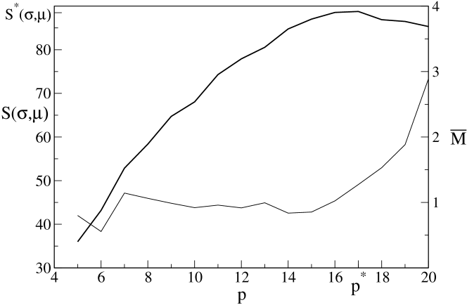
(b)

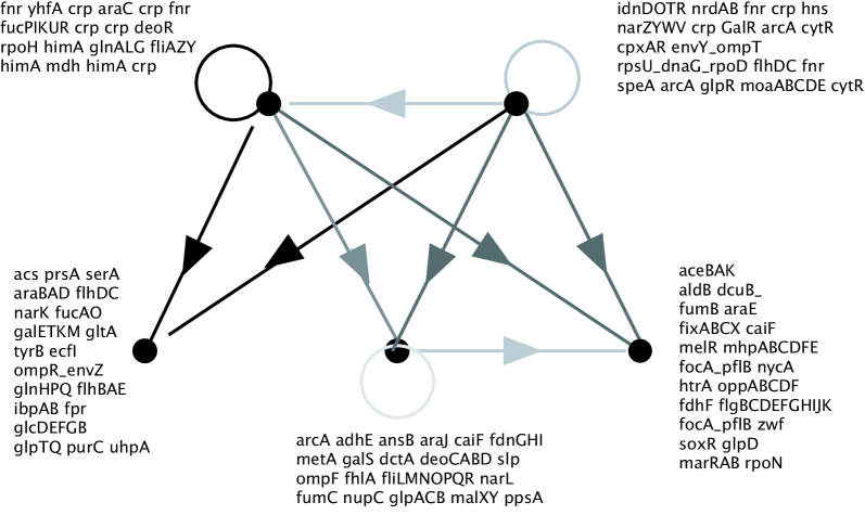
Figure 3: Motifs in the regulatory network of E. coli. (a) Score optimization at fixed scoring parameters $\sigma=3.8$ and $\mu=4.0$ for subgraphs of size $n=5$. The total score $S$ (thick line) and the fuzziness ${\overline{M}}$ (thin line) are shown for the highest-scoring alignment of $p$ subgraphs, plotted as a function of $p$. (b) The consensus motif of the optimal alignment, and the identities of the genes involved. The alignment consists of $18$ subgraphs sharing at most one node. The $5$ grey values correspond to the consensus motif $\overline{a}$ in the range $0.1-0.2$, $0.2-0.4$, $0.4-0.6$, $0.6-0.8$, $0.8-0.9$.

We first investigate the properties of the maximal score alignment at fixed scoring parameters. Fig. 3 (a) shows the score $S$ and the fuzziness ${\overline{M}}$ for the highest-scoring alignment with a prescribed number $p$ of subgraphs, plotted against $p$. The fuzziness increases with $p$, and the score reaches its maximum $S^{\star}(\sigma,\mu)$ at some value $p^{\star}(\sigma,\mu)$. For $p<p^{\star}(\sigma,\mu)$ the score is lower, since the alignment contains fewer subgraphs and for $p>p^{\star}(\sigma,\mu)$ it is lower since the subgraphs have higher mutual mismatches.

The optimal scoring parameters $\mu$ and $\sigma$ are again inferred by maximum likelihood. The resulting optimal alignment ${\cal A}^{\star}\equiv{\cal A}^{\star}(\mu^{\star},\sigma^{\star})$ is shown in Fig. 3 (b) using the so-called consensus motif

$$\overline{\bf a}=\frac{1}{p}\sum_{\alpha=1}^{p}{\hat{\bf a}}^{\alpha}({\cal A}^{\star})\ .$$ (12)

The consensus motif is a probabilistic pattern; the entry $\overline{a}$ denotes the probability that a given binary link is present in the aligned subgraphs. The motif shown in Fig. 3 (b) consists of $2+3$ nodes forming an input and an output layer, with links largely going from the input to the output layer. Most genes in the input layer code for transcription factors or are involved in signaling pathways. The output layer mainly consists of genes coding for enzymes.

5. Cross-species analysis of networks

The motifs discussed above show correlation without sharing a common evolutionary history. Larger functional units may be distinguished by their evolutionary conservation. Thus, we expect parts of the network to maintain their topology and to form a conserved core, while other parts show a more rapid turnover of both nodes and interactions, see Figure 1c). This conservation can be detected as topological correlation across species.

We assume that organisms evolve independently after speciation, leading to divergence in their network links as well as in the overall similarity of the nucleotide sequences, the structure of proteins, and the biochemical role of a metabolite. The relationship between link and node similarity is non-trivial: genes may retain their function and their interactions with other genes despite considerable sequence divergence. On the other hand, the change of a few nucleotides can create or destroy a binding site, implying that genes with high overall sequence similarity may have entirely different interactions. Hence, the cross-species analysis has to take into account information from both links and nodes.

A log-likelihood score assessing the link statistics of node subsets in network $A$ and in network $B$ follows directly from (10). This link score is given by

$$S^{\ell}({\cal A},\mu,\sigma_{A},\sigma_{B})=-\mu M(\hat{\bf a},\hat{\bf b})$$

$$+\sigma\left(L(\hat{\bf a})+L(\hat{\bf b})\right)-\log Z_{\mu,\sigma}\ .$$

To assess the similarity of nodes, we consider a measure $\theta_{ij}$, which describes the similarity of node $i$ in network $A$ and node $j$ in network $B$. The node similarity measure may be a percentage sequence identity, or a distance measure of protein structures. The information on node similarity can be incorporated into the alignment score by contrasting a null model with a model describing a statistics where node similarity is correlated with the alignment. To construct the null model, we assume that node similarities $\theta_{ij}$ for different node pairs $i,j$ are identically and independently distributed and denote their distribution by $p_{0}^{n}(\theta_{ij})$. The model describing cross-species correlations has to take into account that the distribution of node similarities between aligned pairs of nodes follows a different statistics (typically generating higher values of $\theta$), denoted by $q^{n}_{1}(\theta)$. The distribution of pairwise similarity coefficients between one aligned node and nodes other than its alignment partner is denoted by $q^{n}_{2}(\theta)$.

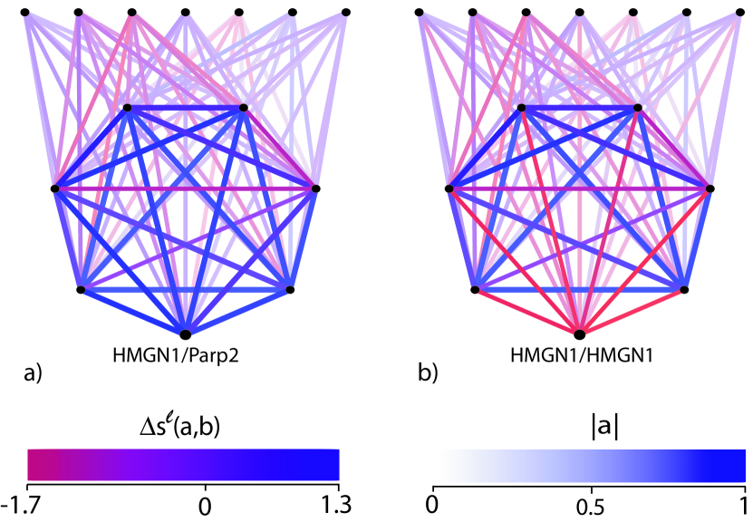
Figure 4: Cross-species network alignment shows conservation of gene clusters. (a) $7$ genes from a cluster of co-expressed genes (circle) together with $7$ random genes outside the cluster (straight line). Each node represents a pair of aligned genes in human and mouse. The intensity of a link encodes the correlation value $a$ in human. The color indicates the evolutionary conservation of a link, with blue hues indicating strong conservation. Th conservation is quantified by the excess link score contribution, $\Delta s^{\ell}$, defined as the link score minus the average link score of links with the same correlation value. (b) The same cluster, but with human-HMGN1 “falsely” aligned to its ortholog mouse-HMGN1, with the red links showing the poor expression overlap of this pair of genes.

Assuming that the statistics of links and nodes similarities are uncorrelated for a given alignment, a simple calculation analogous to (4) yields the log-likelihood score

$$S({\cal A})=S^{\ell}({\cal A})+S^{n}({\cal A})\ ,$$ (14)

with the information from node similarity contributing a node score

$$S^{n}({\cal A})=\sum_{i\in{\cal A}}s^{n}_{1}(\theta_{ii})+\sum_{\scalebox{0.75}{ \parbox{71.13188pt}{$i\in{\cal A},j\neq i$ \\ $j\in{\cal B},i\notin{\cal A}$ } }}s^{n}_{2}(\theta_{ij})$$ (15)

and $s^{n}_{1}(\theta)\equiv\log\left(q^{n}_{1}(\theta)/p_{0}^{n}(\theta)\right)$ and $s^{n}_{2}(\theta)\equiv\log\left(q^{n}_{2}(\theta)/p_{0}^{n}(\theta)\right)$.

The scoring parameters entering (14) need to be determined from the data. Provided there are not too many scoring parameters, this can again be done by maximum likelihood as outlined in the preceding sections. Particular examples are networks with binary links and course-grained measures of sequence similarity. (As an extreme case, node similarity may be considered a binary variable, when nodes either have significant similarity or not. Then the ensembles describing the node statistics are each described by a single variable, see [29] for details.)

Alignment of co-expression networks. We compare co-expression networks of H. sapiens and M. musculus. In co-expression networks, the weighted link $a_{ii^{\prime}}\in[-1,1]$ between a pair of genes $i,j$ is given by the correlation coefficient of their gene expression profiles measured on a microarray chip. Genes which tend to be expressed under similar conditions thus have positive links. The score (5. Cross-species analysis of networks) can easily be generalized to weighted interactions, see [29].

The data of Su et al. [30] was used to construct networks of $\sim 2000$ housekeeping genes. Human-mouse orthologs were taken from the Ensembl database [23]. Details on the algorithm to maximize the score (5. Cross-species analysis of networks) are given in [29].

We focus on strongly conserved parts of the two networks. Figure 4 shows a cluster of co-expressed genes which is highly conserved between human and mouse (link conservation is shown in blue, changes between the links in red).

With one exception, the aligned gene pairs in this cluster have significant sequence similarity and are thought to be orthologs, stemming from a common ancestral gene. The exception is the aligned gene pair human-HMGN1/mouse-Parp2. These genes are aligned due to their matching links, quantified by a high contribution to the link score (5. Cross-species analysis of networks) of $S^{\ell}=25.1$. The “false” alignment human-HMGN1/mouse-HMGN1 respects sequence similarity but produces a link mismatch ($S^{\ell}=-12.4$); see Fig. 4(b). Human-HMGN1 is known to be involved in chromatin modulation and acts as a transcription factor. The network alignment predicts a similar role of Parp2 in mouse, which is distinct from its known function in the poly(ADP-ribosyl)ation of nuclear proteins. The prediction is compatible with experiments on the effect of Parp-inhibition, which suggest that Parp genes in mouse play a role in the chromatin modification during development [31].

6. Towards an evolutionary theory

Different parts of biological networks have different functions. Here we have applied a statistical approach to the detection of network clusters, network motifs, and cross-species correlations. But the detection of deviations from a global background statistics has a wider perspective, which includes the connection between different type of networks, the link between network topology and the underlying sequence, and spatiotemporal changes of biological networks. From an evolutionary point of view, these deviations are created and maintained by selection pressures which are both non-homogeneous and correlated across the network. A quantitative theory of biological networks will thus require a synthesis of network statistics and population genetics, a largely outstanding task to date. Here we give a brief outlook on some of the challenges ahead.

Genetic interactions between different links. Biological function is typically tied to modules consisting of several nodes and links. As a result, there are correlations between links across different species: a species with a certain function will tend to have all links associated with the specific function, a species lacking the function will tend to have none of the corresponding links. The network motifs discussed above are only a special case of this phenomenon. With data on biological networks becoming available for an increasing number of species, it will become feasible to infer these correlations and the corresponding functional modules from data. Scoring functions constructed to detect genetic interactions in multiple alignments will play an important role in this undertaking.

Gene duplications. Following the duplication of a gene, the daughter genes have the same function and same interactions with other genes. Independent evolution of the two genes may lead to the non-functionalisation, and even the loss of one of the duplicates, or to subfunctionalisation, with different functional roles being divided among the two copies [32]. Tracing the dynamics of gene duplication at the level of interaction networks gives insights into the evolutionary dynamics of networks [20, 33]. Scoring for jointly conserved subgroups of links can be used to identify the different functional modules a gene is involved in. This can be done both at the level of single species, as well as in a cross-species analysis, where gene duplications introduce one-to-many and many-to-many alignments.

Neutral and selective dynamics. Biological networks show a great deal of plasticity, since the same biological function can be carried out by different networks (see e.g. [34]). This flexibility leads to neutral evolution as a population explores the space of networks corresponding to a given function. On the other hand, networks may change as a new functionality is acquired, or because of changing environmental conditions. Disentangling neutral moves and changes under selection is possible by contrasting inter-species variability with intra-species variability [35]. Inferring the modes of network evolution and the relative weights of neutral and selective dynamics remains an outstanding challenge for experiment and theory.

Acknowledgments: This work was supported through DFG grants SFB/TR 12, SFB 680, and BE 2478/2-1. We thank David Arnosti, Daniel Barker, Leonid Mirny, and Nina White for discussions.

Appendix:
Bayesian analysis of network data

The detection of deviations from a null model can be formulated as a problem of deciding between alternative hypotheses. The first hypothesis is that a given node subset follows the statistics of the null model. The alternative hypothesis is that the node subset follows a statistics different from the null model. This statistics is called the $Q$-model.

The choice between these two alternatives can be formulated probabilistically, by considering the posterior probability $P(Q|\hat{\bf a},{\cal A})$. It describes the probability that the node subset(s) specified by ${\cal A}$ follow the $Q$-model (hypothesis $Q$), rather than the null model (null-hypothesis $P_{0}$). Denoting any prior knowledge we may have about the probability with which the two alternatives occur by $P(Q)$ and $P(P_{0})$, respectively, one may use Bayes’ theorem to find

$$P(Q|\hat{\bf a},{\cal A}) = \frac{P(\hat{\bf a}|Q,{\cal A})P(Q)}{P(\hat{\bf a}|{\cal A})}$$

$$= \frac{P(\hat{\bf a}|Q,{\cal A})P(Q)}{P(\hat{\bf a}|P_{0},{\cal A})P(P_{0})+P(\hat{\bf a}|Q,{\cal A})P(Q)}$$

$$= \frac{e^{S^{\prime}({\cal A})}}{1+e^{S^{\prime}({\cal A})}}\ .$$

$P(\hat{\bf a}|Q,{\cal A})$ gives the probability of generating patterns $\hat{\bf a}$ under the $Q$-model (given, for instance, by  (3) or by (4. Network motifs)). $P(\hat{\bf a}|P_{0},{\cal A})$ gives the probability of generating the same pattern under the null model (1). The posterior probability is thus a monotonously increasing function of the log-likelihood score given by

$$S^{\prime}({\cal A}) = \log\left(\frac{P(\hat{\bf a}|Q,{\cal A})}{P(\hat{\bf a}|P_{0},{\cal A})}\right)+\log\left(\frac{P(Q)}{P(P_{0})}\right)\$$ (17)

$$= S({\cal A})+{\mbox{c}onst.}$$

Hence the score $S({\cal A})$ defined in (4) has a sound theoretical foundation: it is a measure of the posterior probability that the node subset specified by ${\cal A}$ follows the $Q$-model rather than the null model.

This simple picture needs to be extended when the parameters $m$ of the $Q$-model and the alignment ${\cal A}$ are unknown and are considered “hidden” variables to be determined from the data. We construct a model for the entire network with adjacency matrix ${\bf a}$, with pattern $\hat{\bf a}({\cal A})$ following the $Q$-model, the remainder of the network following the null model

$$P({\bf a}|{\cal A},m)=Q(\hat{\bf a}|{\cal A},m)P_{0}({\bf\tilde{a}}|{\cal A})\ .$$ (18)

The matrix of links between nodes which are not both part of ${\cal A}$ is denoted by ${\bf\tilde{a}}$. Using Bayes’ theorem one can write the posterior probability of ${\cal A}$ and $m$, i.e. the conditional probability of the hidden variables, in the form

$$P({\cal A},m|{\bf a})=\frac{Q({\bf a}|{\cal A},m)P({\cal A},m)}{\sum_{{\cal A},m}Q({\bf a}|{\cal A},m)P({\cal A},m)}\ .$$ (19)

We assume the prior probability $P({\cal A},m)$ to be flat. Dropping the terms independent of ${\cal A}$ and $m$, the optimal alignment ${\cal A}^{\star}$ is obtained by maximizing the posterior probability $Q({\cal A}|{\bf a})\sim\sum_{m}Q({\bf a}|{\cal A},m)$ with respect to ${\cal A}$ and similarly the optimal scoring parameters $m^{\star}$ by maximizing $Q(m|{\bf a})\sim\sum_{\cal A}Q({\bf a}|{\cal A},m)$ with respect to $m$. In the so-called Viterbi approximation, ${\cal A}^{\star}$ and $m^{\star}$ are inferred by jointly maximizing $Q({\bf a},{\bf b},{\bf\Theta}|{\cal A},m)$ with respect to ${\cal A}$ and $m$. Assuming the sum $\sum_{{\cal A},m}Q({\bf a}|{\cal A},m)$ can be split into the term stemming from ${\cal A}^{\star},m^{\star}$ and a remainder $\sum_{{\cal A}\neq{\cal A}^{\star},m\neq m^{\star}}Q({\bf a}|{\cal A},m)\sim P_{0}({\bf a})$, the posterior probability (19) can again be written in the form of (17). In this approximation, the maximum-score alignment and the optimal scoring parameters are determined by the maximum of the log-likelihood score  (4) over the alignments and over the scoring parameters.

References

- [1] L. D. Stein. Human genome: End of the beginning. Nature, 431:915 – 916, 2004.
- [2] J.-M. Claverie. What if there are only 30,000 human genes? Science, 291(5507):1255–1257, 2001.
- [3] euGenes-database. http://eugenes.org/all/homologies/hgsummary-2002.html.
- [4] M.C. King and A.C. Wilson. Evolution at two levels in humans and chimpanzees. Science, 188:107–166, 1975.
- [5] D. Tautz. Evolution of transcriptional regulation. Current Opinion in Genetics & Development, 10:575–579, 2000.
- [6] G.A. Wray. Transcriptional regulation and the evolution of development. Int J Dev Biol, 47(7-8):675–684, 2003.
- [7] J. Berg, S. Willmann, and M. Lässig. Adaptive evolution of transcription factor binding sites. BMC Evolutionary Biology, 4(1):42, 2004.
- [8] M.S. Gelfand. Evolution of transcriptional regulatory networks in microbial genomes. Curr Opin Struct Biol, 16(3):420–429,2006.
- [9] R. Durbin, S.R. Eddy, A. Krogh, and G. Mitchison. Biological sequence analysis. CUP, Cambridge, UK, 1998.
- [10] P. Uetz, L. Giot, G. Cagney, T.A. Mansfield, R.S. Judson, et al. A comprehensive analysis of protein–protein interactions in Saccharomyces cerevisiae. Nature, 403:623–627, 2000.
- [11] S. Li, C. M. Armstrong, N. Bertin, Hui Ge, S. Milstein, et al. A map of the interactome network of the metazoan C. elegans. Science, 303(5657):540–543, Jan 2004.
- [12] L. Giot, J.S. Bader, C. Brouwer, A. Chaudhuri, B. Kuang, et al. A protein interaction map of Drosophila melanogaster. Science, 302(5651):1727–1736, 2003.
- [13] J.-F. Rual, K. Venkatesan, T. Hao, T. Hirozane-Kishikawa, A. Dricot, et al. Towards a proteome-scale map of the human protein-protein interaction network. Nature, 437(7062):1173–1178, 2005.
- [14] Yingming Zhao, T. W. Muir, S. B.H. Kent, E. Tischer, J. M. Scardina, and B. T. Chait. Mapping protein–protein interactions by affinity-directed mass spectrometry. PNAS, 93(9):4020–4024, 1996.
- [15] C. E Horak and M. Snyder. ChIP-chip: a genomic approach for identifying transcription factor binding sites. Methods Enzymol, 350:469–483, 2002.
- [16] L. M. Smoot, J. C. Smoot, H. Smidt, P. A. Noble, M. Konneke, et al. DNA microarrays as salivary diagnostic tools for characterizing the oral cavity’s microbial community. Adv Dent Res, 18(1):6–11, 2005.
- [17] C. Stremmel, A. Wein, W. Hohenberger, and B. Reingruber. DNA microarrays: a new diagnostic tool and its implications in colorectal cancer. Int J Colorectal Dis, 17(3):131–136, 2002.
- [18] A.L. Barabási and R. Albert Emergence of scaling in random networks. Science, 286(5439):509–512, 1999.
- [19] A. Vazquez, A. Flammini, A. Maritan, and A. Vespignani. Modeling of protein interaction networks. Complexus, 1:38–44, 2003.
- [20] J. Berg, M. Lässig, and A. Wagner. Structure and evolution of protein interaction networks: A statistical model for link dynamics and gene duplications. BMC Evolutionary Biology, 4:51, 2004.
- [21] S. Itzkovitz, R. Milo, N. Kashtan, G. Ziv, and U. Alon. Subgraphs in random networks. Phys. Rev., 68:026127, 2003.
- [22] U. Einav, Y. Tabach, G. Getz, A. Yitzhaky, U. Ozbek, et al. Gene expression analysis reveals a strong signature of an interferon-induced pathway in childhood lymphoblastic leukemia as well as in breast and ovarian cancer. Oncogene, 24(42):6367–6375, 2005.
- [23] T. Hubbard, D. Andrews, M. Caccamo, G. Cameron, Y. Chen, et al. Ensembl 2005. Nucleic Acids Res., 33:D447–D453, 2005.
- [24] The Gene Ontology Consortium. Gene ontology: tool for the unification of biology. Nature Genet., 25:25–29, 2000.
- [25] P. A. Padilla, E. K. Fuge, M. E. Crawford, A. Errett, and M. Werner-Washburne. The highly conserved, coregulated SNO and SNZ gene families in Saccharomyces cerevisiae respond to nutrient limitation. J. Bacteriol., 180:5718–5726, 1998.
- [26] S. Shen Orr, R. Milo, S. Mangan, and U. Alon. Network motifs in the transcriptional regulation network of Escherichia coli. Nature Genetics, 31:64–68, 2002.
- [27] R. Milo, S. Shen-Orr, S. Itzkovitz, N. Kashtan, D. Chklovskii, and U. Alon. Network motifs: simple building blocks of complex networks. Science, 298:824–827, 2002.
- [28] J. Berg and M. Lässig. Local graph alignment and motif search in biological networks. Proc. Natl. Acad. Sci. USA, 101(41):14689–14694, 2004.
- [29] J. Berg and M. Lässig. Cross-species analysis of biological networks by Bayesian alignment. Proc. Natl. Acad. Sci. USA, in press, 2006.
- [30] A.I. Su, T. Wiltshire, S. Batalov, H. Lapp, K.A. Ching, et al. A gene atlas of the mouse and human protein-encoding transcriptomes. Proc Natl Acad Sci U S A, 101(16):6062–6067, 2004.
- [31] T. Imamura, T. M. Anh, C. Thenevin, and A. Paldi. Essential role for poly (adp-ribosyl)ation in mouse preimplantation development. BMC Molecular Biology, 5:4, 2004.
- [32] M. Lynch, M. O’Hely, B. Walsh, and A. Force. The probability of preservation of a newly arisen gene duplicate. Genetics, 159:1789–1804, 2001.
- [33] W.-Y. Chung, R. Albert, I. Albert, A. Nekrutenko, and K.D. Makova. Rapid and asymmetric divergence of duplicate genes in the human gene coexpression network. BMC Bioinformatics, 7:46, 2006.
- [34] A. Tanay, A. Regev, and R. Shamir. Conservation and evolvability in regulatory networks: The evolution of ribosomal regulation in yeast. Proc. Natl. Acad. Sci. USA, 2005.
- [35] J. H. McDonald and M. Kreitman. Adaptive protein evolution at Adh locus in Drosophia. Nature, 351:652–654, 1991.