Comparative study of the transcriptional regulatory networks of E. coli and yeast: Structural characteristics leading to marginal dynamic stability

Abstract

Dynamical properties of the transcriptional regulatory network of Escherichia coli and Saccharomyces cerevisiae are studied within the framework of random Boolean functions. The dynamical response of these networks to a single point mutation is characterized by the number of mutated elements as a function of time and the distribution of the relaxation time to a new stationary state, which turn out to be different in both networks. Comparison with the behavior of randomized networks reveals relevant structural characteristics other than the mean connectivity, namely the organization of circuits and the functional form of the in-degree distribution. The abundance of single-element circuits in E. coli and the power-law in-degree distribution of S. cerevisiae shift their dynamics towards marginal stability overcoming the restrictions imposed by their mean connectivities, which is argued to be related to the simultaneous presence of robustness and adaptivity in living organisms.

I Introduction

Living organisms depend simultaneously on a stable internal environment and a capability to adapt to a fluctuating external environment causton01 . Since the biological characteristics of an organism are determined by the interplay between its gene repertoire and the regulatory apparatus babu04 , robustness and adaptiveness should be generic features of the molecular interactions composing the gene regulation machinery. The organization of the gene transcriptional regulatory network has been analyzed for numerous organisms, in particular for the prokaryote Escherichia coli (E. coli)  thieffry98 ; dobrin04 ; shenorr02 and the eukaryote Saccharomyces cerevisiae (S. cerevisiae)  guelzim02 ; tilee02 ; luscombe04 .

Adaptivity of an organism implies the production of different cell types with different functions from the same genome. This begins with a regulated transcription by certain proteins, transcriptional factor (TF) orphanides02 . The identification of the target genes for each TF allows the construction of a gene transcriptional regulatory network, where the nodes are the genes or operons that produce TF’s or are regulated by TF’s, and the directed edges indicate a regulatory dependence: A directed edge from node $A$ to node $B$ implies that a TF encoded by gene $A$ is involved in the regulation if the expression of gene $B$. The expression level of each gene defines the dynamical state of the network. To achieve robustness and adaptiveness at the same time one expects the regulatory network dynamics to be neither chaotic nor fully insensitive to perturbations, but marginally stable. Structural characteristics of the network must support these dynamical features.

Our study reveals specific topological features in the transcriptional regulatory network architecture of E. coli and S. cerevisiae that shift the dynamics towards marginal stability. E. coli’s network has a very low mean connectivity, the number of edges per node, which would lead in random networks to a high stability thus deteriorating adaptiveness. But we find that single-element circuits which are anomalously rich in E. coli’s network help mutations triggered by random perturbations to persist, favoring an unstable dynamical behavior. S. cerevisiae on the other hand has a sufficiently high mean connectivity which favors chaotic dynamics in random networks deteriorating stability. Here we find that S. cerevisiae’s network has a broad (algebraic) node degree distribution and we demonstrate the stabilizing effect of this feature upon the dynamics.

Practically, the information about the transcriptional regulatory network structure - which TF binds to which gene - is available via the chromatin-immunoprecipitation microarray experiments  tilee02 . The question, whether a specific TF enforces or inhibits the expression of a specific target gene, has to be studied separately. However, those individual interactions do not necessarily occur independently and these regulatory interactions are often combinatorial hwa03 and time-, cell cycle-, or environment-dependent, limiting the available information on the complete regulation profile. Generic dynamical features then have to be extracted using model interactions as suggested by Kauffman kauffman : One digitizes the continuous expression level to a Boolean variable, $0$ (inactive) and $1$ (active), and assumes a random static regulation rule for each gene in the form of a random Boolean function for each gene determining its state at the next time step by the current states of its regulators. Here random means that the output value of these Boolean functions is $0$ or $1$ with equal probabilities.

Based on considerations of random Boolean networks with a fixed number of regulators $k$ for every element, Kauffman kauffman hypothesized that distinct stationary states - limit cycles - correspond to different types of cells. This idea got some support from the agreement of the scaling behavior of the number of limit-cycles for $k=2$-random Boolean networks and the number of cell types with respect to the genome size, but was also debated samuelsson03 ; klemm05 . Among networks with fixed in-degree, $k=2$ is a critical point distinguishing two different dynamical phases: stable and unstable against perturbations, suggesting that the regulatory network dynamics of living organisms is “on the edge” between order and chaos kauffman .

However, real regulatory networks do not have a fixed in-degree but a heterogeneous connectivity, even their average in-degree $\langle k\rangle$ is usually different from $2$. Nevertheless the Boolean model itself is useful, and recently the effects of the nature of the regulating rules on the dynamical stability were studied within its framework harris02 ; kauffman0304 . We propose that the network structure itself is also relevant for the stability/instability aspect mentioned before. Therefore we construct a network from the data for the transcriptional regulatory interactions for E. coli and S. cerevisiae, and study how a point mutation, i.e., an altered dynamical state of a single element, spreads over the whole network by inducing another mutation through regulatory interactions.

Figure 1: An example of Boolean dynamics. (a) A Boolean network of four nodes and three directed edges. Each node has a Boolean variable $\sigma_{i}$ ($i=A,B,C,D$) (b) Regulating rules $f_{i}$’s determining the node $i$’s state at time $t+1$ with its regulators’ states at time $t$ as input. The nodes $A$ and $B$ have no regulator and their Boolean variables take constant values, respectively, at time $t+1$ regardless of their values at time $t$. (c) An example of the time evolution of those Boolean variables under the regulating rules in (b).

II Method

Datasets — For the transcriptional regulatory network in E. coli, we used the data of Ref. shenorr02 , which are based on an existing database, RegulonDB, and enhanced by literature search. The resultant network consists of $418$ operons and $519$ interactions with $111$ nodes having at least one outward edge. The data for S. cerevisiae are taken from Ref. tilee02 and were obtained from the combination of Chromatin Immunoprecipitation and DNA microarray analysis. We chose the P value threshold $0.01$, yielding a network of $4555$ nodes and $12455$ directed edges with $112$ nodes having at least one outward edge. Isolated nodes and those possessing only self-regulation have been excluded in both networks since they have no interaction with other elements.

Random Boolean functions — These experimental data establish a directed network $G$ of $N$ nodes, and we assign a dynamic Boolean variable $\sigma_{i}$ (that can take on the values $0$ or $1$ only, corresponding to an inactive or active state, respectively) to each node $i$. These dynamical variables evolve synchronously via $\sigma_{i}(t+1)=f_{i}(\sigma_{i_{1}}(t),\sigma_{i_{2}}(t),\ldots,\sigma_{i_{k_{i}}}(t))$, with the nodes $i_{1},i_{2},\ldots,i_{k_{i}}$ having the outward edges incident on the node $i$. The output value of $f_{i}$ for each input configuration $\{\sigma_{i_{1}}(t),\sigma_{i_{2}}(t),\ldots,\sigma_{i_{k_{i}}}(t)\}$ is $0$ with probability $p$ or $1$ with probability $1-p$, which is determined at the beginning and not changed with time. If $k_{i}=0$, $\sigma_{i}$ is fixed at $f_{i}$; $\sigma_{i}(t+1)=f_{i}$ regardless of the value of $\sigma_{i}(t)$. The parameter $p$ characterizes the randomness of the regulating rules: If $p=0$ or $1$, the dynamics is frozen while the system tends to be disordered with $p=1/2$. An example network with this Boolean dynamics is given in Fig. 1.

Stability measure — The stability of a time-trajectory $\Sigma(t)$ is assessed by the effects of a point mutation $\sigma_{i}\to 1-\sigma_{i}$ on the dynamical evolution of the subsequent states. For this, we choose a configuration $\Sigma=\{\sigma_{1},\sigma_{2},\ldots,\sigma_{N}\}$, and prepare its mutant, $\hat{\Sigma}=\{\hat{\sigma}_{1},\hat{\sigma}_{2},\ldots,\hat{\sigma}_{N}\}$, where $\hat{\sigma}_{i}=\sigma_{i}$ for all $i$ except $j$ with $j$ chosen arbitrarily. Evolving $\Sigma$ and $\hat{\Sigma}$ on the same network with the same regulating rules, we count $n_{\rm m}(t)$, the number of elements $i$’s with $\sigma_{i}(t)\neq\hat{\sigma}_{i}(t)$, at each time step $t$. A node with $\Delta\sigma_{i}(t)\equiv|\sigma_{i}(t)-\hat{\sigma}_{i}(t)|>0$ is considered as mutated. We average $n_{\rm m}(t)$ over different realizations of the regulating rules and different initial pairs of configurations to get the average, $N_{\rm m}(t)=\langle n_{\rm m}(t)\rangle$, which converges to its stationary value $N_{\rm m}$. For each individual normal-mutant pair $(\Sigma,\hat{\Sigma})$, one can measure the relaxation time $t_{\rm r}$ after which $n_{\rm m}(t)$ reaches its stationary value. Its distribution $P(t_{\rm r})$ is investigated as well.

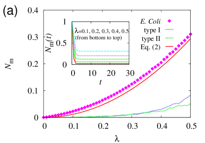
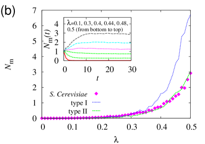
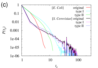
Figure 2: Number of mutated elements $N_{\rm m}(t)$ and $N_{\rm m}=\lim_{t\to\infty}N_{\rm m}(t)$ and distribution of the relaxation time $P(t_{\rm r})$. (a) Plot of the stationary value $N_{\rm m}$ versus $\lambda=2p(1-p)$ in the original network and two types of randomized graphs (see the text for the definition) for E. coli. The data are averages over $10^{2}$ initial pairs of configurations for each of more than $10^{3}$ realizations of regulating rules. The approximation given in Eq. (2) is drawn together. The inset shows the time developments $N_{\rm m}(t)$ for selected values of $\lambda$ in the original E. coli network. (b) The same data as (a) for S. cerevisiae. (c) Plots of $P(t_{\rm r})$ with $p=1/2$ ($\lambda=1/2$) on the original networks and the randomized graphs for E. coli and S. cerevisiae.

III Results

III.1 Time evolution of the number of mutated elements

Figure 2 (a) and (b) present the results for the number of mutated elements $N_{\rm m}(t)$ and $N_{\rm m}$. $N_{\rm m}(t)$ decreases very rapidly from $N_{\rm m}(0)=1$ to a much smaller value for all $p$’s in E. coli. On the other hand, $N_{\rm m}$ for S. cerevisiae increases with time up to a value larger than $1$ for $\lambda\equiv 2p(1-p)\gtrsim 0.42$ ($0.3\lesssim p\lesssim 0.7$) indicating the occurrence of a mutation cascade. Both in E. coli and S. cerevisiae, $N_{\rm m}$ increases with increasing $p$ from $0$ to $1/2$ (or decreasing $p$ from $1$ to $1/2$) since the probability that a regulating rule yields different output values from different input configurations is $2p(1-p)$, which has a maximum at $p=1/2$ and will be denoted by $\lambda$. In E. coli, $N_{\rm m}$ stays smaller than $0.3$, indicating that system-wide mutations are suppressed. Figure 2 also shows that in S. cerevisiae $N_{\rm m}$ is smaller than in E. coli for $\lambda\lesssim 0.2$ but increases with $\lambda$ more rapidly and is larger for $\lambda\gtrsim 0.2$.

The functional form of $P(t_{\rm r})$ for $p=1/2$ in Fig. 2 (c) is strikingly different between E. coli and S. cerevisiae: it is exponential for E. coli and a power-law, $P(t_{\rm r})\sim t_{\rm r}^{-1.5(2)}$, for S. cerevisiae. This long tail of $P(t_{\rm r})$ implies that in the case of S. cerevisiae an element can be mutated and recover even at very late times in the dynamics.

III.2 Mean connectivity

These differences in the mutation spread dynamics may be primarily attributed to a difference in the mean connectivity and can be understood by a mean-field approach derrida86 ; aldana03 : The probability $H(t)=\lim_{N\to\infty}N_{\rm m}(t)/N$ that a randomly chosen node $i$ is mutated at time $t$, also called the Hamming distance, is given in terms of the probability that a regulator of the node $i$ is mutated, which we denote by $\bar{H}(t)$, and the probability that the regulating rule $f_{i}$ yields different output values from different input configurations, $\lambda$, as

$$H(t+1) = \sum_{k_{\rm in}}\lambda(1-(1-\bar{H}(t))^{k})P_{d}(k),$$

$$\bar{H}(t+1) = \sum_{k,q}\lambda(1-(1-\bar{H}(t))^{k})\frac{qP_{d}(k,q)}{\langle q\rangle}.$$ (1)

Here $P_{d}(k,q)$ is the joint probability that a node has in-degree $k$ and out-degree $q$ and is related to the in-degree distribution $P_{d}(k)=\sum_{q}P_{d}(k,q)$. $H(t)$ and $\bar{H}(t)$ evolve towards their stationary values $H$ and $\bar{H}$. Setting $\bar{H}(t+1)=\bar{H}(t)=\bar{H}$ and expanding the second line of Eq. (1) for small $\bar{H}$, one finds $\bar{H}\simeq\bar{H}\lambda\langle kq\rangle/\langle q\rangle-\bar{H}^{2}\lambda\langle k^{2}q\rangle/(2\langle q\rangle)+\mathcal{O}(\bar{H}^{3})$ provided $\langle q\rangle$, $\langle kq\rangle$, and $\langle k^{2}q\rangle$ are all finite. Therefore $\bar{H}$ and $H$ are zero for $\lambda$ smaller than a critical value $\lambda_{c}$ with $\lambda_{c}=1/K$ and $K\equiv\langle kq\rangle/\langle q\rangle$ and non-zero otherwise. The expression $\lambda_{c}=K^{-1}$ for the critical point holds true as long as $K$ is finite. Since the Hamming distance $H$ can be positive only if $K>2$, $N_{\rm m}\simeq HN$ for finite $N$ should be small in E. coli that has the value $K\simeq 1.08$ and can be large, of order $N$, for $\lambda\gtrsim 0.42$ in S. cerevisiae that has $K\simeq 2.35$. Although the Hamming distance is not necessarily of order $N^{-1}$ at $\lambda_{c}$, one finds the value of $\lambda$ for which $N_{\rm m}=1$ very close to the value $K^{-1}\simeq 0.42$ in the latter. The in-degree $k$ and the out-degree $q$ show no significant correlation in the two networks according to our analysis not presented here, that is, $P_{d}(k,q)\simeq P_{d}(k)P_{d}(q)$ , which yields $\langle kq\rangle\simeq\langle k\rangle\langle q\rangle$ and $K\simeq\langle k\rangle$.

III.3 Comparison with randomized networks

Next we studied the same dynamics in two kinds of randomized networks derived from the regulatory networks of E. coli and S. cerevisiae. The first type of randomized graphs (type I) are constructed by the repetition of removing an edge connecting nodes $v_{1}$ and $w_{1}$ and creating a new one between $v_{2}$ and $w_{2}$, where both $v_{1}$ and $v_{2}$ had at least one outward edge and the node pair $v_{2}$ and $w_{2}$ were not connected before this change. Thus these type-I randomized networks have the same number of nodes, edges, and TF’s as the original networks, but the edges connect randomly-chosen pairs of TF and target gene. Our results for $N_{\rm m}$ and $P(t_{\rm r})$ are shown in Fig. 2. For the type-I randomized graphs derived from E. coli, $N_{\rm m}$ is substantially suppressed as compared with the original network. In the type-I random graphs derived from S. cerevisiae, $N_{\rm m}$ increases much more rapidly passing $\lambda\simeq 0.3$. The relaxation time distribution for the random graphs from E. coli is broader than for the original network but still decays faster than that for S. cerevisiae. The type-I randomization does not change significantly the relaxation time distribution for S. cerevisiae.

The type-II randomized graphs we considered are constructed by exchanging the end points of two edges: Two randomly chosen edges $e_{1}=(v_{1},w_{1})$ and $e_{2}=(v_{2},w_{2})$ are replaced by $e_{1}^{\prime}=(v_{1},w_{2})$ and $e_{2}^{\prime}=(v_{2},w_{1})$, respectively. These graphs preserve the joint degree distribution $P_{d}(k,q)$, but their local connectivity patterns may be different from that in the original network. We present the plots of $N_{\rm m}$ and $P(t_{\rm r})$ in Fig. 2. This type-II randomization does not change the relaxation time distribution for S. cerevisiae neither. Thus much faster decay of the relaxation time in the original and randomized networks for E. coli than in those for S. cerevisiae can be ascribed to the much lower mean connectivity, $\langle k\rangle\simeq 1.24$, of the former than that of the latter, $\langle k\rangle\simeq 2.73$. Interestingly the quantities $N_{\rm m}$ and $P(t_{\rm r})$ for these randomized graphs agree well with those for the original network of S. cerevisiae, but not for E. coli: This implies that it is the degree distribution that is mainly responsible for the spread of mutation in S. cerevisiae while other (local) structural factors must be important in E. coli.

Figure 3: Network structure dependence of mutation spread. The regulating rules are given by $f_{i}(\sigma)=\sigma$ or $1-\sigma$ for nodes $i$’s with one input and $f_{i}=1$ or $0$ for nodes $i$’s with no input. Thus a mutated regulator necessarily makes its target node mutated at the next time step. Time evolution of $\Delta\sigma_{i}=|\sigma_{i}-\hat{\sigma}_{i}|$ for each node is shown in tables. (a) No circuit (tree structure). All nodes recover at $t=3$ and thus the Hamming distance $H$ is zero. (b) A circuit of length $3$. The point mutation circulates with period $3$, resulting in $H=1/3$. (c) A single-element circuit together with tree structure. All nodes are mutated at $t=2$ and thus $H=1$.

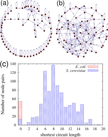
Figure 4: Organization of the core in E. coli and S. cerevisiae. (a) Core of E. coli. It consists of $57$ nodes and $84$ edges. (b) Core of S. cerevisiae. It has $63$ nodes and $167$ edges. (c) Histogram of the shortest circuit lengths. In E. coli, a circuit longer than $1$ is not observed but all $54$ circuits are single-element ones. In S. cerevisiae, $836$ pairs of nodes among all possible $1953$ pairs in the core are connected by circuits and the shortest circuit length ranges from $0$ to $19$.

III.4 Abundance of single-element circuits in E. coli

One might expect that circuits (directed closed paths) in the regulatory network play an important role for the spread of mutations, because in networks with a tree-structure, i.e., without circuits, point mutations spread without circulation and a node that is mutated will recover at the next time step and never become mutated again as indicated in Fig. 3 (a). The nodes on a circuit, on the other hand, can return to a mutated state even after recovery [Fig. 3 (b)]. The nodes lying on circuits or those on bridges connecting distinct circuits can in principle switch their status permanently and thus they can be considered as comprising a core in the dynamics of mutation spread. As a subnetwork including all such circuits and the bridges connecting them, we define the core of a network as the maximal subgraph in which each node has at least one inward edge coming from and at least one outward edge incident to an element of the core.

By deleting the edges having at either end a node that does not meet the requirement for the core elements, we found the core subnetwork in the regulatory networks of E. coli and S. cerevisiae. Note that if an edge has the same node at both ends, the node, which regulates itself, becomes the element of the core. The relevance of the core to the mutation spread dynamics can be understood e.g., by investigating the relaxation time distribution $P(t_{\rm r})$ in S. cerevisiae depending on the location of the initial point mutation. Our analysis shows that initial mutations in the core lead to a qualitatively equal (power-law with the same exponent) distribution of the relaxation time. On the other hand, initial mutations in the output module, consisting of all nodes that have inward edges coming from the nodes in the core and their edges, decay very fast since the output module has a tree structure and cannot cause mutations in the core.

The organization of the core turns out to be very different in E. coli and S. cerevisiae as shown in Fig. 4 (a) and (b), respectively. Most of all, the nodes are much more densely connected in S. cerevisiae than in E. coli. This difference can be first ascribed to different mean connectivities of the nodes in the core: it is about $1.47$ in E. coli and $2.65$ in S. cerevisiae. However, a more striking difference exists in their core organization. In E. coli, all $54$ circuits are identified, all of which are single-element circuits representing self-regulation. There are no circuits whose length (i.e the number of edges on the cycle) is larger than $1$ thieffry98 . On the contrary, only one or two single-element circuits are formed in its randomized graphs. This organization of circuits in E. coli is also contrasted with the one in S. cerevisiae. We computed the shortest circuit for each pair of nodes in the core and counted the numbers of node pairs for each given shortest-circuit length. The distribution of shortest-circuit length obtained for S. cerevisiae is broad as shown in Fig. 4 (c). We propose that the presence of single-element circuits in E. coli is the main reason for the enhancement of $N_{\rm m}$ of E. coli compared with both of its randomized graphs. Once a node $i$ regulating itself is mutated, the input configurations to the regulating rule $f_{i}$ are necessarily different between the normal-mutant pair $(\Sigma,\hat{\Sigma})$ since it is guaranteed that at least one of its regulators, the node $i$ itself, is mutated. Recalling that a node can be mutated at the next time step only if the input configurations from the normal-mutant pair are different, one can see that single-element circuits have a higher probability to be mutated than nodes which do not regulate themselves [See Fig. 3 (c)]. Therefore networks with more single-element circuits can be more adaptive.

In the core of E. coli network, $54$ edges are used for single-element circuits and the remaining $30$ edges connect pairs of distinct nodes. As a result, the network has many isolated nodes and few small connected components, resulting in the rapid decay of the relaxation time. In Fig. 2 (c), we find that the relaxation times observed in E. coli are mostly $1$ or $2$. From this, we can analytically predict the value of $N_{m}$ as a function of $\lambda$. Suppose $N_{\rm m}(t)$ saturates no later than time $2$. From Eq. (1), $\bar{H}(1)=\lambda KN^{-1}+{\cal O}(N^{-2})$ since $\bar{H}(0)=N^{-1}$ and

$$N_{\rm m}\simeq NH(2)\simeq N\lambda K\bar{H}(1)\simeq\lambda^{2}K^{2}.$$ (2)

This is in good agreement with the true value as shown in Fig. 2 (a).

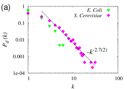
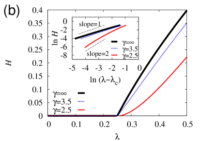
Figure 5: Connectivity pattern and its effect on the critical behavior of the Hamming distance. (a) In-degree distributions $P_{d}(k)$ for E. coli and S. cerevisiae. For S. cerevisiae, its asymptotic behavior is a power-law, $P_{d}(k)\sim k^{-\gamma}$ with $\gamma\simeq 2.7(2)$. On the other hand, the observed values of $k$ are only up to $6$ and so it is hard to discern the functional form of $P_{d}(k)$ in E. coli. (b) Hamming distance $H$ as a function of $\lambda$ numerically obtained from Eq. (3) with $P_{d}(k)$ of the static model lee04 , which has a power-law tail as $P_{d}(k)\sim k^{-\gamma}$ with the exponent $\gamma$ tunable. The inset shows that $H\sim\Delta$ commonly for $\gamma\to\infty$ and $\gamma=3.5$, and that $H\sim\Delta^{2}$ for $\gamma=2.5$, in agreement with Eq. (4).

III.5 Power-law in-degree distribution in S. cerevisiae

In S. cerevisiae, the most significant dynamical feature that we found and that we need to explain is the slower increase of $N_{\rm m}$ with $\lambda$ as compared with the type-I randomized graph, shown in Fig. 2 (b). Contrary to the type-II randomized graphs, those of type-I do not preserve the degree distribution of the original network. From this, we can conjecture that the degree distribution of S. cerevisiae causes the slow increase of $N_{\rm m}$. To check this, we analyze in detail the dependence of the Hamming distance on the degree distributions.

With uncorrelated in- and out-degree as is the case in the regulatory networks considered here, Eq. (1) is reduced to $H(t)=\bar{H}(t)$ and

$$H(t+1)=\lambda\sum_{k}[1-(1-H(t))^{k}]P_{d}(k).$$ (3)

Thus the in-degree distribution $P_{d}(k)$ determines the behavior of the Hamming distance $H(t)$. The in-degree distributions of E. coli and S. cerevisiae shown in Fig. 5 (a) are quite different from each other. The maximum degree is $31$ in S. cerevisiae while it is only $6$ in E. coli. Furthermore, the log-log plot of $P_{d}(k)$ in S. cerevisiae indicates that $P_{d}(k)\sim k^{-\gamma}$ with $\gamma\simeq 2.7(2)$. The functional form of $P_{d}(k)$ for E. coli is hard to determine because of the small range for observable $k$ values. Note that the in-degree distribution of the type-I randomized graphs obey a Poisson distribution, $P_{d}(k)=\langle k\rangle^{k}e^{-\langle k\rangle}/k!$. Let us consider an in-degree distribution which has a power-law tail, i.e., $P_{d}(k)\sim k^{-\gamma}$. Then, we find from Eq. (3) that the Hamming distance in the stationary state behaves as $H\sim\Delta^{\beta}$ for $\lambda$ larger than the critical value $\lambda_{c}$ with $\Delta\equiv\lambda/\lambda_{c}-1$ and the critical exponent $\beta$ given by

$$\beta=\left\{\begin{array}[]{ll}1&(\gamma>3),\\ 1/(\gamma-2)&(2<\gamma<3).\end{array}\right.$$ (4)

The derivation of Eq. (4) is given in Appendix. We restricted the range of $\gamma$ to $\gamma>2$ because the mean connectivity diverges with $\gamma<2$. When the in-degree is subject to a Poisson distribution or an exponentially-decaying distribution, it corresponds to $\gamma\to\infty$ and the critical behavior is the same as that for $\gamma>3$. We present the numerical solution to Eq. (3) in Fig. 5 (b) for $\gamma\to\infty$ (Poisson distribution), $\gamma=3.5$, and $\gamma=2.5$.

The increase of $\beta$ with decreasing $\gamma$ below $\gamma=3$ indicates a difference in the behavior of the Hamming distance near the critical point between networks with $\gamma>3$ and those with $2<\gamma<3$. Suppose we have two networks with a power-law in-degree distribution $P_{d}(k)\sim k^{-\gamma}$: One has $\gamma=3.5$ and the other has $\gamma=2.5$, and both have $\langle k\rangle=4$. Then, in the region $0<\Delta=\lambda/\lambda_{c}-1\ll 1$, the Hamming distance behaves as $H\sim\Delta$ for $\gamma=3.5$ and $H\sim\Delta^{2}$ for $\gamma=2.5$: the former increases more rapidly than the latter in the region $\Delta\ll 1$. Also the region where the Hamming distance remains non-zero but small, e.g., $H\leq 0.05$ is larger with $\gamma=2.5$ than with $\gamma=3.5$: it is given by $\lambda\in(0.25:0.29]$ with $\gamma=3.5$ and $\lambda\in(0.25:0.35]$ with $\gamma=2.5$. Such dependence of the Hamming distance on the in-degree exponent $\gamma$ can thus explain different network responses between S. cerevisiae and its type-I randomized graphs. It is the broad in-degree distribution with $\gamma=2.7(2)$ that makes the number of mutated elements increase with $\lambda$ more slowly than in the corresponding type-I randomized graphs that have $\gamma\to\infty$. Due to such a slow increase of the Hamming distance, S. cerevisiae can keep the size of mutation small for a wider range of the parameter $p$ or $\lambda$, which would be much larger with random structures.

IV Conclusion

We performed numerical experiments - spread of mutation - to probe the dynamic stability of the recently-unveiled networks of gene transcriptional regulation of E. coli and S. cerevisiae and provided analytical confirmation for the results by analyzing their structural features. While the small number of edges per node in E. coli fundamentally prohibits a global spread of mutation, a relatively large number of edges in S. cerevisiae enables a global mutation conditionally depending on the regulating rules. We further identified the relevant structural features which are distinguished from those of random graphs: All circuits of the regulatory network of E. coli are single-element circuits and the in-degree distribution of S. cerevisiae takes a power-law form. Single-element circuits in E. coli have higher probability to be mutated than nodes without self-regulation. The broad in-degree distribution in S. cerevisiae smoothens the increase of the number of mutated elements. This increase would be sharper for an exponential distribution, as is the case in the random graphs.

These biological networks appear to follow design principles that tend to balance the size of mutation. The small mean connectivity of the regulatory network of E. coli would restrict the size of mutations drastically, which is compensated by the abundance of single-element circuits that lead to the required enhancement of the mutation size. In the case of S. cerevisiae, its global characteristics of the regulatory network, a mean connectivity larger than 2, would lead to a very large mutation size, but a very heterogeneous interconnectivity pattern suppresses it. These local structural features demonstrate that both genetic networks have evolved, in spite of the restrictions imposed by the global characteristics, in such a direction that they can stay dynamically between stable (i.e., rarely mutated on a global scale) and unstable (easily mutated). Being neither stable nor unstable appears to be necessary for living organisms to maintain their stable internal state and adapt itself to fluctuating external environment simultaneously. Therefore our finding suggests that such a marginal dynamic stability of the whole system is supported by a selected structural organization of the internal systems on smaller scales, as the transcriptional regulatory network studied in this work. While we have concentrated only on the average in-degree, the organization of circuits, and the in-degree distribution of the network, further structural analysis will be helpful to illuminate how structure supports function.

Appendix A Derivation of Eq. (4) from Eq. (3)

To find the behavior of $H=\lim_{t\to\infty}H(t)$ as a function of $\lambda$ near the critical point $\lambda_{c}=\langle k\rangle^{-1}$, we set $H(t+1)=H(t)=H$ and expand Eq. (3) for small $H$, which leads to

$$H=\lambda\sum_{n=1}^{\infty}\frac{(-1)^{n+1}\langle k^{n}\rangle}{n!}H^{n}.$$ (5)

Here $\langle k^{n}\rangle$ is the $n$th moment of the in-degree distribution $P_{d}(k)$, i.e., $\langle k^{n}\rangle\equiv\sum_{k}k^{n}P_{d}(k)$. It is finite for all $n$ only if $P_{d}(k)$ decays exponentially. In this case, all the terms in the right-hand-side of Eq. (5) are analytic and keeping the first two leading terms, one finds that Eq. (5) is expressed as $H\simeq\lambda\langle k\rangle H-\lambda\langle k^{2}\rangle H^{2}/2$. This allows us to see that $H=0$ for $\lambda<\lambda_{c}=\langle k\rangle^{-1}$ and $H\sim\Delta$ with $\Delta\equiv(\lambda-\lambda_{c})/\lambda_{c}$ for $\lambda>\lambda_{c}$.

When the in-degree distribution is a power-law asymptotically, $P_{d}(k)\sim k^{-\gamma}$, all the moments $\langle k^{n}\rangle$ are not finite: $\langle k^{n}\rangle$ for $n>n_{*}$ with $n_{*}=\lceil\gamma-2\rceil$ diverges as $k_{\rm max}^{n-\gamma+1}/(n-\gamma+1)$, where $\lceil x\rceil$ is the smallest integer not smaller than $x$ and $k_{\rm max}$ is the (average) largest in-degree. The largest in-degree diverges as $N^{1/(\gamma-1)}$, which is derived from the relation $\sum_{k>k_{\rm max}}P_{d}(k)\sim N^{-1}$. Thus $\langle k^{n}\rangle\sim N^{(n-\gamma+1)/(\gamma-1)}$. Such diverging terms are arranged as $H^{\gamma-1}\sum_{n>n_{*}}(-1)^{n+1}[k_{\rm max}H]^{n-\gamma+1}/[n!(n-\gamma+1)]$ in the right-hand-side of Eq. (5). Here the summation converges to a constant in the limit $k_{\rm max}\bar{H}\to\infty$ due to alternating signs and fast decay of the coefficients lee05 . Thus the small-$H$ expansion of Eq. (5) reads as $H=\lambda\sum_{n=1}^{n_{*}}(-1)^{n+1}\langle k^{n}\rangle H^{n}/n!+\lambda({\rm constant})H^{\gamma-1}+\cdots.$. The $H^{\gamma-1}$ term is relevant to the critical behavior of $H$ for $\gamma<3$ since it holds for $\gamma<3$ that $H\simeq\lambda\langle k\rangle H+\lambda({\rm const.})H^{\gamma-1}$, yielding $H\sim\Delta^{1/(\gamma-2)}$. On the other hand, the linear and quadratic terms are relevant for $\gamma>3$ as for exponentially-decaying in-degree distributions. In summary, the Hamming distance $H$ with a power-law in-degree distribution $P_{d}(k)\sim k^{-\gamma}$ behaves near the critical point as

$$H\sim\left\{\begin{array}[]{cc}\Delta&(\gamma>3),\\ \Delta^{1/(\gamma-2)}&(2<\gamma<3).\end{array}\right.$$ (6)

References

- (1) H.C. Causton et al., Mol. Biol. Cell 12 323 (2001).
- (2) M.M. Babu et al. Curr. Opin. Struct. Biol. 14, 283 (2004).
- (3) D. Thieffry, A.M. Huerta, E.Pérez-Rueda, and J. Collado-Vides, Bioessays 20, 433 (1998).
- (4) R. Dobrin, Q.K. Beg, A.-L. Barabási, and Z.N. Oltvai, BMC Bioinformatics 5, 10 (2004).
- (5) S. Shen-Orr, R. Milo, S. Mangan, and U. Alon, Nature Genetics, 31, 64 (2002).
- (6) N. Guelzim, S. Bottani, and F. Képès, Nature Genetics, 31, 60 (2002).
- (7) T. I. Lee et al., Science 298, 799 (2002).
- (8) N.M. Luscombe et al., Nature 431, 308 (2004).
- (9) G. Orphanides and D. Reinberg, Cell 108, 439 (2002).
- (10) N. Buchler, U. Gerland, and T. Hwa, Proc. Natl. Acad. Sci. U.S.A. 100, 5136 (2003).
- (11) S. Kauffman, J. Theor. Biol. 22, 437 (1969); The Origins of Order: Self-organization and Selection in Evolution (Oxford Univ. Press, Oxford, 1993).
- (12) B. Samuelsson and C. Troein, Phys. Rev. Lett. 90, 098701 (2003).
- (13) K. Klemm and S. Bornholdt, Phys. Rev. E 72, 055101 (2005).
- (14) S.E. Harris, B.K. Sawhill, A. Wuensche, and S. Kauffman, Complexity 7, 23 (2002).
- (15) S. Kauffman, C. Peterson, B. Samuelsson, and C. Troein, Proc. Natl. Acad. Sci. U.S.A. 100, 14796 (2003); ibid. 101, 17102 (2004).
- (16) B. Derrida and Y. Pomeau, Europhys. Lett. 1, 45 (1986).
- (17) M. Aldana and P. Cluzel, Proc. Natl. Acad. Sci. 100, 8713 (2003).
- (18) D.-S. Lee, K.-I. Goh, B. Kahng, and D. Kim, Nucl. Phys. B 696, 351 (2004).
- (19) D.-S. Lee, Phys. Rev. E 72 026208 (2005).