Effects of rapid prey evolution on predator-prey cycles

Abstract

We study the qualitative properties of population cycles in a predator-prey system where genetic variability allows contemporary rapid evolution of the prey. Previous numerical studies have found that prey evolution in response to changing predation risk can have major quantitative and qualitative effects on predator-prey cycles, including: (i) large increases in cycle period, (ii) changes in phase relations (so that predator and prey are cycling exactly out of phase, rather than the classical quarter-period phase lag), and (iii) “cryptic” cycles in which total prey density remains nearly constant while predator density and prey traits cycle. Here we focus on a chemostat model motivated by our experimental system [14, 41] with algae (prey) and rotifers (predators), in which the prey exhibit rapid evolution in their level of defense against predation. We show that the effects of rapid prey evolution are robust and general, and furthermore that they occur in a specific but biologically relevant region of parameter space: when traits that greatly reduce predation risk are relatively cheap (in terms of reductions in other fitness components), when there is coexistence between the two prey types and the predator, and when the interaction between predators and undefended prey alone would produce cycles. Because defense has been shown to be inexpensive, even cost-free, in a number of systems [4, 16, 42], our discoveries may well be reproduced in other model systems, and in nature. Finally, some of our key results are extended to a general model in which functional forms for the predation rate and prey birth rate are not specified.

1 Introduction

The potential for rapid evolutionary change is well documented: in some natural and experimental settings, trait evolution and population dynamics are observed to occur on similar time scales [20, 22, 29, 38]. Though laboratory demonstrations of the interactions between trait and population dynamics still remain rare, there are a few direct examples [13, 27] and also examples where these interactions are inferred via modeling (e.g., [10, 41, 43]). Furthermore, documented cases where the effects of rapid evolution are observed in a changing natural environment are increasing (e.g., [5, 12, 17, 19, 21, 28, 32], and for reviews on the topic, [6, 20, 33, 44]). Among the fishes, rapid evolution has been observed or inferred in natural populations of atlantic cod (Gadus morhua), which evolved towards reproductive maturity at earlier ages and smaller sizes under heavy size-dependent selection (fishing) [28]. Within four hatchery generations, Chinook salmon (Oncorhynchus tshawytscha) raised in hatcheries to supplement natural populations evolve life-history traits (smaller eggs) that reduce odds of survival in the wild [21].

Where prey are under strong selection to avoid predation (because the risk of getting eaten is very strong natural selection), prey genetic diversity yields the capacity for rapid evolution of resistance to predation, akin to the rapid evolution of microbial pathogens in response to antibiotics. However, prey defensive strategies, be they physiological, behavioral, or developmental, may themselves exact demographic costs from the prey equivalent to or greater than that of direct consumption by predators [31]. The energetic costs of defense traits in “trait mediated interactions”, for example the development of armored spines in Daphnia when exposed to chemicals from fish, reduce lifetime fitness by routing energy to defense which would otherwise go into progeny [7]. Thus, by focusing exclusively on changes in population numbers without considering changes in the properties (and associated costs) of individuals comprising the populations, conventional models of population and community dynamics may give us, at best, only half the story in a system where prey adapt to predation risk. The capacity for rapid evolution may expand the conditions permitting coexistence of predator and prey. For example, within the ecosystem of the human body, rapid prey evolution may allow viruses (prey) to escape detection by immune cells (predators) by altering a few surface proteins, or allow a pathogenic strain of bacteria to evolve so that it is no longer sensitive to a widely-used antibiotic. Heterogeneity in prey edibility may also shift prey population regulation from top-down to bottom-up by providing a haven from predation in the form of the less edible prey.

Our experimental system is a predator-prey microcosm with rotifers, Brachionus calyciflorus, and their algal prey, Chlorella vulgaris, cultured together in nitrogen-limited, continuous flow-through chemostats. In prior studies, we have shown that coexistence of edible and inedible prey types (genetic variation in the algal prey) allows the prey to evolve in response to temporally variable selection due to predation pressure from the rotifer predator, and nutrient limitation at high prey densities. While our earlier studies did not specifically track changes at the genotypic level, recent work on our system explicitly identifies two competing algal strains, and tracks changes in their densities as the algal population evolves under predation pressure [27]. Evolution in the prey can lead to “evolutionary” cycling [34, 41], where the predator and prey exhibit extended, out-of-phase population cycles (Figure 1A), or in some circumstances, the odd phenomenon of “cryptic cycles”, where the predator alone exhibits regular population cycles but the prey appear to remain in steady state (Figure 1B). In cryptic cycling, densities of edible and inedible prey cycle out of phase with each other, driven by changes in predator abundance, in such a way that total prey density remains nearly constant [43]. These dynamics are not unique to the organisms in this system: we have observed evolutionary cycles in a chemostat system comprised of rotifers cultured with the flagellated algae Chlamydomonus, and cryptic dynamics have been observed in bacteria-phage microcosms [10, 43]. We are motivated here by just these sorts of perplexing experimental results from our system, and by the close match between our experimental data and model simulations.

Understanding the potential effects of rapid evolution on the dynamics of natural ecosystems is critical to predicting how populations will adapt to a changing environment. Populations in the wild today face unprecedented stress from habitat loss or degradation, harvesting pressure, species introductions and climate change. In addition, otherwise well-intentioned attempts at conservation or management often fail to take into account the potential for rapid Darwinian responses to intervention [24]. Thus before conclusions based on laboratory systems or manipulated natural systems are applied to the natural world, we must ask if the conclusions are likely to be robust: are they limited to the special conditions present in the experimental systems, or should we expect to see them in a broad range of conditions in nature? The present contribution is an attempt, using theory, to answer the questions: how general is the phenomenon of evolutionary cycling in predator-prey systems, under what circumstances might these dynamics be observed, and what are the implications of this type of phenomenon for natural systems?

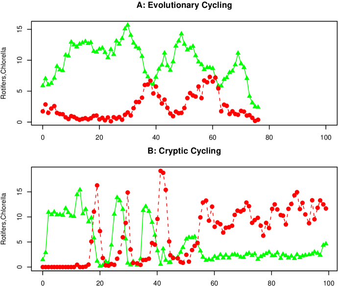
Figure 1: A, “Evolutionary” cycling. Chlorella are shown in solid line, and the rotifer predator is shown dashed. Phase relations are nearly out-of-phase, unlike the quarter-phase shift seen in classic predator-prey cycles. B, Cryptic Cycling. Initially the system exhibits classic predator-prey cycles, which would be expected when a single (edible) prey type is dominant. At about day 50 the system switches to cryptic cycles, which would be expected if a highly defended (inedible) type with low cost for defense arose by mutation. A switch from classic to cryptic cycles when a defended type arises by mutation has been documented in bacteria-phage chemostats [10].

2 The model

Our model is based on an experimental predator-prey microcosm with rotifers, Brachionus calyciflorus, and their algal prey, Chlorella vulgaris, cultured together in a nitrogen-limited, continuous flow-through chemostat system. This system was first described by Fussmann et al. [14], further characterized by Schertzer et al. [34] and Yoshida et al. [41, 42], and equilibrium properties studied by Jones and Ellner [23]. Brachionus in the wild are facultatively sexual, but because sexually produced eggs wash out of the chemostat before offspring hatch, our rotifer cultures have evolved to be entirely parthenogenic [15]. The algae also reproduce asexually [30], so evolutionary change in the prey occurs as a result of changes in the relative frequency of different algal clones.

We use a system of ordinary differential equations to describe the population and prey evolutionary dynamics in the experimental microcosms [41, 23]. Genetic variability and thus the possibility of evolution in the prey is introduced by explicitly representing the prey population as a finite set of asexually reproducing clones. Each clone is characterized by its palatability $p$, which represents the conditional probability that an algal cell is digested rather than being ejected alive, once it has been ingested by a predator [27].

The model consists of three equations for the limiting nutrient and rotifers, plus $q$ equations for $q$ prey clones. In the following equations, $N$ is nitrogen ($\mu$ mol per liter), $C_{i}$ represents concentration of the $i^{th}$ algal clone ($10^{9}$ cells per liter), where $i=1,2,....,q$. Here we limit the number of clones to two, for reasons discussed below. $R$ and $B$ are the fertile and total population densities, respectively, for the predator Brachionus (individuals per liter). Fertile rotifers senesce and stop breeding at rate $\lambda$; all rotifers are subject to fixed mortality $m$. The parameters $\chi_{c},\chi_{b}$ are conversions between consumption and recruitment rates (additional model parameters are defined in Table 1).

$$\frac{dN}{dt} =\delta(N_{I}-N)-\sum_{i=1}^{q}F_{C,i}(N)C_{i}$$ (1)

$$\frac{dC_{i}}{dt} =\chi_{c}F_{C,i}(N)C_{i}-p_{i}F_{b}(C_{i})B-\delta C_{i}$$

$$\frac{dR}{dt} =\chi_{b}\sum_{i=1}^{2}p_{i}F_{b}(C_{i})R-(\delta+m+\lambda)R$$

$$\frac{dB}{dt} =\chi_{b}\sum_{i=1}^{2}p_{i}F_{b}(C_{i})R-(\delta+m)B$$

where

$$F_{c,i}(N)=\rho_{c}N/(K_{c}(p_{i})+N)$$

and

$$F_{b}(C_{i})=GC_{i}/(K_{b}+\sum\limits_{i=1}^{2}C_{i}p_{i})$$ (2)

are functional response equations describing algal and rotifer consumption rates, respectively, and where $\rho_{c}=\omega_{c}\beta_{c}/\epsilon_{c}$. Equation (2) is derived from the predator’s clearance rate G (the volume of water per unit time that an individual filters to obtain food). We assume that clearance rate is a function of the total prey food value:

$$\textbf{G}=\frac{G}{K_{b}+\sum\limits_{i=1}^{2}C_{i}p_{i}}.$$ (3)

That is, lower prey palatability results in the predators increasing their clearance rate, exactly as if prey were less nutritious. We also considered a model in which clearance rate depends only on the total prey density, but it could not be fitted as well to our experimental data on population cycles. Elsewhere [41, 27] we have used a more complicated expression for G in order to fit experimental data more accurately, but using (3) does not change the model’s qualitative behavior.

The cost for defense against predation is a reduced ability to compete for scarce nutrients [42, 23, 27]. We model this by specifying a tradeoff curve

$$K_{c}(p)=K_{c}+\alpha_{2}(1-p)^{\alpha_{1}}.$$ (4)

Here $K_{c}>0$ is the minimum value of the half-saturation constant, $\alpha_{1}>0$ determines whether the tradeoff curve is concave up versus down, and $\alpha_{2}>0$ is the cost for becoming completely inedible ($p=0$).

Table 1: Parameter estimates for the Chlorella-Brachionus microcosm system. Set: adjustable parameters set by the experimenter. TY: Unpublished experimental data (Yoshida et al., in prep.) Fitted: Estimated by numerically optimizing the goodness-of-fit between model output and data on total prey and predator population dynamics from two experiments (originally reported by Fussmann [14]) in which regular cycles occurred.

Parameter	Description	value	Reference
$N_{I}$	Limiting nutrient conc. (suplied medium)	$80\mu$ mol N$/l$	Set
$\delta$	Chemostat dilution rate	variable ($d$)	Set
$V$	Chemostat volume	$0.33l$	Set
$\chi_{c}$	Algal conversion efficiency ($10^{9}$ cells/$\mu$mol N)	0.05	[14]
$\chi_{b}$	Rotifer conversion efficiency	$\approx 54000$ rotifers/$10^{9}$ algal cells	Fitted
$m$	Rotifer mortality	$0.055/d$	[14]
$\lambda$	Rotifer senescence rate	$0.4/d$	[14]
$K_{c}$	Minimum algal half-saturation	$4.3$ $\mu$ mol N $/l$	[14]
$K_{b}$	Rotifer half-saturation	$0.835\times 10^{9}$ algal cells $/l$	TY
$\beta_{c}$	Maximum algal recruitment rate	$3.3/d$	TY
$\omega_{c}$	N content in $10^{9}$ algal cells	$20.0$ $\mu$ mol	[14]
$\epsilon_{c}$	Algal assimilation efficiency	$1$	[14]
$G$	Rotifer maximum consumption rate	$5.0\times 10^{-5}$ $l/d$	TY
$\alpha_{1}$	Shape parameter in algal tradeoff	variable, $\alpha_{1}>0$	Fitted
$\alpha_{2}$	Scale parameter in algal tradeoff	variable, $\alpha_{2}>0$	Fitted

3 Characteristics of the model under simulation

A system of $q>2$ prey types invariably collapses to at most two types in the presence of a predator: either a single clone that outcompetes all others, or a pair of very different clones (one very well defended and the other highly competitive) that together drive all intermediate prey types to extinction [41, 23]. Only the latter case is of interest here, because with a single prey type there is no prey evolution. We thus consider here a system of two extreme prey types in the presence of a predator.

Two system parameters can be experimentally varied: the dilution rate $\delta$ (fraction of the culture medium that is replaced daily) and the concentration of the limiting nutrient in the inflowing medium, $N_{I}$. Fussmann et al. [14] showed that $\delta$ is a bifurcation parameter: in both the real system and the model, the system goes to equilibrium at low dilution rates, limit cycles at intermediate dilution rates, and again to equilibrium at high dilution rates. Further increases in $\delta$ lead to extinction of the predator. Toth and Kot [39] proved that the same bifurcation sequence occurs in chemostat models with an age-structured consumer feeding on an abiotic resource (for our experimental system, this would be rotifers feeding on externally-supplied algae that could not reproduce within the chemostat).

The prey vulnerability parameter $p$ is also a bifurcation parameter. In the following discussion, we define evolutionary cycles as both prey types coexisting and exhibiting long-period cycles (period 20–40 days), with the predator and total prey abundance almost exactly out-of-phase with each other. Predator-prey cycles are shorter (6–12 days), display the classic quarter-period phase offset between predator and prey, and involve one prey type cycling with the predator. In addition, both prey may survive and coexist with the predator at an evolutionary equilibrium, or one prey type may be driven to extinction while the other goes to equilibrium with the predator.

Single prey model

Figure 2A shows the dynamics of the single prey model as a function of prey palatability $p$ and dilution rate $\delta$. Parameters giving single-prey predator-prey cycles are indicated by open circles, and elsewhere the system goes to equilibrium. At low $p$ values (up to 0.4–0.6, depending on the predator conversion efficiency $\chi_{B}$) the system goes to equilibrium at all dilution rates. As $p$ increases there is a bifurcation and short, low amplitude predator-prey cycles are observed, initially for the narrow range of dilution rates. When $p$ is higher, oscillations grow in amplitude and increase very slightly in period, and cycling occurs over a larger range of dilution rates. The cycles always exhibit classic predator-prey phase relations.

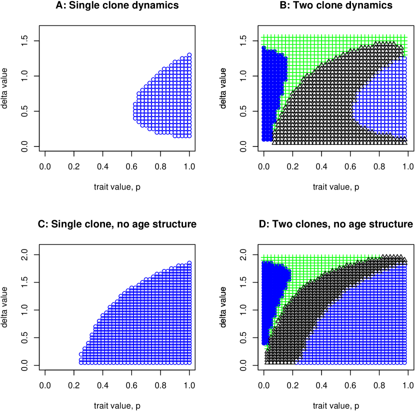
Figure 2: Dynamics of one- and two-prey models as a function of the palatability $p$ of the defended prey type and the dilution rate $\delta$. Panels A and B show results for the “full” model including predator age-structure; panels C and D show results for the “reduced” model without predator age structure. A,C. Dynamics of a single prey system. Open circles show predator-prey cycles, and white space indicates equilibrium. B,D. Dynamics of a two-prey system. The model is scaled so that the undefended prey type has $p=1$. Filled circles indicate that both types coexist and cycle together. Open circles show short predator-prey cycles with only the defended type ($p<1$). Cross-hatching indicates the defended and undefended prey coexisting at a stable equilibrium. Open triangles indicate equilibrium between predator and defended prey and white space indicates equilibrium between predator and vulnerable type. In the model with age structure (panel B), predator extinction occurs for $\delta>1.5$

.

Two prey models

Figure 2B shows dynamics of the two prey model as a function of the dilution rate $\delta$ and the trait value $p$ of the defended prey type (the model is scaled so that the undefended type has $p=1$). Using the parameter values listed in Table 1, extended evolutionary cycles (closed circles) initially appear for all dilution rates ($0.2\leq\delta\leq 1.3$ at $p_{1}$ very small ($p_{1}\approx 0.01$). As $p_{1}$ increases, evolutionary cycling occurs for a diminishing range of dilution rates. By $p_{1}\doteq 0.2$, cycling vanishes and instead the defended prey is in equilibrium (Figure 2B , white space) or the two prey types are in an evolutionary equilibrium with the predator (Figure 2B , crosshatching). As $p_{1}$ increases further ($0.4<p_{1}<0.6$), there is another bifurcation and the system, comprised of the defended type and the predator, begins to exhibit predator-prey cycles (Figure 2B, open circles). From this point on the system behaves as if it were dominated by the defended type (see above), until $p_{1}$ has increased to the point that the two prey types are almost identical. At that point there are predator-prey cycles with both prey types present (closed circles) but these appear to be very long transients rather than indefinite coexistence: one or the other prey type, depending on the dilution rate, is slowly driven to extinction by its competitor.

Eliminating predator age structure

Panels C and D in Figure 2 shows model dynamics without age structure in the predator. Age structure is removed by setting $\lambda=0$ in (1), with all other parameters unchanged. As seen in Figure 2C, the single prey model without age structure exhibits dynamics very similar to those in 2B, where age structure is included. Predator age structure is generally stabilizing in this model because senescent rotifers are a resource sink, eating prey without converting them to offspring. This effect is most pronounced at low values of $\delta$ because senscent rotifers then spend more time in the chemostat before getting washed out. Omitting age structure is therefore destabilizing: it permits cycles with better defended prey (lower $p$) and eliminates entirely the stability at very low $\delta$ for nearly all $p$ values. Similarly, simulations of the two-prey model show that eliminating predator age structure shifts the region of ($p,\delta$) values giving evolutionary cycles to higher dilution rates, and eliminates the stabilization at very low $\delta$, but otherwise the bifurcation diagram is unchanged. Given these similarities in model behavior, we may simplify model (1) by eliminating predator age-structure without changing the properties of interest for this paper.

4 Rescaling the model

We now simplify the model (1-2) by rescaling and further reducing its order. Based on the simulation results above we omit age structure in the predator, which is now represented by the one state variable $B$. We also assume that predator mortality $m$ is negligibly small relative to washout at the dilution rates $\delta$ of interest, and set $m=0$. The model then becomes:

$$\frac{dN}{dt} =\delta(N_{I}-N)-\rho_{c}\sum_{i=1}^{2}\frac{NC_{i}}{K_{c}(p_{i})+N}$$ (5)

$$\frac{dC_{i}}{dt} =C_{i}\left[\chi_{c}\rho_{c}\frac{N}{K_{c}(p_{i})+N}-\frac{Gp_{i}B}{(K_{B}+\sum p_{i}C_{i})}-\delta\right]$$

$$\frac{dB}{dt} =B\left[\chi_{b}\frac{G\sum p_{i}C_{i}}{K_{B}+\sum p_{i}C_{i}}-\delta\right].$$

We order the prey types so that $p_{1}$ and $p_{2}$ correspond to the defended and vulnerable prey types, respectively, $p_{1}<p_{2}$. The cost for defense is reduced ability to compete for scarce nutrients, so $K_{c}(p_{1})>K_{c}(p_{2})$.

To rescale the model we make the following transformations:

$$S=\frac{N}{N_{I}},\quad x_{i}=\frac{C_{i}}{\chi_{c}N_{I}},\quad y=\frac{B}{\chi_{c}\chi_{b}N_{I}},\quad g=\frac{\chi_{b}G}{\delta},\quad m=\frac{\chi_{c}\rho_{c}}{\delta},\quad k_{b}=\frac{K_{B}}{\chi_{c}N_{I}}.\quad\tau=\delta t$$ (6)

The half-saturation constants for each of the two prey types are transformed as follows,

$$k_{1}=K_{c}(p_{1})/{N_{I}},\quad k_{2}={K_{c}(p_{2})}/{N_{I}}.$$ (7)

Substituting these into (5) gives:

$$\dot{S} =1-S-S\sum_{i=1}^{2}\frac{mx_{i}}{k_{i}+S}$$ (8)

$$\dot{x}_{i} =x_{i}\left[\frac{mS}{k_{i}+S}-\frac{gp_{i}y}{(k_{b}+Q)}-1\right]$$

$$\dot{y} =y\left[\frac{gQ}{k_{b}+Q}-1\right]$$

where

$$Q=p_{1}x_{1}+p_{2}x_{2}.$$ (9)

Table 2 gives values of the rescaled model parameters corresponding to the parameter estimates in Table 1.

Table 2: Estimates of rescaled model parameters for the Chlorella-Brachionus microcosm system.

Parameter	Description	Value
$m$	Algal maximum per-capita population growth rate	3.3/$\delta$
$k_{1},k_{2}$	Algal half-saturation constants for nutrient uptake	0.054
$g$	Predator maximum grazing rate	2.55/$\delta$
$k_{b}$	Predator half-saturation constant for prey capture	0.21

We can reduce the dimension of the system further by letting $\Sigma=S+x_{1}+x_{2}+y.$ From (8) we have $\dot{\Sigma}=1-\Sigma,$ so $\Sigma(t)\rightarrow 1$ quickly as $t\rightarrow\infty.$ Thus, to study the long-term dynamics of (8), we may consider the dynamics on the invariant set $\Sigma\equiv 1.$ Then $S(t)=1-x_{1}(t)-x_{2}(t)-y(t)$, and (8) reduces to

$$\dot{x}_{i} =x_{i}\left[\frac{m(1-X-y)}{k_{i}+(1-X-y)}-\frac{gp_{i}y}{(k_{b}+Q)}-1\right],\quad i=1,2$$ (10)

$$\dot{y} =y\left[\frac{gQ}{k_{b}+Q}-1\right]$$

where $X=x_{1}+x_{2}.$

5 Analysis

Our goals in this section are to find the conditions under which two prey types can coexist, to determine when coexistence is steady-state versus oscillatory, and to characterize the period of cycles and the phase relations during oscillatory coexistence and during transients when one type is decreasing to extinction. Throughout this section we consider the reduced model (10). For local stability analysis it is useful to note that the model has the form

$$\dot{x}_{i}=x_{i}r_{i}(x_{1},x_{2},x_{3})\quad i=1,2,3$$ (11)

with $x_{3}=y$. It follows that at any equilibrium where the $x_{i}$ are all positive (and hence the $r_{i}$ are all 0) the Jacobian matrix $J$ has entries

$$J(i,j)=\tilde{x}_{i}\frac{\partial\tilde{r}_{i}}{\partial x_{j}}$$ (12)

with the tilde indicating evaluation at the equilibrium with all $x_{i}$ present. It is also useful for local stability analysis that the determinant of (12) is always negative unless $p_{1}=p_{2}$ (Appendix D).

5.1 Dynamics of a one-prey system

We need first some properties of the one-prey model

$$\dot{x} =x\left[\frac{m(1-x-y)}{k+(1-x-y)}-\frac{gpy}{(k_{b}+px)}-1\right]$$ (13)

$$\dot{y} =y\left[\frac{gpx}{k_{b}+px}-1\right].$$

This is a standard predator-prey chemostat model and its behavior is well-known, so we summarize here only the results that we will need later; see e.g. [36] for derivations and details.

In the absence of predators, the steady state for this system is $E_{0}=(1-\Lambda,0),$ where

$$\Lambda=\frac{k}{m-1}.$$ (14)

$\Lambda$ is the scaled concentration of limiting nutrient at which prey growth balances washout rate, so that $\dot{x}=0.$ Similarly, steady state densities for each prey type in a predator-free two clone system are

$$E_{i}=(1-\Lambda_{i},0)\quad\textrm{where}\quad\Lambda_{i}=\frac{k_{i}}{m-1}.$$

The steady state for the prey in the presence of the predator is

$$\bar{x}_{c}=\frac{k_{b}}{p(g-1)};$$ (15)

$\bar{x}_{c}$ is the prey density at which the predator birth and death rates are equal. The model (13) has an interior equilibrium point $E_{c}=(\bar{x}_{c},\bar{y}_{c})$ representing predator-prey coexistence if

$$\Lambda+x_{c}<1$$ (16)

[36], and otherwise the predator cannot persist. The system then collapses to the prey by itself and converges to $E_{0}$. Condition (16) says that there is an interior equilibrium if the prey by themselves reach a steady state ($1-\Lambda$) that provides enough food so that the predator birth rate exceeds the predator death rate.

The expression for the steady state of the predator, $y_{c}$, is easily obtained from (13):

$$\bar{y}_{c}=\bar{\sigma}-\bar{x}_{c},\quad\mbox{where}\quad\bar{\sigma}=(\bar{x}_{c}+\bar{y}_{c})=\frac{1}{2}\left[\gamma-\sqrt{(\gamma^{2}-4m\bar{x}_{c})}\right],$$ (17)

with $\gamma=k+1+m\bar{x}_{c}$. Similarly, the steady-state densities for the predator in a single-prey system with either prey type, $\bar{y}_{i}$, are found by substituting the steady state for the prey, $\bar{x}_{i}$, in place of $\bar{x}_{c}$ and the appropriate half-saturation $k_{i}$ in place of $k$ in (17).

We can use (16) to derive the condition for predator-prey coexistence in terms of the prey defense trait $p$ and the dilution rate $\delta$, recalling that $\Lambda$ and $x_{c}$ are both implicit functions of $\delta$. Using (14) and (15) we obtain from (16)

$$\frac{k}{m(\delta)-1}+\frac{k_{b}}{pg(\delta)-1}<1,\quad\textrm{or}\quad p>\frac{1}{1-\Lambda}\left(\frac{k_{b}}{g(\delta)-1}\right).$$ (18)

The quantity within parenthesis above is the amount of substrate present in perfect food (undefended prey with $p=1$). Solving (18) for $\delta$ in terms of $p$ yields the boundary between predator extinction and stable coexistence in Figure 3. To the left of this line, the predator goes extinct and the equilibrium is $E_{0}$. As the left-hand side of the second expression in (18) is an increasing function of $p$, and the right-hand side is an increasing function of $\delta$, the range of $p$ values yielding coexistence narrows as $\delta$ increases (see Figure 3).

As in the standard Rosenzweig-MacArthur predator-prey model, the stability condition has a graphical interpretation in terms of the nullclines. The prey nullcline is a parabola which peaks at

$$x^{*}=\frac{1}{m}\left[1-k+\sqrt{\Lambda}(m-2)\right].$$

The coexistence equilibrium is locally unstable if the peak of the prey nullcline is to the right of the predator nullcline (i.e., if $x^{*}>\bar{x}_{c}$). Note that a system with defended prey ($p<1$) is always more stable than a system with fully vulnerable prey ($p=1$) as reductions in $p$ shift the predator nullcline to the right.

From (12) the Jacobian of (13) at $E_{c}$ has the form

$$J_{c}=\begin{bmatrix}\bar{x}_{c}\frac{\partial\bar{r}_{1}}{\partial x}&-\\ +&0\\ \end{bmatrix}$$ (19)

so $E_{c}$ is locally stable if the trace Tr$(J_{c})=\bar{x}_{c}\frac{\partial\bar{r}_{1}}{\partial x}$ is negative. Cycles emerge through a Hopf bifurcation when the trace becomes positive. The condition Tr$(J_{c})\geq 0$ is equivalent to the following expression for model (13):

$$\frac{mk}{(k+1-\bar{x}_{c}-\bar{y}_{c})^{2}}\geq\frac{gp^{2}\bar{y}_{c}}{(k_{b}+p\bar{x}_{c})^{2}}$$ (20)

[36]. Cycles begin when the rates of change in prey substrate uptake (LHS) and in predator consumption (RHS) with respect to the amount of substrate present as prey ($x$) are exactly equal. Numerically solving (20) for $\delta$ in terms of $p$ yields the boundary between stable coexistence and predator-prey cycles in Figure 3. It is known that these cycles are stable and unique near the Hopf bifurcation, and numerical evidence uniformly indicates that they are always unique and attract all interior initial conditions except $E_{c}$ [36].

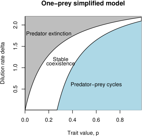
Figure 3: Bifurcation diagram for the rescaled, reduced clonal model with one prey type.

.

5.2 Stability and dynamics of a two-prey system

System (10) has two prey types ordered so that $0<p_{1}<p_{2}=1$. We refer to prey 1 as the defended type and prey 2 as the vulnerable type. The cost for defense comes in the form of reduced growth rate, $1/k_{1}\leq 1/k_{2}$.

Following Abrams [3], we begin by finding the conditions for existence of an equilibrium $(\tilde{x}_{1},\tilde{x}_{2},\tilde{y})$ at which all three population densities are positive; we refer to this as a coexistence equilibrium. Setting (10) to zero and solving gives expressions for $\tilde{X},\tilde{Q}$ and $\tilde{y}$ in terms of model parameters (see Appendix C; as above $Q=p_{1}x_{1}+p_{2}x_{2}$ is the total prey quality, and $X=x_{1}+x_{2}$ is the total prey density). The prey steady states $\tilde{x}_{1},\tilde{x}_{2}$ are then

$$\left[{\begin{array}[]{*{20}c}\tilde{x}_{1}\\ \tilde{x}_{2}\\ \end{array}}\right]=\frac{1}{p_{2}-p_{1}}\left[{\begin{array}[]{*{20}c}p_{2}\tilde{X}-\tilde{Q}\\ \tilde{Q}-p_{1}\tilde{X}\\ \end{array}}\right].$$ (21)

where

$$\tilde{Q}=\frac{k_{b}}{g-1}.$$ (22)

A coexistence equilibrium thus exists provided $\tilde{X}>0$ and $p_{1}\tilde{X}<\tilde{Q}<p_{2}\tilde{X}$, or

$$p_{1}<\frac{\tilde{Q}}{\tilde{X}}<p_{2}.$$ (23)

Beyond the above, system (10) does not yield tidy analytical solutions for the steady states at coexistence. To study how parameter variation affects coexistence, we start by graphically mapping the region where a coexistence equilibrium exists as a function of the defended clone’s parameters, $p_{1}$ and $k_{1}$ (Figure 4), without regard to whether or not the equilibrium is locally stable. The coexistence region also varies with $\delta$, but selecting several $\delta$ values of interest gives a general sense of how the coexistence region varies as a function of dilution rate.

The lower boundary of the coexistence region occurs when the cost of defense is so high that the equilibrium density of the defended prey $x_{1}$ drops to zero while $x_{2}$ and $y$ remain positive. Recalling the general form (11), the lower boundary is thus defined by the conditions

$$r_{1}(0,x_{2},y)=r_{2}(0,x_{2},y)=r_{3}(0,x_{2},y)=0\mbox{ with }x_{2}>0,y>0.$$

The conditions on $r_{2}$ and $r_{3}$ are solved by the steady state $E_{2}=(0,\bar{x}_{2},\bar{y}_{2})$ for a one-prey system with only the vulnerable prey. The lower boundary of the coexistence region is thus defined by the condition $r_{1}(0,\bar{x}_{2},\bar{y}_{2})=0$, which can be written as

$$\frac{1}{k_{1}}=\frac{1}{1-\bar{x}_{2}-\bar{y}_{2}}\left[\frac{\bar{y}_{2}p_{1}+\bar{x}_{2}}{\bar{x}_{2}(m-1)-\bar{y}_{2}p_{1}}\right].$$ (24)

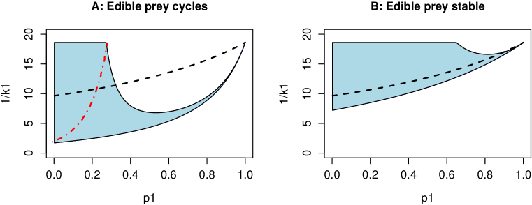
Figure 4: Prey coexistence equilibria. The shaded gray regions indicate parameters $(p_{1},1/k_{1})$ for prey type 1 giving a coexistence equilibrium (stable or unstable) with the vulnerable prey type $p_{2}=1$. At $\delta=1.5$ (panel A) prey type 2 cycles, and at $\delta$ = 2.0 (panel B), prey type 2 is stable. The dashed lines show a representative tradeoff curve (4), assuming roughly 50% reduction in growth rate as the cost of being 100% defended. Here $k_{c}=0.017$, $a_{1}=1.0$, and $a_{2}=0.0165$. In panel A the dash-dotted line indicates where the defended type can invade the limit cycle of the predator and vulnerable prey type.

The upper boundary of the coexistence region occurs when the cost of defense is so low that the defended prey (at the equilibrium density) drives one of the other populations to extinction. In section 6 we show that for $p_{1}<p^{*}=\tilde{Q}/(1-\Lambda_{2})$, the predator goes extinct first ($\tilde{y}\to 0$) as $k_{1}$ decreases, because the defended prey (at steady state) drives the vulnerable prey to low abundance and the defended prey is very poor food. This occurs at $k_{1}=k_{2}$ (zero cost of defense). For $p_{1}>p^{*}$, the vulnerable prey type is outcompeted by the defended type before $k_{1}$ has reached $k_{2}$. This boundary is therefore defined by the conditions

$$r_{1}(x_{1},0,y)=r_{2}(x_{1},0,y)=r_{3}(x_{1},0,y)=0\mbox{ with }x_{1}>0,y>0.$$

The conditions on $r_{1}$ and $r_{3}$ are solved by the one-prey steady state $E_{1}=(\bar{x}_{1},0,\bar{y}_{1})$, so the condition $r_{2}(\bar{x_{1}},0,\bar{y_{1}})=0$ defines the upper boundary of the coexistence region for $p>p^{*}$. The upper boundary of the coexistence region is thus the curve

$$\frac{1}{k_{1}}=\textrm{min}\left[\frac{1}{k_{2}},\frac{1}{\varphi(\bar{x}_{1},\bar{y}_{1})}\right]$$ (25)

where $\varphi$ is value of $k_{1}$ that solves

$$\frac{m(1-\bar{x}_{1}-\bar{y}_{1})}{k_{2}+(1-\bar{x}_{1}-\bar{y}_{1})}-\frac{\bar{y}_{1}+p_{1}\bar{x}_{1}}{(p_{1}\bar{x}_{1})}=0,$$ (26)

noting that $\bar{x}_{1}$ and $\bar{y}_{1}$ are functions of $k_{1}$ and $p_{1}$. The two segments of the upper boundary defined by (25) meet at the point

$$p_{1}=p^{*}=\frac{\bar{Q}}{1-\Lambda_{2}},\quad k_{1}=k_{2}.$$

As $\delta\to 0$ (with the parameter scalings in Table 2), $\bar{Q}\downarrow 0$ and $\Lambda_{2}\uparrow 1$, so $p^{*}\uparrow 0$ so there is typically an increasingly narrow band of $p_{1}$ values for which a $p_{1}--k_{1}$ tradeoff curve lies in the coexistence equilibrium region (unless the tradeoff curve happens to lie exactly inside the cusp of the coexistence equilibrium region).

As $p_{1}\rightarrow 1$, the upper and lower boundaries of the coexistence region meet at $p_{1}=p_{2}=1,k_{1}=k_{2}$ (Figure 4). That is, if the two prey are almost equally vulnerable to predation, they can only coexist at equilibrium if a tiny bit of defense has a tiny cost. To prove that this occurs, we show that the point $p_{1}=1,k_{1}=k_{2}$ lies on both boundaries. At this point the two prey are identical so $\bar{x}_{1}=\bar{x_{2}}$ and $\bar{y}_{1}=\bar{y}_{2}$. The upper boundary is defined by $r_{2}(\bar{x}_{1},0,\bar{y}_{1})=0$. At $p_{1}=1,k_{1}=k_{2}$,

$$r_{2}(\bar{x}_{1},0,\bar{y}_{1})=r_{2}(\bar{x}_{2},0,\bar{y}_{2})=r_{2}(0,\bar{x}_{2},\bar{y}_{2})=0,$$

thus $p_{1}=1,k_{1}=k_{2}$ lies on the upper boundary. The lower boundary is defined by $r_{1}(0,\bar{x}_{2},\bar{y}_{2})=0$. At $p_{1}=1,k_{1}=k_{2})$,

$$r_{1}(0,\bar{x}_{2},\bar{y}_{2})=r_{1}(0,\bar{x}_{1}\bar{y}_{1})=r_{2}(\bar{x}_{1},0,\bar{y}_{1})=0,$$

which shows that $p_{1}=1,k_{1}=k_{2}$ lies on the lower boundary. Thus both boundaries converge to $k_{1}=k_{2}$ as $p_{1}\to 1$.

5.3 Local stability of coexistence equilibria

To characterize two-prey evolutionary cycles we need to find the bifurcation curves in parameter space where these cycles arise. The “empirical facts” are summarized in Figure 5, based on numerical evaluations of the Jacobian and its eigenvalues within the coexistence equilibrium region. In Figure 5 we change the stability of the (predator + vulnerable prey) system by varying the value of $\delta$, but the results are qualitatively the same if other parameters are varied instead (e.g., varying the prey maximum growth rates).

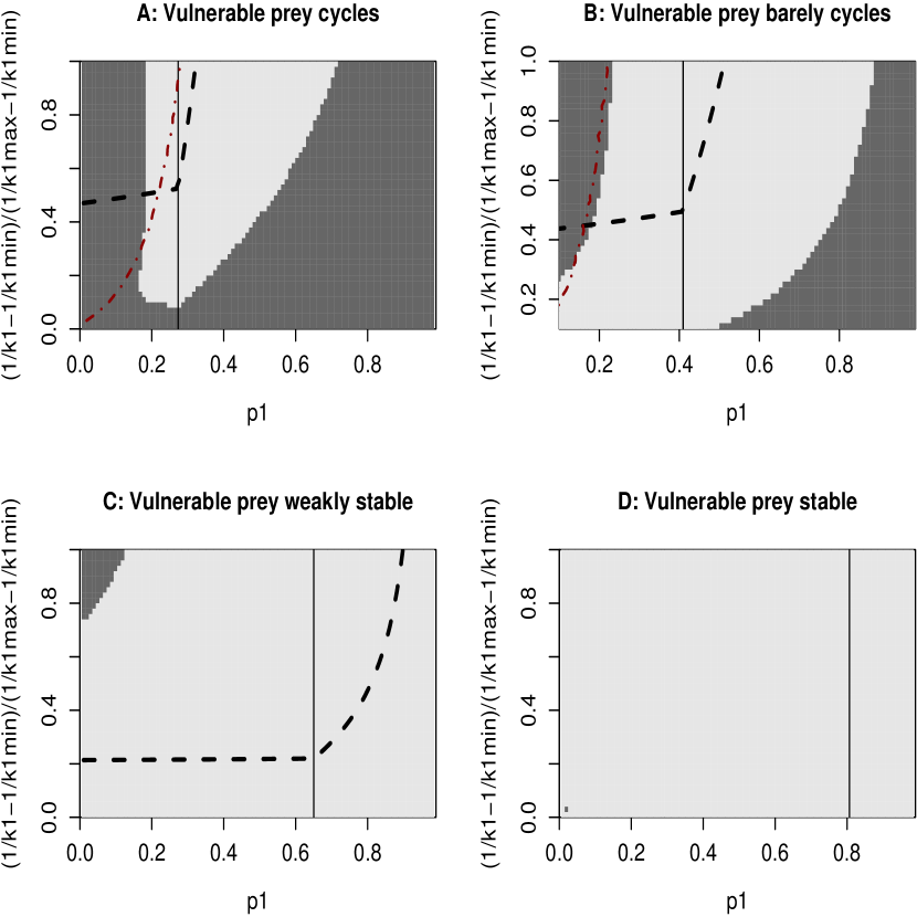
Figure 5: Stability of coexistence equilibria for the reduced two-prey model. In each panel, the horizontal axis is the palatability $p_{1}$ of the defended prey with the model scaled so that $p_{2}=1$. To remain consistent with Abrams (cf. [3], Figures 1 - 3) the vertical axis is $1/k_{1}$, scaled so that 0 and 1 correspond to the lower and upper limits of the coexistence equilibrium region (Figure 4). The Jacobian matrix and its eigenvalues were evaluated at an even $50\times 100$ grid of values. Lighter gray indicates that the equilibrium is stable, darker gray that it is unstable; in all cases the computed eigenvalues with largest real part are a complex conjugate pair. The vertical black line is at $p_{1}=p^{*}$, the value where the straight and curved segments of the upper limit of the coexistence equilibrium region meet. The dashed curve in panels A and B is the tradeoff curve $k_{1}=k_{c}+\alpha_{2}(1-p_{1})^{\alpha_{1}}$, with $k_{c}=k_{2}=0.054,\alpha_{1}=1;\alpha_{2}=0.05$ at $p_{1}$ values lying within the coexistence equilibrium region. The dash-dotted line represents the minimum $1/k_{1}$ values at which the defended prey can invade the (predator + vulnerable prey) limit cycle (see Appendix E). Parameter values for these plots are as follows: panel A., $\delta=1.5$; B., $\delta=1.75$; C., $\delta=2.0$ and D., $\delta=2.1$. All other parameters are unchanged and are as shown in Table 2.

The stability properties in Figure 5 explain the major qualitative features of the two-prey model’s bifurcation diagram (Figure 2D). To see the connection, recall that a horizontal (constant $\delta$) slice through Fig. 2D corresponds to a tradeoff curve between $p_{1}$ and $k_{1}$ in the panel of Figure 5 with the same value of $\delta$. Panel A of Figure 5 has $\delta=1.5$. When $p_{1}$ is near 1, the tradeoff curve lies above the coexistence equilibrium region, and the defended prey type eventually outcompetes the vulnerable type. For $p_{1}$ very close to 1 the prey types are very similar, and the vulnerable type persists for a long time. The system exhibits “classical” predator-prey cycles as if a single prey-type were present, even though two types are transiently coexisting. For $p_{1}$ somewhat smaller, the vulnerable type is quickly eliminated and there are either classical cycles with only the defended type (open circles in Fig. 2D), or (for lower values of $p_{1}$) the defended prey type goes to a stable equilibrium with the predator (open triangles in Fig. 2D). As $p_{1}$ decreases further, Figure 5A shows that the tradeoff curve enters the coexistence region in the area where the coexistence equilibrium is stable, so the system then exhibits stable coexistence (cross-hatching in Fig. 2D). Finally, as $p_{1}$ decreases towards 0, the tradeoff curve enters the area where the coexistence equilibrium is unstable, and it lies above the dash-dot curve marking the $k_{1}$ value required for the defended prey type to invade the vulnerable prey’s limit cycle with the predator. The system exhibits evolutionary cycles with both prey types persisting (filled circles at $p\approx 0$ in Fig. 2D).

Figure 5A also shows that there is a region of parameters (below the dash-dot curve) where the coexistence equilibrium is stable and the system therefore has coexisting attractors: a locally stable coexistence equilibrium, and a locally stable limit cycle with the predator and the vulnerable prey.

Figure 5B, which has $\delta=1.75$, shows the same sequence of transitions as Figure 5A, but each occurs at higher values of $p_{1}$, reflecting the stabilizing effect of increased washout. This is reflected in Figure 2D: increasing $\delta$ above 1.0 shifts all the bifurcation boundaries to higher $p$ values, but the sequence of bifurcations as $p$ decreases is unchanged. However for $\delta$ sufficiently high (panels C and D in Figure 5), the tradeoff curve lies either below the coexistence equilibrium region or within the region where the coexistence equilibrium is stable, so evolutionary cycles never occur. Instead, there is either stable coexistence of the two prey with the predator, or classical predator-prey cycles with only the vulnerable prey type.

Evolutionary cycles are also eliminated – but for a different reason – as $\delta\downarrow 0$ in Figure 2D. As noted above, as $\delta\downarrow 0$ we also have $p^{*}\downarrow 0$, so unless $p_{1}\approx 0$ the tradeoff curve lies above the coexistence equilibrium region and only the defended prey persists with the predator, cycling at higher $p_{1}$ and stable at lower $p_{1}$. Only very near $p_{1}=0$, a region tiny enough to be missed by our simulation grid in Figure 2, can there be coexistence of both prey with the predator.

Stability on the edges.

We can gain some understanding of the patterns in Figure 5, and see that they are not specific to the parameter values used to draw the Figure, by examining the limiting cases that occur along the edges of the coexistence equilibrium region. One general conclusion (explained below) is that the bottom and right edges, and the right-hand portion of the top edge, all must have the same stability as the reduced system with the predator and only the vulnerable prey (prey type 2). However even if this system is unstable, there must be a region along the top edge where the coexistence equilibrium is stable.

The Jacobian matrix that determines equilibrium stability is derived in Appendix D. We also show there that the determinant of this Jacobian is always negative at a coexistence equilibrium unless $p_{1}=p_{2}$, so the coefficient $c_{0}=-\det(J)$ in the Routh-Hurwitz stability criterion for 3-dimensional systems is always positive.

Bottom and right edges:

Near the bottom and right edges, the coexistence equilibrium has the same local stability as the (predator + vulnerable prey) subsystem (panels A and B versus C and D in Fig 5). The bottom edge is the lower limit of the coexistence equilibrium region, where $\tilde{x}_{1}\to 0.$ The coefficients for the Routh-Hurwitz stability criterion (see Appendix B) are then

$$c_{0}=-\det(J)>0,\quad c_{1}=T_{2}(J)\to\delta_{2},\quad c_{2}=-T(J)\to-\tau_{2}$$ (27)

where $\delta_{2}$ and $\tau_{2}$ are the determinant and trace, respectively, of the $2\times 2$ Jacobian for the (predator + vulnerable prey) system. If this one-prey system is stable then $\delta_{2}>0,\tau_{2}<0$ so $c_{0},c_{1}$ and $c_{2}$ are all positive. Moreover $c_{0}=\emph{O}(\tilde{x}_{1})$ (see Appendix D), so when $\tilde{x}_{1}$ is small we have $c_{1}c_{2}>c_{0}$ and the equilibrium is stable. Conversely if the steady state for the (predator + vulnerable prey) system is unstable, $c_{2}$ is negative so the full system is also unstable.

The right edge corresponds to the cusp in the coexistence region as $p_{1}\to 1$. Near the cusp the two prey become increasingly similar ($p_{1}\approx p_{2}=1,k_{1}\approx k_{2}$). Using (12), the functional forms of the $r_{i}$ and the fact that $p_{1}\approx p_{2}$ then imply that the form of $J$ is approximately

$$J_{0}=\left[{\begin{array}[]{*{20}c}{aq}&{aq}&{-qb}\\ {a(1-q)}&{a(1-q)}&{-(1-q)b}\\ c&c&0\\ \end{array}}\right]$$ (28)

where $q=\tilde{x}_{1}/(\tilde{x}_{1}+\tilde{x}_{2})$; even if $p_{1}$ is near $p_{2}$, it is not necessarily the case that $\tilde{x}_{1}$ is close to $\tilde{x}_{2}$. In (28) $b$ and $c$ are positive while $a$ has the sign of $\partial r_{1}/\partial x_{1}$ which may be positive or negative. One eigenvalue of $J_{0}$ is 0, corresponding to the dynamics of $x_{1}-x_{2}$. The others are $\frac{1}{2}(a\pm\sqrt{a^{2}-4bc}),$ which are also the eigenvalues of a single-prey system at the coexistence steady state. Thus, the two-prey system with $p_{1}\approx p_{2}=1$ “inherits” two eigenvalues from the one-prey system with $p=1$.

When the one-prey system with p=1 is cyclic, the inherited eigenvalues are a complex conjugate pair. In the corresponding eigenvectors, the components for the two clones are identical when $p_{1}=p_{2}$. This implies that when $p_{1}\approx p_{2}$ the eigenvector components will be similar, so the two prey types cycle almost exactly in phase. The period of these oscillations is determined by the inherited eigenvalues, so it is close to the period of the corresponding one-prey system.

When the one-prey system is stable, the Routh-Hurwitz criterion (Appendix B), using $J_{0}$ to approximate trace$(J)$ and $T_{2}(J)$ and the fact that $\textrm{det}(J)<0$ for $p_{1}\not=p_{2}$ , implies that the full system will also be stable. Therefore, a coexistence equilibrium with two nearly identical prey has the same stability as the equilibrium for the corresponding one-prey systems. During damped oscillations onto a stable coexistence equilibrium, or diverging oscillations away from an unstable one, the clones will oscillate nearly in phase with each other and inherit the cycle period of the one-prey system.

Top edge:

The rightmost portion of the top edge also corresponds to the cusp in the coexistence equilibrium region, so the stability here is also the same as that of the (predator + vulnerable prey) system. In general, as $1/k_{1}$ approaches the upper limit of the coexistence equilibrium region when $p_{1}>p^{*}$ (the curved portion), the stability of the two-prey system approaches that of the (predator + defended prey) system with $1/k_{1}$ approaching $1/k_{2}$. This must be stable if the (predator + vulnerable prey) system is stable, because the defended prey is always more stable, as noted above. If the (predator + vulnerable prey) system cycles, then there will be instability as $p_{1}\to 1$ along the top edge.

However, there is always stability near the top edge for $p_{1}\to p^{*}$, as follows. Along the straight portion of the top edge ($p_{1}<p^{*}$), as $1/k_{1}$ approaches the edge, the coexistence equilibrium converges to a limit with $\tilde{y}=0$, while along the curved portion the limiting coexistence equilibrium has $\tilde{x}_{2}=0$. So near their intersection at $p_{1}=p^{*}$, both $\tilde{x}_{2}$ and $\tilde{y}$ approach 0. Condition (20) then implies that the (predator + defended prey) system is stable, so the coexistence equilibrium is stable near the top edge for $p_{1}$ just above $p^{*}$. By continuity, there is an open region of $(p_{1},k_{1})$ values near $p_{1}=p^{*},k_{1}=k_{2}$ where the coexistence equilibrium is locally stable. If the (predator + vulnerable prey) system is only weakly unstable then this stability region may be quite large (Fig 5 panel B), but it cannot reach either the bottom or right edges.

Left edge:

Finally, consider the edge $p_{1}=0$. The steady states simplify to

$$\tilde{x}_{1}=1-\tilde{Z}-\tilde{x}_{2}-\tilde{y},\quad\tilde{x}_{2}=\tilde{Q}=\frac{k_{b}}{g-1},\quad\tilde{y}=\tilde{Q}(m-1)\frac{(k_{1}-k_{2})}{k_{1}+k_{2}(m-1)}$$ (29)

where $\tilde{Z}=\frac{k_{1}}{m-1}$. The coexistence equilibrium exists for $\vartheta<\frac{1}{k_{1}}<\frac{1}{k_{2}}$ where $\vartheta$ is the value of $1/k_{1}$ that solves $\tilde{x}_{2}+\tilde{y}+\tilde{Z}=1$, noting that $\tilde{y}$ depends on $k_{1}$. The Jacobian matrix at (29) is

$$\begin{gathered}J=\left[{\begin{array}[]{*{20}c}{-a_{1}\tilde{x}_{1}}&{-a_{1}\tilde{x}_{1}}&{-a_{1}\tilde{x}_{1}}\\ {-a_{2}\tilde{x}_{2}}&{(-a_{2}+g\tilde{y}F^{2})\tilde{x}_{2}}&{-(a_{2}+gF)\tilde{x}_{2}}\\ {0}&{gk_{b}\tilde{y}F^{2}}&0\\ \end{array}}\right]\\ \end{gathered}$$ (30)

where setting $p_{1}=0$ and $p_{2}=1$ gives $F=\frac{1}{k_{b}+\tilde{x}_{2}}$ and

$$a_{i}=\frac{mk_{i}}{(k_{i}+\tilde{Z})^{2}}.$$ (31)

Near the lower limit of the left edge, we know that the system inherits the stability of the (predator + vulnerable prey) system. Above the lower limit we can use the Routh-Hurwitz criterion (Appendix B) to determine stability. The coefficients $c_{0}$ and $c_{1}$ have common factor $\tilde{x}_{2}gF^{2}>0$. Dividing this out gives modified coefficients

$$\tilde{c}_{0}=a_{1}\tilde{x}_{1}gk_{b}F>0,\quad\tilde{c}_{1}=k_{b}(a_{2}+gF)-a_{1}\tilde{x}_{1},\quad\tilde{c}_{2}=a_{1}\tilde{x}_{1}+\tilde{x}_{2}(a_{2}-g\tilde{y}F^{2})$$ (32)

and the stability conditions remain the same: $\tilde{c}_{0},\mbox{ }\tilde{c}_{1},\mbox{ }\tilde{c}_{2}>0,\mbox{ }\tilde{c}_{1}\tilde{c}_{2}>\tilde{c}_{0}.$ Extensive numerical evaluations of the coefficients as $\delta$ is varied indicate that loss of stability occurs when the condition $\tilde{c}_{1}\tilde{c}_{2}-\tilde{c}_{0}>0$ is violated – the equilibrium is stable if this condition holds and unstable if it fails. Assuming this is true, loss of stability along the left edge occurs via a Hopf bifurcation (Appendix B).

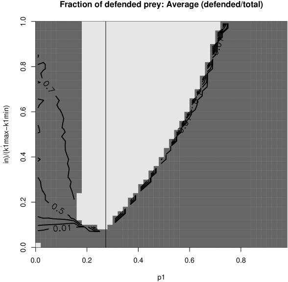
Figure 6: Contour plot of the long-term average fraction of defended prey. The horizontal axis is the palatability $p_{1}$ of the defended prey, with the model scaled so that $p_{2}=1$. The vertical axis represents $1/k_{1}$, with 0 and 1 corresponding to the lower and upper limits of the coexistence equilibrium region (Figure 4). Numerical solutions of the model were used to compute the long-term average value of $x_{1}/(x_{1}+x_{2})$ for parameter values such that the (predator + vulnerable prey) system (same parameter values as panel A of Fig. 5). In the lighter-gray region the coexistence equilibrium is stable. In the darker-gray region the equilibrium is unstable. The vertical black line is at $p_{1}=p^{*}$, the value where the straight and curved segments of the upper limit of the coexistence equilibrium region meet. Parameter values are as in Table 2 with $\delta=1.5$.

5.4 The structure of evolutionary cycles

The stability analysis above delimits the situations in which evolutionary cycles occur. As illustrated in Figure 5A, they arise when the $p_{1}$ versus $k_{1}$ tradeoff curve passes (with decreasing $p_{1}$) from the region of stable coexistence equilibria near $p_{1}=p^{*},k_{1}=k_{2}$ to the region of unstable coexistence equilibria with $p_{1}\approx 0$. For $1/k_{1}$ below the dash-dot curve in Figure 5A the defended prey cannot invade the vulnerable prey-predator limit cycle (see Figure 6). As $1/k_{1}$ increases, the defended prey becomes persistent and then increases in average abundance. As $1/k_{1}\to 1/k_{2}$ the characteristic features of evolutionary cycles emerge: longer cycle period and out-of-phase oscillations in predator and total prey abundance.

The phase relations on evolutionary cycles can be seen in the dominant eigenvector of the Jacobian matrix for the unstable fixed point (Figure 7). There is a codominant pair of complex conjugate eigenvalues, and ( because $\det(J)<0$ ) the third eigenvalue is real and negative. As the defended prey has very low palatability, the predator and the vulnerable prey have the classical quarter-phase lag. Here the phase angle is $90^{o}$; because eigenvectors are only defined up to arbitrary scalar multiples, including arbitrary rotations in the complex plane from multiplication by $e^{i\theta}$, only the relative phases of eigenvector components are meaningful. As $1/k_{1}$ increases, the eigenvector components for the two prey types become out of phase with each other ($\approx 180^{o}$ phase angle, right column of Figure 7). As a result, the predator and total prey densities are out of phase with each other.

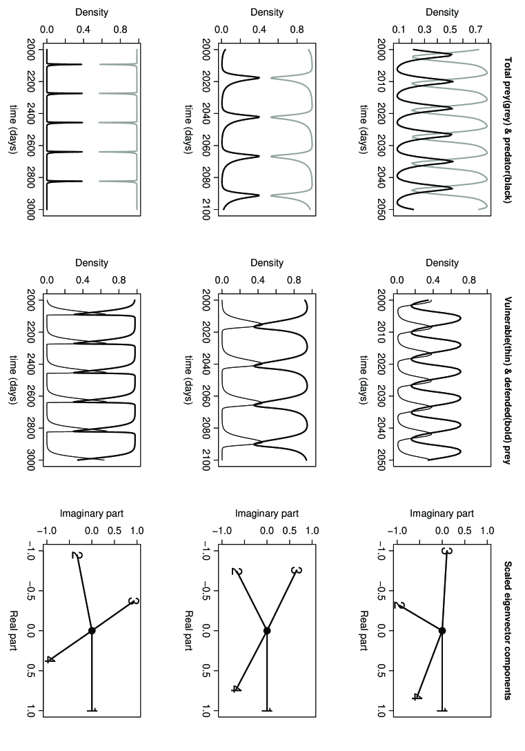
Figure 7: Coexistence of edible and defended prey on a limit cycle. Parameter values for all plots were $\delta=0.9,m=3.3/\delta,g=2.3/\delta,k_{2}=0.05,k_{b}=0.2,p_{2}=1,p_{1}=0.08$. Values of $k_{1}$ were 0.4 (top row), 0.1 (center row) and 0.055 (bottom row). In each row the leftmost panel shows the dynamics of total prey and predator densities, the center panel shows the dynamics of the two prey types, and the rightmost panel shows the phases of the Jacobian matrix components: 1=defended prey, 2=edible prey, 3=predator, 4=total prey.

In the next section we show that these phase relations become exact as the limit $k_{1}\to k_{2}$ is approached, for a general version of the model in which we do not specify the functional forms of the predator and prey functional responses.

6 Evolutionary cycles in a general two-prey model

In this section we analyze the limiting phase relations in evolutionary cycles, for $p_{1}\ll 1$ and low cost to defense, without specifying the functional forms of the prey and predator functional responses. We consider a two-prey, one-predator model that (after rescaling) can be written in the form

$$\begin{gathered}\dot{x}_{i}=x_{i}\left(f(X,y,\theta_{i})-p_{i}yg(Q)\right),i=1,2\hfill\\ \dot{y}=y\left(Qg(Q)-d\right)\hfill\\ \end{gathered}$$ (33)

where as usual $X=x_{1}+x_{2}$ is the total density of prey and $Q=p_{1}x_{1}+p_{2}x_{2}$ is the total prey quality as perceived by the predator. The key assumption in (LABEL:pmc) is total niche overlap in the prey types (e.g., because they are two clones within a single species), which is reflected in $f$ being a function of $X$. To model the trophic relations, $f$ is assumed to be strictly decreasing in $X$ and nonincreasing in $y$, and $h(Q)=Qg(Q)$ is strictly increasing in $Q$. Model (LABEL:pmc) includes the Abrams-Matsuda model [2] (a two-prey version of the Rosenzweig-MacArthur model with Lotka-Volterra competition between the prey) and the two-prey, one-predator chemostat model analyzed in the previous section of this paper.

The parameter $\theta_{i}$ in (LABEL:pmc) represents the prey-specific cost of defense, with $f$ decreasing in $\theta$. Because $f$ is decreasing in $X$, we can parameterize $f$ such that $\theta$ is the steady-state density for a single prey-type in the absence of predators, i.e.

$$f(\theta,0,\theta)=0.$$ (34)

As usual we number the prey so that $p_{1}<p_{2}$ and therefore $\theta_{1}<\theta_{2}$, and rescale the model so that $p_{2}=1$.

Evolutionary cycles can be viewed as arising when $\theta_{1}\uparrow\theta_{2}$ with $p_{1}\ll 1$, such that when $\theta_{1}\approx\theta_{2}$

1. There is a positive coexistence equilibrium with $\tilde{x}_{1},\tilde{x}_{2}$ converging to positive limits while $\tilde{y}\rightarrow 0$ as $\theta_{1}\uparrow\theta_{2}$;

2. The coexistence equilibrium is an unstable spiral for $\theta_{1}\approx\theta_{2}$.

At the end of this section, we show that Condition 1 always holds for (LABEL:pmc), and in Appendix F we show that the coexistence equilibrium is always a spiral. To determine the limiting phase relations, we need to find the eigenvector corresponding to the dominant eigenvalue with positive imaginary part (see Appendix A): the relative phase angles of this eigenvector’s components (in the complex plane) correspond to the phase lags between the corresponding state variables in solutions to the linearized system near the steady state.

The Jacobian for (LABEL:pmc) in the limit described above is

$$J_{0}=\left[{\begin{array}[]{*{20}c}\tilde{x}_{1}\tilde{f}_{X}&\tilde{x}_{1}\tilde{f}_{X}&\tilde{x}_{1}f_{y}-p_{1}\tilde{x}_{1}\tilde{g}\\ \tilde{x}_{2}\tilde{f}_{X}&\tilde{x}_{2}\tilde{f}_{X}&\tilde{x}_{2}f_{y}-\tilde{x}_{2}\tilde{g}\\ 0&0&0\\ \end{array}}\right].$$ (35)

The characteristic polynomial of (35) factors to show that the eigenvalues of (35) are $f_{X}(\tilde{x}_{1}+\tilde{x}_{2})<0$ and 0 as a repeated root; the first has corresponding eigenvector $(\tilde{x}_{1},\tilde{x}_{2},0)$, and for 0 there is the unique eigenvector $(1,-1,0)$. The zero eigenvalue therefore has algebraic multiplicity 2 and geometric multiplicity 1.

The long period of evolutionary cycles is explained by the fact that the dominant eigenvalues converge on a double-zero root as $\theta_{1}\to\theta_{2}$. The cycle period near the fixed point is inversely proportional to the imaginary part of the dominant eigenvalues, which converges to 0 in this limit.

To determine the limiting phase relations consider a small perturbation of the defended prey parameters, $\theta_{1}=\theta_{2}-\epsilon$. For $\epsilon$ small, we show in Appendix F that the double-zero eigenvalue is perturbed to a complex conjugate pair of eigenvalues. To study cycles, we assume that these have positive real part. That is, near the double-zero root the (scaled) characteristic polynomial is perturbed to leading order from $p(z)=z^{2}$ to $p(z)=(z-\epsilon a)^{2}+\epsilon b^{2}$ for some $b>0$, so the perturbed eigenvalues have $\textit{O}(\epsilon)$ real part and imaginary parts $\pm\sqrt{\epsilon}bi$ to leading order (here $i=\sqrt{-1}$). We need to determine the corresponding perturbed eigenvectors. Let $\vec{w_{0}}$ denote the unperturbed eigenvector $(1,-1,0)$, and let $\vec{w_{0}}+\vec{w_{e}}$ be a perturbed eigenvector corresponding to the complex eigenvalue with positive imaginary part, scaled so that its first component is 1. The first component of $\vec{w_{e}}$ is therefore 0. The perturbed Jacobian is $J_{0}+\epsilon J_{1}$ for some matrix $J_{1}$. Then

$$(J_{0}+\epsilon J_{1})(\vec{w_{0}}+\vec{w_{e}})=\sqrt{\epsilon}bi(\vec{w_{0}}+\vec{w_{e}})+\textit{O}(\epsilon).$$ (36)

Using $J_{0}\vec{w_{0}}=0$ and keeping only leading-order terms, gives

$$J_{0}\vec{w_{e}}=\sqrt{\epsilon}bi\vec{w_{0}}.$$ (37)

Let $\vec{w_{e}}=(0,w_{2},w_{3})$; then writing out (37) in full, $w_{2}$ and $w_{3}$ satisfy

$$\left[{\begin{array}[]{*{20}c}\tilde{x}_{1}f_{X}&\tilde{x}_{1}f_{y}-p_{1}\tilde{x}_{1}\tilde{g}\\ \tilde{x}_{2}f_{X}&\tilde{x}_{2}f_{y}-\tilde{x}_{2}\tilde{g}\\ \end{array}}\right]\left[{\begin{array}[]{*{20}c}w_{2}\\ w_{3}\\ \end{array}}\right]=\sqrt{\epsilon}bi\left[{\begin{array}[]{*{20}c}1\\ -1\\ \end{array}}\right].$$ (38)

$w_{2}$ and $w_{3}$ must be pure imaginary, because the unique solution to the real part of (38) is $(0,0)$. Writing $w_{j}=(\sqrt{\epsilon}bi)z_{j}$ and solving for the $z$’s, we find that $z_{2}<0$ and $z_{3}>0$; specifically

$$\left[{\begin{array}[]{*{20}c}z_{2}\\ z_{3}\\ \end{array}}\right]\propto\left[{\begin{array}[]{*{20}c}(\tilde{x}_{1}+\tilde{x}_{2})f_{y}-(p_{1}\tilde{x}_{1}+\tilde{x}_{2})\tilde{g}\\ -(\tilde{x}_{1}+\tilde{x}_{2})f_{X}\\ \end{array}}\right]=\begin{bmatrix}\tilde{X}f_{y}-d\\ -\tilde{X}f_{X}\\ \end{bmatrix}$$ (39)

using the fact that (from the second line of (LABEL:pmc))

$$\tilde{Q}g(\tilde{Q})=d.$$ (40)

So to leading order the eigenvector corresponding to eigenvalue $\sqrt{\epsilon}bi+o(\sqrt{\epsilon})$ is

$$\vec{w_{0}}+\vec{w_{e}}=\left[{\begin{array}[]{*{20}c}1\\ -1-\sqrt{\epsilon}Bi\\ \sqrt{\epsilon}Ci\\ \end{array}}\right]\mbox{ for some }B,C>0.$$ (41)

Now add total prey as a fourth state variable to the system. The corresponding eigenvector component is the sum of the first two components in (41) (see Appendix A):

$$\left[{\begin{array}[]{*{20}c}1\\ -1-\sqrt{\epsilon}Bi\\ \sqrt{\epsilon}Ci\\ -\sqrt{\epsilon}Bi\\ \end{array}}\right]$$ (42)

We can multiply each component of (41) by an arbitrary real constant without affecting the phase angles, so we can consider instead $\left(1,-1-\sqrt{\epsilon}Bi,i,-i\right).$ Then as $\epsilon\to 0$ the vector giving the relative phases for prey 1, prey 2, predator, and total prey becomes

$$\left[1\quad-1\quad i\quad-i\right]^{T}.$$ (43)

The components of the limiting phase-angle vector (43) lie exactly on the coordinate axes. The two prey types (first and second eigenvector components) are exactly out of phase; the predator and total prey (third and fourth components) are exactly out of phase; and there is a quarter-period lag between the vulnerable prey and the predator. This holds in the limit $\theta_{1}\to\theta_{2}$ for $p_{1}<p^{*}$ such that the coexistence equilibrium remains is an unstable spiral when $\theta_{1}<\theta_{2}$.

Finally, we now show that for $p_{1}$ sufficiently small there always exists coexistence equilibria as $\theta_{1}\uparrow\theta_{2}$ such that $\tilde{x}_{1},\tilde{x}_{2}$ approach finite limits while $\tilde{y}\to 0$. Evolutionary cycles then occur whenever these equilibria are unstable.

We must have $\theta_{2}>\tilde{Q}$ – this is just the condition that the vulnerable prey, at steady state, is a sufficient supply of food for the predator to increase when rare. Fix a value of $\tilde{y}>0$ – we will show that for any $\tilde{y}$ sufficiently small, there will be a value of $\theta_{1}\approx\theta_{2}$ such that there is a coexistence equilibrium with $\tilde{y}$ as the equilibrium prey density. A coexistence equilibrium must satisfy and the conditions

$$f(X,y,\theta_{i})=p_{i}yg(\tilde{Q}).$$ (44)

Let $\tilde{X}$ be defined as the solution of

$$f(\tilde{X},\tilde{y},\theta_{2})=\tilde{y}g(\tilde{Q}).$$

We have $f(\theta_{2},0,\theta_{2})=0$, so $\tilde{X}=\theta_{2}+O(\tilde{y})$. Then condition (44) for prey type 1 can be satisfied by choosing $\theta_{1}=\theta_{2}+O(\tilde{y})$ such that

$$f(\tilde{X},\tilde{y},\theta_{1})=p_{1}yg(\tilde{Q})$$

.

The last thing needing to be shown is that there exist $\tilde{x}_{1}>0,\tilde{x}_{2}>0$ such that

$$\tilde{x}_{1}+\tilde{x}_{2}=\tilde{X},\qquad p_{1}\tilde{x}_{1}+\tilde{x}_{2}=\tilde{Q}.$$

This is a system of two linear equations in the two unknowns $\tilde{x}_{1},\tilde{x}_{2}$ whose solution (by inverting a $2\times 2$ matrix) is

$$\left[{\begin{array}[]{*{20}c}{\tilde{x}_{1}}\\ {\tilde{x}_{2}}\\ \end{array}}\right]=\frac{1}{{1-p_{1}}}\left[{\begin{array}[]{*{20}c}{\tilde{X}-\tilde{Q}}\\ {\tilde{Q}-p_{1}\tilde{X}}\\ \end{array}}\right].$$ (45)

For $\tilde{y}$ small, $\tilde{X}\approx\theta_{2}>\tilde{Q}$ so $\tilde{x}_{1}>0$ in (45). And for $p_{1}$ sufficiently small, $p_{1}\tilde{X}<\tilde{Q}$ so $\tilde{x}_{2}>0$. So there do exist positive prey steady-states giving a coexistence equlibrium for $\tilde{y}$ near 0, and their limiting value (as $\tilde{y}\to 0$ and the corresponding $\theta_{1}\to\theta_{2}$) is given by (45) with $\tilde{X}=\theta_{2}$.

The argument above also identifies when $p_{1}$ is “sufficiently small” for the limiting values of $\tilde{x}_{1},\tilde{x}_{2}$ to be positive as $\theta_{1}\to\theta_{2}$. The limiting value of $\tilde{x}_{1}$ is always positive, and the limiting value of $\tilde{x}_{2}$ is positive if $p_{1}\tilde{X}-\tilde{Q}>0$ in the limit, i.e. if $p_{1}\theta_{2}<\tilde{Q}$. Thus, the coexistence equilibrium region extends up to the line $\theta_{1}=\theta_{2}$ so long as $p_{1}<p^{*}=\tilde{Q}/\theta_{2}.$

7 Discussion

The model studied in this paper is three dimensional, with a few fairly tame nonlinearities – just like the Lorenz equations. So it is not surprising that a complete mathematical analysis of the model has not been possible. Nonetheless, we have come a long way towards our goal of characterizing how and when rapid evolution can affect the ecological dynamics resulting from predator-prey interactions.

Our primary questions concern the generality of the phenomenon of “evolutionary” limit cycles in predator-prey interactions, and the conditions in which such cycles might be observed. A combination of analysis and numerical studies suggests that evolutionary dynamics are not omnipresent, but neither are they knife-edge phenomena existing only in a narrow range of parameter values. Instead, the types of cycles observed by Yoshida et al. [41, 43] are both robust and general. They occur in a specific but substantial and biologically relevant region of the parameter space, and in a general class of predator-two prey models that includes a two-prey model with Lotka-Volterra prey competition terms [2, 3, 25], and the standard two prey chemostat model [11, 23, 41] with mechanistic modeling of resource competition between the prey.

We have shown that evolutionary cycles arise through a bifurcation from a stable coexistence equilibrium, that occurs when defense against predation for the defended type remains relatively inexpensive but nevertheless becomes very effective. Cryptic population dynamics, where the predator cycles but the total prey density remains nearly constant, occur as a limiting case when effective defense comes at almost zero cost [43]. These regions in parameter space are biologically relevant because empirical studies have shown that defense - be it against predation or against antimicrobial compounds - can arise quickly and can be both highly effective and very cheap [4, 16, 42]. For example, Gagneux et al. [16] showed that in laboratory cultures of Mycobacterium tuberculosis (TB) mutants, prolonged treatment with antibiotics results in multi-drug resistant strains of TB with no fitness costs for resistance, and furthermore that most naturally circulating resistant TB strains are either low or no cost types. Indeed, fitness tradeoffs in the production of defensive structures and compounds are notoriously difficult to demonstrate, and in many empirical studies, no fitness tradeoff was actually found [4, 9, 37].

We close by listing some open questions. “Proving things is hard” (Hal Smith, personal communication), but others may succeed where we have not. Concerning the model in this paper,

• When does the Jacobian at a coexistence equilibrium have a pair of complex conjugate eigenvalues? There will be 3 real, negative eigenvalues if the two prey types are very similar and the interior equilibrium for the (predator + vulnerable prey) exists and is a stable node. However, our numerical results suggest the full system (at a coexistence equilibrium) has complex conjugate eigenvalues whenever the (predator+vulnerable prey) system has an interior equilibrium with complex conjugate eigenvalues.

• Can there be coexistence of the predator and both prey on a limit cycle or other attractor, even when there is no coexistence equilibrium? Numerical evidence suggests that the answer is “no” for the chemostat model: for $k_{1}$ below (above) the range of values at which a coexistence equilibrium exists, the defended (vulnerable) prey type outcompetes the other. As it is difficult to distinguish between persistence and slow competitive exclusion numerically, it is likewise hard to map reliably the parameter region where both prey coexist on a nonpoint attractor.

• On the bifurcation curve $0\leq p_{1}\leq p^{*},\quad k_{1}=k_{2}$, the Jacobian of the general model (LABEL:pmc) has zero as a double root with algebraic multiplicity 2 and geometric multiplicity 1. Generically, this situation gives a Takens-Bogdanov bifurcation [26]. Do the higher order conditions for Takens-Bogdanov, which hold generically, hold for our model (1)?

• A general two-prey, one-predator chemostat can exhibit a wider range of dynamic behaviors than we have observed in a system where the prey differ only in their $p$ and $k$ values (see [40] and references therein). Indeed, these predicted dynamics have been observed in other experimental systems [8]. The absence of some dynamics from our system, if true and verifiable, could indicate a qualitative difference between within-species evolutionary dynamics resulting from prey genetic diversity, and food-web dynamics with one predator feeding on a several prey species whose within-species heritable variation is much smaller than the functional differences among prey species.

Finally, how robust are the phenomena of evolutionary and cryptic predator-prey cycles in more complex food webs involving multiple predator and prey species?

Appendices

Appendices A and B summarize some general results useful to us here, and contain nothing original. In Appendix C we derive the expressions for coexistence steady states in the reduced and rescaled two-prey chemostat model, and in Appendix D we derive the Jacobian matrix and prove that it has negative determinant at any coexistence steady state. In Appendix E we derive the conditions in which a limit cycle of the (predator + edible prey) subsystem can can be invaded by the defended prey. Finally, in Appendix F we show generally that for realized cost $\theta_{1}$ sufficiently close to $\theta_{2}$ and $0\leq p_{1}\leq p^{*}$, the coexistence equilibrium for the general model (LABEL:pmc) always has a pair of complex conjugate eigenvalues.

Appendix A Appendix: Eigenvectors and phase relations

The contents of this Appendix appear to be well-known, but we have not seen them summarized anywhere in print. We consider oscillations in a linear system

$$\dot{x}=\mathbf{J}x$$ (46)

resulting from the real matrix $\mathbf{J}$ having complex conjugate eigenvalues

$$\lambda,\bar{\lambda}=a\pm ib\mbox{ with }b>0,$$

where $i=\sqrt{-1}$ and the overbar denotes complex conjugation. The corresponding eigenvectors are also a complex conjugate pair $w,\bar{w}$. The resulting oscillatory terms in solutions of (46) are of the general form $Ae^{\lambda t}w+Be^{\bar{\lambda}t}\bar{w}.$ In order for these to be real (as solutions of (46) must be), we must have $B=\bar{A}$. Then writing $A=re^{i\theta},r>0$, the solutions are proportional to

$$z(t)\equiv e^{i\theta}e^{ibt}w+e^{-i\theta}e^{-ibt}\bar{w}.$$ (47)

We are interested in the relative phases of the oscillations by different components in $z(t)$. Write $w_{j}=r_{j}e^{i\phi_{j}}$ for the $j^{th}$ component of $w$. The $j^{th}$ component of $z(t)$ is then

$$r_{j}(e^{i(\phi_{j}+\theta+bt)}+e^{-i(\phi_{j}+\theta+bt)})=2r_{j}\cos(\phi_{j}+\theta+bt).$$ (48)

The relative phases of the $j^{th}$ and $k^{th}$ components in solutions proportional to $z(t)$ is therefore given by $\phi_{j}-\phi_{k}.$ When this is near 0 components $j$ and $k$ are oscillating in phase, and when it is near $\pm\pi$ they are oscillating nearly out of phase.

We are interested in the phase difference between the predators and total prey density. For that we can use a linear change of variables

$$\left[{\begin{array}[]{*{20}c}u\\ v\\ y\\ \end{array}}\right]=\left[{\begin{array}[]{*{20}c}{x_{1}+x_{2}}\\ {x_{1}-x_{2}}\\ y\\ \end{array}}\right]=\mathbf{A}\left[{\begin{array}[]{*{20}c}{x_{1}}\\ {x_{2}}\\ y\\ \end{array}}\right],\quad\mathbf{A}=\left[{\begin{array}[]{*{20}c}1&1&0\\ 1&{-1}&0\\ 0&0&1\\ \end{array}}\right].$$

In transformed coordinates the Jacobian matrix becomes $\mathbf{AJA}^{-1}$, and Jacobian eigenvectors $w$ are transformed to $\mathbf{A}w$. The dominant eigenvector component for $x_{1}+x_{2}$ is therefore the sum of the components for $x_{1}$ and $x_{2}$.

Appendix B Appendix: Stability conditions

In this Appendix we review criteria for local stability of equilibria in a three-dimensional system of ordinary differential equations.

The diagonal expansion ([35], section 4.6) is an expression for $\det(A+D)$ where $A$ is square and $D$ is diagonal. For $D=xI$ and $A$ of order $n$ it states that

$$\det(A+xI)=x^{n}+x^{n-1}T_{1}(A)+x^{n-2}T_{2}(A)+\cdots+T_{n}(A)$$ (49)

where $T_{j}(A)$ is the sum of all principal minors of order $j$ (a principal minor of order $j$ is the determinant of a $j\times j$ submatrix of $A$ whose diagonal is a subset of the diagonal of $A$ – that is, a submatrix obtained by selecting $n-j$ diagonal elements of $A$ and deleting the row and column containing that element). Note that $T_{n}(A)=\det(A)$ and $T_{1}(A)=\mbox{trace}(A)$.

For a $3\times 3$ matrix the characteristic polynomial is

$$p(\lambda)\equiv\det(\lambda I-A)=\lambda^{3}+c_{2}\lambda^{2}+c_{1}\lambda+c_{0}.$$ (50)

Comparing with (49) and noting that and that $Tr_{j}(-A)=(-1)^{j}Tr_{j}(A)$, we have

$$c_{0}=T_{3}(-A)=-\det(A),\quad c_{1}=T_{2}(-A)=T_{2}(A),\quad c_{2}=\mbox{trace}(-A)=-\mbox{trace}(A).$$ (51)

In the notation of (50), the Routh-Hurwitz stability criteria for order-3 systems (May 1974) is

$$c_{0}>0,\quad c_{1}>0,\quad c_{2}>0,\quad c_{1}c_{2}>c_{0}.$$ (52)

Loss of stability through a Hopf bifurcation occurs when the third condition in (52) is violated, with the $c_{i}$ all positive [18].

Appendix C Coexistence steady states for the rescaled chemostat model

We consider here the two-prey model (10) Setting $\dot{y}=0$ and solving gives the steady state value of $Q$, $\tilde{Q}=\frac{k_{b}}{g-1}$. We solve for $\tilde{X}$ and $\tilde{y}$ as follows. Defining $Z=1-X-y$ and noting that $\frac{g}{k_{b}+\tilde{Q}}=\frac{1}{\tilde{Q}},$ the conditions $\dot{x}_{1}=\dot{x}_{2}=0$ imply

$$\frac{m\tilde{Z}}{k_{1}+\tilde{Z}}-\frac{p_{1}\tilde{y}}{\tilde{Q}}=\frac{m\tilde{Z}}{k_{2}+\tilde{Z}}-\frac{\tilde{y}}{\tilde{Q}}=1.$$ (53)

Solving (53) for $\tilde{y}$ gives two expressions which remain equal within the coexistence region:

$$\tilde{y}=\frac{\tilde{Q}}{p_{1}}\left[\frac{(m-1)\tilde{Z}-k_{1}}{k_{1}+\tilde{Z}}\right],\quad\tilde{y}=\tilde{Q}\left[\frac{(m-1)\tilde{Z}-k_{2}}{k_{2}+\tilde{Z}}\right].$$ (54)

Setting the two expressions for $\tilde{y}$ equal, we can solve for $\tilde{Z}$:

$$\tilde{Z}=\frac{1}{2(1-p_{1})(m-1)}\left[\zeta+\sqrt{\zeta^{2}+4(m-1)(1-p_{1})^{2}k_{1}k_{2}}\right]$$ (55)

where

$$\zeta=k_{1}\left(1+p_{1}(m-1)\right)-k_{2}\left((m-1)+p_{1}\right).$$

Finally, recalling that $\tilde{Z}=1-\tilde{X}-\tilde{y}$, then $\tilde{X}=1-\tilde{Z}-\tilde{y}.$ Expressions for $\tilde{x_{1}}$ and $\tilde{x_{2}}$ in terms of $\tilde{X}$ and $\tilde{Q}$ are derived and shown in the text.

Appendix D Jacobian at a coexistence equilibrium

The general expression (12) for Jacobian entries at a coexistence equilibrium implies that all entries in the $i^{th}$ row of the Jacobian have common factor $\tilde{x}_{i}$, so $\det(J)=\tilde{x}_{1}\tilde{x}_{2}\tilde{y}\det(\tilde{J})$ where $\tilde{J}(i,j)=\frac{\partial\tilde{r}_{i}}{\partial x_{j}}$ with $x_{3}=y$. Let $\tilde{F}$ denote the steady state per-capita feeding rate for the predator,

$$\tilde{F}=\frac{1}{k_{b}+p_{1}\tilde{x}_{1}+p_{2}\tilde{x}_{2}},$$ (56)

and the $a_{i}$ are defined by (31) with $\tilde{Z}=1-\tilde{x}_{1}-\tilde{x}_{2}-\tilde{y}$; equation (55) gives the general expression for $\tilde{Z}$.

Taking the necessary partial derivatives,

$$\tilde{J}=\left[{\begin{array}[]{*{20}c}{-a_{1}+gp_{1}^{2}\tilde{y}\tilde{F}^{2}}&{-a_{1}+gp_{1}p_{2}\tilde{y}\tilde{F}^{2}}&{-a_{1}-gp_{1}\tilde{F}}\\ {-a_{2}+gp_{1}p_{2}\tilde{y}\tilde{F}^{2}}&{-a_{2}+gp_{2}^{2}\tilde{y}\tilde{F}^{2}}&{-a_{2}-gp_{2}\tilde{F}}\\ {p_{1}gk_{b}\tilde{F}^{2}}&{p_{2}gk_{b}\tilde{F}^{2}}&0\\ \end{array}}\right].$$ (57)

We now show that the determinant of the Jacobian is always negative for the general model (LABEL:pmc), and therefore for the chemostat model, unless $p_{1}=p_{2}$. For (LABEL:pmc) with the scaling $p_{2}=1$ we have

$$\tilde{J}=\begin{bmatrix}f_{X}-p_{1}^{2}\tilde{y}\tilde{g}^{\prime}&f_{X}-p_{1}\tilde{y}\tilde{g}^{\prime}&f_{y}-p_{1}\tilde{g}\\ f_{X}-p_{1}\tilde{y}\tilde{g}^{\prime}&f_{X}-\tilde{y}\tilde{g}^{\prime}&f_{y}-\tilde{g}\\ \tilde{h}^{\prime}p&\tilde{h}^{\prime}&0\\ \end{bmatrix}$$ (58)

where $\tilde{g}=g(\tilde{Q}),\tilde{g}^{\prime}=g^{\prime}(\tilde{Q})$ and $\tilde{h}^{\prime}=h^{\prime}(\tilde{Q}),h(Q)=Qg(Q)$. Then using basic products of determinants, $\det(\tilde{J})$ equals

$$\tilde{h^{\prime}}\left|{\begin{array}[]{*{20}c}{f_{X}}&{f_{X}}&{f_{y}-p_{1}\tilde{g}}\\ {f_{X}}&{f_{X}}&{f_{y}-p_{1}\tilde{g}}\\ {p_{1}}&1&0\\ \end{array}}\right|=\tilde{h^{\prime}}\left|{\begin{array}[]{*{20}c}{f_{X}}&{f_{X}}&{f_{y}-p_{1}\tilde{g}}\\ 0&0&{(p_{1}-1)\tilde{g}}\\ {p_{1}}&1&0\\ \end{array}}\right|=(1-p_{1})^{2}\tilde{h^{\prime}}\tilde{g}f_{X}$$ (59)

which is negative (unless $p_{1}=1$) because $\tilde{h}^{\prime}>0,\tilde{g}>0$ and $f_{X}<0$.

Appendix E Appendix: Invasion of an edible prey limit cycle

Following [3] we give here the condition for invasion of a predator + edible prey limit cycle by a rare defended prey type. Along the limit cycle we have $\left\langle{\dot{\log}y}\right\rangle=0$ and therefore $\left\langle{\frac{gx_{2}}{k_{b}+x_{2}}}\right\rangle=1.$ By Jensen’s inequality, this implies that $\frac{g\left\langle{x_{2}}\right\rangle}{k_{b}+\left\langle{x_{2}}\right\rangle}>1$, and therefore $\left\langle{x_{2}}\right\rangle>\tilde{Q}$. We also have $\left\langle{\dot{\log x_{2}}}\right\rangle=0$ along the limit cycle, so

$$\left\langle{\frac{gy}{k_{b}+x_{2}}}\right\rangle=1+\left\langle{\frac{m(1-x_{2}-y)}{k_{2}+1-x_{2}-y}}\right\rangle.$$ (60)

A rare defended prey can invade if $\left\langle{\dot{\log x_{1}}}\right\rangle>0$, i.e. if

$$0<\left\langle{\frac{m(1-x_{2}-y)}{k_{1}+1-x_{2}-y}-p_{1}\frac{gy}{k_{b}+x_{2}}-1}\right\rangle=\left\langle{\frac{m(1-x_{2}-y)}{k_{1}+1-x_{2}-y}}\right\rangle-p_{1}\left\langle{\frac{gy}{k_{b}+x_{2}}}\right\rangle-1$$

Using (60) and simplifying, we get the invasion condition in terms of $p_{1},k_{1}$):

$$p_{1}<\frac{\left\langle{\zeta(k_{1})}\right\rangle-1}{\left\langle{\zeta(k_{2})}\right\rangle+1},$$ (61)

where

$$\zeta(k_{i})=\frac{m(1-x_{2}-y)}{k_{i}+1-x_{2}-y}.$$

Note that the right-hand side of (61) can be computed for all $k_{1}$ using one long simulation of the (predator + vulnerable prey) system, and yields $p_{1}$ as a function of $k_{1}$.

Appendix F Appendix: Eigenvalues for $\theta_{1}\uparrow\theta_{2},p_{1}\leq p^{*}$

We show here that for $\theta_{1}$ sufficiently close to $\theta_{2}$ and $0\leq p_{1}\leq p^{*}$ in the general model (LABEL:pmc), the coexistence equilibrium always has a pair of complex conjugate eigenvalues. As $\theta_{1}\to\theta_{2}$, in this range of $p_{1}$ values $\tilde{y}\to 0$, so we set $\tilde{y}=\epsilon\ll 1$ and use a series expansion in $\epsilon$ of the characteristic polynomial (i.e. we regard $\theta_{1}$ as a function of $\tilde{y}$ with all else held fixed, rather than vice versa). The Jacobian at the coexistence equilibrium is an $O(\epsilon)$ perturbation of (35) and so to leading order has the form

$$J(\epsilon)=\begin{bmatrix}A+\epsilon a_{11}&A+\epsilon a_{12}&B+\epsilon a_{13}\\ C+\epsilon a_{21}&C+\epsilon a_{22}&D+\epsilon a_{23}\\ \epsilon a_{31}&\epsilon a_{32}&0\\ \end{bmatrix}$$ (62)

with $A,B,C,D<0$, and $a_{31}=p_{1}a_{32}>0$ (the last holds because $\dot{y}/y$ is a function of $Q=p_{1}x_{1}+x_{2}$ with the scaling $p_{2}=1$). $J(0)$ has eigenvalues zero (with algebraic multiplicity 2) and $A+C<0$, and we need to approximate the near-zero eigenvalues for $\epsilon$ small. The characteristic polynomial of $J(\epsilon)$ is a cubic in $\lambda$ but the near-zero eigenvalues are at most $O(\sqrt{\epsilon})$, so for our purpose the $\lambda^{3}$ terms in the characteristic polynomial can be neglected. This leaves a quadratic polynomial in $\lambda$, which will have complex conjugate roots if its discriminant is negative. Using Maple to compute the characteristic polynomial of (62), discard $\lambda^{3}$ terms and expand the remainder about $\epsilon=0$, to leading order in $\epsilon$ the discriminant is

$$4\epsilon(a_{32}-a_{31})(A+C)(AD-BC)$$

which will be negative if $AD-BC>0$. Referring to (35) some algebra gives

$$AD-BC=\tilde{x}_{1}\tilde{x}_{2}\tilde{f}_{X}\tilde{g}(p_{1}-1)$$

which is positive because $f_{X}<0$, as desired.

References

• [1] Abrams P. A.: Effects of increased productivity on the abundances of trophic levels. American Naturalist (141) 351-371 (1993).
• [2] Abrams P. and H. Matsuda: Prey adaptation as a cause of predator-prey cycles. Evolution (51) 1742-1750 (1997).
• [3] Abrams, P.: Is predator-mediated coexistence possible in unstable systems? Ecology (80) 608-621 (1999).
• [4] Andersson D. I. and B. R. Levin: The biological cost of antibiotic resistance. Curr. Opin. Microbiol.(2) 489-493 (1999).
• [5] Antonovics J., A. D. Bradshaw and R. G. Turner: Heavy metal tolerance in plants. Advances Ecol. Res. (71) 1-85 (1971).
• [6] Ashley, M.V., M.F. Willson, O.R.W. Pergams, D.J. O’Dowd, S.M. Gende, and J.S. Brown.: Evolutionarily enlightened management. Biological Conservation (111) 115-123 (2003).
• [7] Barry M.: The costs of crest induction for Daphnia carinata. Oecologia (97) 278-288 (1994).
• [8] Becks L., F. M. Hilker, H. Malchow, K. Jürgens and H. Arndt: Experimental demonstration of chaos in a microbial foodweb. Nature (435) 1226-1229 (2005)
• [9] Bergelson J. and Purrington C. B.: Surveying patterns in the cost of resistance in plants. Am. Nat. (148) 536-558 (1996).
• [10] Bohannan B. J. M. and R. Lenski: Effect of prey heterogeneity on the response of a model food chain to resource enrichment. Am. Nat. (153) 73-82 (1999).
• [11] Butler G. J. and G. S. K. Wolkowicz: Predator-mediated competition in the chemostat. J. Math. Biol. (24) 167-191 (1986).
• [12] Coltman D. W., P. O’Donoghue, J. T. Jorgenson, J. T. Hogg, C. Strobeck and M. Festa-Blanchet: Undesirable evolutionary consequences of trophy-hunting. Nature (426)655-658 (2003).
• [13] Conover D. O. and S. B. Munch: Sustaining fisheries yields over evolutionary time scales. Science (297) 94-96 (2002).
• [14] Fussmann G. F., S. P. Ellner, K. W. Shertzer, and N. G. Hairston, Jr.: Crossing the Hopf bifurcation in a live predator-prey system. Science (290) 1358-1360 (2000).
• [15] Fussmann, G. F., S.P. Ellner, and N.G. Hairston, Jr.: Evolution as a critical component of plankton dynamics. Proc. Royal Society of London Series B (270) 1015-1022 (2003).
• [16] Gagneux S., C. D. Long, P. M. Small, T. Van, G. K. Schoolnik, and B. J. M. Bohannan. The competitive cost of antibiotic resistance in Mycobacterium tuberculosis. Science (312) 1944-1946 (2006).
• [17] Grant P. R. and B. R. Grant: Unpredictable evolution in a thirty year study of Darwin’s finches. Science (296) 707-710 (2002).
• [18] Guckenheimer J., M. Myers and B. Sturmfels: Computing Hopf Bifurcations I. SIAM J. Numer. Anal. (34) 1-27 (1997).
• [19] Hairston N. G. and W. E. Walton: Rapid evolution of a life-history trait. Proc. Natl. Acad. Sci. USA (83) 4831-4833 (1986).
• [20] Hairston N. G., S. P. Ellner, M. A. Geber, T. Yoshida and J. A. Fox: Rapid evolution and the convergence of ecological and evolutionary time. Ecology Letters (8) 1114-1127 (2005).
• [21] Heath D. D., J. W. Heath, C. A. Bryden, R. M. Johnson and C. W. Fox: Rapid evolution of egg size in captive salmon. Science. (299) 1738-1740 (2003).
• [22] Hendry A. P. and M. T. Kinnison: The pace of modern life: measuring rates of contemporary microevolution. Evolution (53) 1637-1653 (1999).
• [23] Jones, L.E. and S.P. Ellner: Evolutionary tradeoff and equilibrium in a predator-prey system. Bull. Math. Biol. (66) 1547-1573 (2004).
• [24] Kinnison M. T. and N. G. Hairston, Jr.: Eco-evolutionary conservation biology: contemporary evolution and the dynamics of persistence. Functional Ecology, submitted August 2006.
• [25] Kretzschmar M., R.M. Nisbet, and E. McCauley: A predator-prey model for zooplankton grazing on competing algal populations. Theor. Pop. Biol. (44) 32-66 (1993).
• [26] Kuznetsov Y. A.: Elements of applied bifurcation theory. Applied Mathematical Sciences 112, Chapter 8. Springer-Verlag, New York (1994).
• [27] Meyer J., S. P. Ellner, N.G. Hairston, Jr., L.E. Jones and T. Yoshida: Prey evolution of the time scale of predator–prey dynamics revealed by allele-specific quantitative PCR. Proc. Natl. Acad. Sci. (103) 10690-10695 (2006).
• [28] Olsen E. M., M. Heino, G. R. Lilly, M. J. Morgan, J. Brattey, and U. Dieckmann: Maturation trends indicative of rapid evolution preceded the collapse of northern cod. Nature. (428) 932-935 (2004).
• [29] Palumbi S.: The evolution explosion: how humans cause rapid evolutionary change. W. W. Norton, New York, NY (2001)
• [30] Pickett-Heaps, J. D.: Green Algae: Structure, Reproduction and Evolution in Selected Genera. Sinauer Associates, Sunderland MA (1975).
• [31] Preisser E. L., D. J. Bolnick, M. F. Benard: Scared to Death? The effects of intimidation and consumption in predator–prey interactions. Ecology (86) 501-509 (2005).
• [32] Reznick D.N., F. H. Shaw, F. H. Rodd, and R. G. Shaw: Evaluation of the rate of evolution in natural populations of guppies (Poecilia reticulata). Science (275) 1934-1937 (1997)
• [33] Saccheri, I. and I. Hanski: Natural selection and population dynamics. Trends in Ecology and Evolution 21, 341-347 (2006).
• [34] Shertzer K. W., S. P. Ellner, G. F. Fussmann, and N. G. Hairston, Jr.: Predator–prey cycles in an aquatic microcosm: testing hypotheses of mechanism. Journal of Animal Ecology (71) 802–815 (2002)
• [35] Searle S.R.: Matrix Algebra Useful for Statistics. John Wiley and Sons, New York (1982)
• [36] Smith H. L. and P. Waltman: The theory of the chemostat. Cambridge University Press (1995).
• [37] Strauss S. Y., J. A. Rudgers, J. A. Lau, and R. E. Irwin: Direct and ecological costs of resistance to herbivory. Trends Ecol. Evol. (17) 278-285 (2002).
• [38] Thompson J. N.: Rapid evolution as an ecological process. Trends Ecol. Evol. (13) 329-332 (1998).
• [39] Toth D. and M. Kot: Limit cycles in a chemostat model for a single species with age structure. Mathematical Biosciences 202, 194–217 (2006).
• [40] Vayenis, D.V. and S. Pavlou. Chaotic dynamics of a food web in a chemostat. Mathematical Biosciences 162, 69–84 (1999).
• [41] Yoshida T., L. E. Jones, S. P. Ellner, G. F. Fussmann, and N. G. Hairston, Jr.: Rapid evolution drives ecological dynamics in a predator-prey system. Nature(424) 303–306 (2003)
• [42] Yoshida T., S. P. Ellner and N. G. Hairston, Jr.: Evolutionary tradeoff between defense against grazing and competitive ability in a simple unicellular alga, Chlorella vulgaris. Proc. Roy. Soc. Lond. B. (271) 1947-1953 (2004).
• [43] Yoshida T., S. P. Ellner, L. E. Jones, and N. G. Hairston, Jr.: Cryptic population dynamics: rapid evolution masks trophic interaction. Submitted to PLOS Biology, September 2006.
• [44] Zimmer, C.: Rapid evolution can foil even the best-laid plans. Science (300) 895 (2003).