Network growth approach to macroevolution

Abstract

We propose a novel network growth model coupled with the competition interaction to simulate macroevolution. Our work shows that the competition plays an important role in macroevolution and it is more rational to describe the interaction between species by network structures. Our model presents a complete picture of the development of phyla and the splitting process. It is found that periodic mass extinction occurred in our networks without any extraterrestrial factors and the lifetime distribution of species is very close to fossil record. We also perturb networks with two scenarios of mass extinctions on different hierarchic levels in order to study their recovery.

1 INTRODUCTION

The ecosystem, which is formed from a myriad of interactions between various species, is one of the best-known examples of complexity. During the last decade, theoretical research on coevolution of species and the statistics of extinctions have been strongly influenced by the pioneering interdisciplinary work of Per Bak and his collaborators [1, 2, 3, 4]. Many simple and delicate models have been able to explain a large number of phenomena exhibited in the fossil record. Notably, with the development of nonlinear dynamics and complex network, it is found that food web model presents a most suitable way to describe ecosystem. More recent models based on network structure and various types of interaction have produced convincing results not only for macroevolution but also for microevolution. Microevolution that focuses on the influence of one species on others is more important in protecting the environment, whereas macroevolution, which focuses on species coevolution and periodic species extinction, is more interesting and important for species diversity.

Many remarkable phenomena have been found in the fossil record but, until now no satisfactory explanation has been presented. These phenomena include the Cambrian explosion that has given rise to all presently existing animal phyla, the periodicity of mass extinctions and characteristics of the evolution, such as extinction rate, origination rate, percent extinction, standing diversity, survivorship and lifetime distribution.

Recently, there have been attempts to study macroevolution using models equipped with dynamics that operate at the level of individuals [5, 6, 7]. Lotka-Volterra models are relatively successful in describing many aspects of population dynamics. Coppex has introduced a simple two-trophic network to describe an ecosystem with $N$ species of predators and one species of prey [8]. His numerical simulations show that there is a power-law distribution of intervals between extinctions. Since the Lotka-Volterra model is a differential equation model, it is hard to simulate the global-level processes with a large value of $N$. Furthermore, his model does not describe the macroevolution following the beginning of the Cambrian. Luz-Burgoa and cooperators have investigated the process of sympatric speciation in a simple food web model [9]. They find that sympatric speciation is obtained for the top species in both cases, and their results suggest that the speciation velocity depends on how far up, in the food chain, the focus population is feeding. In their later work a self-organized model without the need of two different resources has been presented [10]. However, these models investigate only the cause of species speciation and cannot explain the splitting process of a phylum.

B.F De Blasio and F.V. De Blasio have introduced competition interaction into the computer model of the influence of ecospace colonization on adaptive radiation designed by J. W. Valentine and T. D. Walker [11, 12]. This macroevolution model presents a clear picture of the simultaneous appearance of so many phyla in the Cambrian and the post-explosion evolution of the ecosystem. However, this model cannot show an accurate picture of macroevolution. It lacks periodicity of extinction and the results presented do not describe whether this model is consistent with the characteristics of the real fossil record. Moreover, this competition rule seems too simple to describe the intricate interaction between different species.

In fact, such interspecies competitive interactions play a key role in macroevolution whether considered as the sum of predator-prey interaction, host-parasite interaction or competitions between species using the same resource. Competition also appears to be essential for species proliferation. Laboratory bacterial experiments have suggested that species branching is promoted by competition [13, 14] and competition among higher taxonomical groups may also play a major role in macroevolution [15].

In this paper we present a macroevolution model also based on competitive interactions. In contrast to the model in Ref. [12], our model is built on the growth of network structures. From our simulation results of the properties, such as degree distribution, clustering coefficients, and especially the modularity dynamics, one can gain more insight into the processes of creating and splitting phyla and the possible effects of mass extinction. Additionally, we observe the periodicity of mass extinctions without any extraterrestrial causes (not mentioned in the model of Ref. [12]). This phenomenon is suggested by Raup and Sepkoski in $1984$ [16]. Our model indicates that this phenomenon, periodicity of mass extinctions, might be a natural consequence of macroevolution and not the result of any extraterrestrial causes as predicted by the model of Lipowski [17, 18]. Furthermore, the simulation results of lifetime distribution are very similar to the fossil record and the normal experiences of human beings. Finally, in order to study the effects of mass extinctions, large numbers of species were removed from network.

This article is organized as follows. We will explain how to build our model in Sec. 2. In Sec. 3, simulation results are shown and discussed, including network structure properties, lifetime distributions, extinction dynamics, and perturbations of the model. In the last Section, we summarize our conclusions and suggest some further extensions of our work.

2 NETWORK MODEL

We take every species as a point in 2-dimensional morphospace without boundary and let each dimension be independent. Each dimensional morphospace represents a phenotypic character of the species such as shape, form, structure, and so on. We select 2-dimensional morphospace as a compromise between integrated description of species and fast computation. Every species is characterized by a point in the morphospace. Species that belong to the same phylum are similar in phenotypic character, and they are close in morphospace. Phenotypic similarity between species implies that they are likely to exploit the same resources [19]. However, even species that are far from each other morphologically may compete for common resources, like the competition for light among plants and water among animals. Long-range competition is accounted for by allowing a finite tail in the possible competitive interaction for morphologically distant species. The model dynamics are subsequently described.

(1) Architecture of the network. Every node in the network represents one species and the weight of the connecting edge indicates the competition strength between two species. The evolution of the network represents the evolution of all species. We give the weight on the edges following a Gaussian-like form. It is chosen from the interval $[0,1]$, weighted as a truncated Gaussian of mean $0.5$ and the variance of the original, nontruncated Gaussian is also $0.5$. Once an edge is built, it does not change. However, when a species becomes extinct, we remove this node and all the edges connected to it from the network.

(2) Initialization. At the beginning, three species with the same phenotype are connected as the initial network. Then we assign the weights of three edges.

(3) Competition. Since not all species compete with each other even if they are very close in morphospace, the network model should not be a fully interconnected graph. The competition strength is equal to the weight of the edges. The extinction probability per step $p_{ext}$ of species $s_{i}$ depends on the total weight of edges connected with it. So the extinction probability of one species is defined by,

$$p_{ext}(s_{i})=\varepsilon\sum_{j}g_{ij},$$ (1)

where the $g_{ij}$ is the weight of the edge between species $s_{i}$ and $s_{j}$, and the fraction of competition $\varepsilon$ is constant. If one species becomes extinct, it will be erased from the network immediately and other species will no longer experience competition from the extinct one. As the network develops, the degree of the nodes increase and they will also feel more competition. The larger $p_{ext}$, the more easily species $s_{i}$ becomes extinct. Therefore, the $p_{ext}$ is hardly close to 1. If the $p_{ext}(s_{i})$ is larger than 1, we remove this species from the system.

(4) Speciation. In the short range, it appears to be approximately correct to say that the whole world can support a certain number of species. Modern-day ecological data on island biogeography support this view [20]. It is reasonable to assume that new species are more difficult to evolve as the species number approaches to this upper limit which is higher than that when the species is rare. When a new species originates from an old species, the distance in the morphospace between this new species and its parent for each dimension is Gaussian-distributed with mean $0$ and the standard deviation $\sigma$. Here, the $\sigma=0.1$ is the same for all simulations. New species is formed at each time step with the speciation rate,

$$p_{sp}=\beta\left(1-\frac{N}{N^{\prime}}\right),$$ (2)

where $\beta$ is the fraction of the speciation rate, $N^{\prime}$ is the maximal species number in the world, and $N$ is the current species number or node number in the network. In this work, the maximal species is set to $N^{\prime}=5500$ for all simulations.

After a new species was born, it becomes a part of the network, but it is isolated from other nodes. The probability $f(d_{ij})$ that the new node $i$ will be connected to the existent node $j$ ($j=i$ is excluded) depends on the distance between them in the morphospace.

$$f(d_{ij})=\left\{\begin{array}[]{ll}f_{0},&d_{ij}<R;\\ f_{\infty},&d_{ij}\geqslant R.\end{array}\right.$$ (3)

Here the $d_{ij}$ is the distance between species $s_{i}$ and $s_{j}$. We set the radius of short-range competition $R=2$ for all simulations, which was chosen larger than the speciation range $\sigma$ so that speciation takes place within the range of the short-range competition. The short-range competition factor $f_{0}$ should be much larger than the long-range competition factor $f_{\infty}$.

In this model, the reason for the survival of species alive is not its intrinsic morphological advantages but the morphological disparity of a species. In other words, the fitness landscape is flat. In each time step, we chose one species randomly and decided whether it would evolve into a new species based on the speciation rate. Then, we randomly selected another species and decided whether it should be removed from the network at that time step. This procedure is repeated millions of times in our simulations.

3 SIMULATION RESULT AND DISCUSSION

In this section we present the simulation results of our network model, such as degree distribution, clustering coefficient and community structure. Moreover, to study macroevolution we take the lifetime distribution, the extinction dynamics, and perturbation of network growth into account in our simulations .

3.1 Time Evolution of Network Structure

Figure 1: Temporal evolution of the structural properties of the network with parameters $\beta=0.6$, $\varepsilon=0.015$, $f_{0}=0.9$, and $f_{\infty}=0.03$. The insets show the magnification of the first $40000$ steps. A step-like increase is observed in the inset picture and corresponds to the split of the phyla.

Figure 2: Species distribution in morphospace at four different times. Top left, $10,000$ time steps after the beginning of simulation; top right, after $20,000$ time steps; bottom left, after $100,000$ time steps; bottom right, after $1,000,000$ time steps. The figure shows the dynamics of phylum split and the phylum branching process in morphospace. (More details about the splitting process can be seen at supplemental materials: http://www.youtube.com/watch?v=iJllf_tiaw0 and http://www.youtube.com/watch?v=87qqmMM1Dqc) The parameters of simulation are identical to those in Fig. 1.

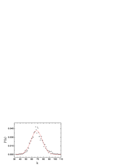
Figure 3: (Color online) Degree distribution of our network model with saturation node number $N\approx 2600$ after adequate steps simulation. Parameter values are $\beta=1.0$, $\varepsilon=0.015$, $f_{0}=0.5$, and $f_{\infty}=0.01$. The red line is a Gaussian fitting result with the mean $68.29184$ and variance $9.61$.

In general, two statistical properties, degree distribution and clustering coefficient, are used to measure the structures of complex networks. Clustering represents a common property of social network. Social network contains circles of friends or acquaintances in which every member knows each other. This tendency is quantified by the clustering coefficient. In our model, we use it to present the circles of competition existing between three species. For every node $i$ in the network, we could get $C_{i}=\frac{E_{i}}{k_{i}(k_{i}-1)/2}$, where $k_{i}$ is the degree of it and $E_{i}$ is the number of edges that existed between node $i$’s $k_{i}$ neighborhoods. The clustering coefficient of the whole network is the average of all individual $C_{i}$.

To study phylum splitting, we calculate the community structure of networks. Community structure is a mesoscopic description of networks. Newman and Girvan [21, 22] refers to the fact that nodes in many real networks appear to group in subgraphs. Like this property in the real networks, all the species can also be divided into different phyla. Therefore, the concept of community is used in our model to observe the phylum splitting. In our model, there is only one taxonomic group, so the community can be interpreted as genera, families, orders, classes, or any other taxonomic group. The strength of the community structure can be quantified by the modularity $Q$. Theoretically, the concept of modularity $Q$ cannot be used in weighted networks. Even then, community structure is still observed in the structural evolution in our simulations. The main reason for this observation is that in our model the connections among the nodes play a major role in the interspecies competition. Therefore we focus our attention on the structures and ignore the differences between the edges. In addition, we used the algorithm to find the community, as in Ref. [23], which is based on an extremal optimization of the value of modularity and is feasible for the accurate identification of community structure in large complex networks.

It should be noted that our model is a network with dynamic node number. Macroevolution is described by the process of network growth. In Fig. 1, we present how the species number, modularity and clustering coefficient evolve in the simulation. The main character of our simulation is that the network gradually stabilizes after an initial period of strong diversification. The inserted figure shows that the increasing species number and decreasing modularity and clustering coefficient are stepwise at the early phase. It should be noted that in the inserted figure the discrete transitions for species number, clustering coefficient, and modularity occur at the same time. These transitions denote the phylum splitting. When the model is on the plateau stage, the system is in a temporary stable state. The balance exists between the competition and the speciation rate. The process of phylum splitting is interesting. When the species get together to form a stable phylum, the diameter of every phylum on morphospace is about $R$ and the species in the phylum interact with short-range competition. Because there is a small distance between a new species and its parents, only the species on the fringe of the phylum contribute to the diffusion. The diameter of the phylum in morphospace increases. As the diameter of the phylum is larger than $R$, the central species of one phylum which is under strong competition from the fringe species are easily to extinct. The shrinking of central species facilitates the diffusion of fringe species. Diffusion and shrinking are not asymmetrical. Therefore, one phylum splits from the center and two parts separate gradually to form new phyla. Because the distance between two new phyla is larger than $R$, species will meet with more long-range competition from another phylum. The average number of species in the phylum will be smaller than that before splitting. Then the more phyla, the fewer species in every phylum. After the rapid increase in the initial phase, species proliferation decelerates to a constant value with little fluctuation. The modularity and clustering coefficient also decrease gradually while the species number increases slowly. This suggests that the number of community is increasing. This process can also be observed in Fig. 2.

The beginning increase of stepwise modularity can be interpreted by the definition given by Newman, $Q=\sum_{\gamma}(e_{\gamma\gamma}-a_{\gamma}^{2})$, where $e_{\gamma\gamma}$ is the fraction of edges that connect two nodes inside the community $\gamma$, $a_{\gamma}$ the fraction of links that have one or both nodes inside of the community $\gamma$. In our model, the definition can be written in the following form:

$$Q=\sum_{\gamma}\left(\frac{2z_{\gamma}^{in}}{2m}-\frac{2z_{\gamma}^{in}+z_{\gamma}^{ex}}{\left(2m\right)^{2}}\right),$$ (4)

where $m=\frac{1}{2}\sum_{\gamma}(2z_{\gamma}^{in}+z_{\gamma}^{ex})$ is the number of edges in the network, $z_{\gamma}^{in}$ is the number of edges which connect two nodes inside the community, and $z_{\gamma}^{ex}$ is the number of intercommunity edges. So only the network has many phyla and a large number of species in every phylum have the large $Q$. Considering that $f_{0}=0.9$ is much larger than $f_{\infty}=0.03$, we assume $z_{\gamma}^{in}\gg z_{\gamma}^{ex}$ and $z_{\gamma}^{in}=z_{\delta}^{in}$. We get

$$Q(n)\approx 1-1/n,$$ (5)

where $n$ is the community number in the network.

After the rapid increase in the initial phase, species proliferation decelerates to a constant value with little fluctuation. During this stage, the number of phyla is still increasing slowly. This phenomenon can be observed in Fig. 2(d). However, as discussed above, with increasing phyla in morphospace, the number of species in every phylum will decrease gradually. When the increase of $\gamma$ cannot compensate for the decrease of $z_{\gamma}^{in}$ and increase of $z_{\gamma}^{ex}$, the assumption $z_{\gamma}^{in}\gg z_{\gamma}^{ex}$ cannot be fulfilled anymore. Therefore modularity $Q$ will descend gradually. That is the reason for the decreasing modularity after the initial stage.

In Fig.  2, we present simulation results of the species distribution in morphospace at different times. Every point in the morphospace denotes a species. Obviously, species congregate around to form phylum. The figure on the bottom right is the species distribution of $1,000,000$ steps when the system has been on the stable stage and, once in stable stage, the number of phylum will not increase monotonously with the time, but every phylum’s position move slowly.

In order to understand the properties of the network model for biology, one must have some knowledge about the degree distribution $P(k)$, which is the probability that a node has degree $k$. Note that the number of vertices of this network model is dynamic. To study $P(k)$, it should be assigned large $\beta$ and other parameters as small to generate a network with a large number of nodes. In Fig. 3, we present the degree distribution of the network with $N\approx 2600$ at the final saturation state. It was found that P(k) is very close to a Gaussian distribution with mean $k\approx 68$. This distribution can be understood by a two-level random network. One is caused by the short-range competition, which has a few nodes in one community with connecting probability $f_{0}$. The other is caused by the long-range competition, which has many nodes whose number is almost equal to the whole nodes in the network with a connecting probability $f_{\infty}$. We know that in random networks, the modularity is very small and even close to 0. Therefore, it is difficult to categorize our network model as a type of network such as random, scale-free, or small-world.

3.2 Lifetime Distribution

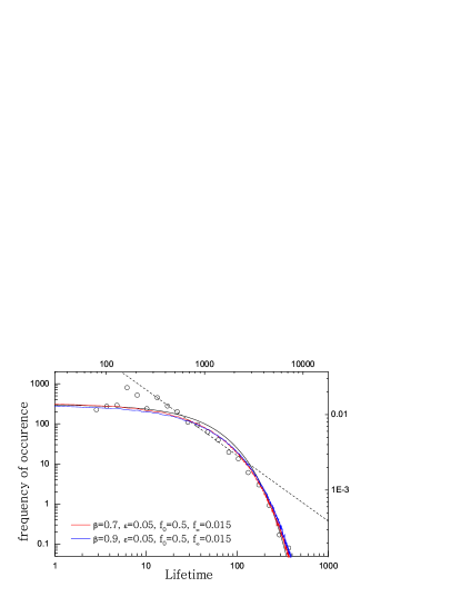
Figure 4: (Color online) Histogram of lifetimes of marine genera during the Phanerozoic (black circles). The black dash line is the best power-law fit to the points between 10 and 100 My and the black solid line is the best exponential fit to all the points  [24, 25]. The red and blue solid lines are our simulation results from the network growth model using two different parameters.

One of the properties frequently studied in macroevolution models is lifetime distribution of species. Newman and Sibani mathematically derived a number of relations between the normal quantities (extinction rates, diversity, lifetime distribution, etc.) and showed how these different trends are inter-related [25]. Since the lifetime distribution is easy to calculate, it becomes a canonical simulation result in most models of ecosystems.

Using simulations based on various models, many scholars have measured the lifetimes of competing species and suggested that their distribution is well approximated by a power-law form [25]. Similar estimations demonstrate that this distribution is equivalent to the power-law distribution of genus lifetimes, since the longer lived genera give rise on average to larger numbers of species [26]. However, the real fossil records are fit equally well by an exponential form [25].

In Fig. 4 we show a histogram of species lifetime distributions for the network growth model with two different parameters $\beta$. As the plot shows, the distribution closely follows an exponential law. Note that two simulation results of the lifetime distribution of species for different $\beta$ are very similar. We conjecture that the lifetime distribution of species is not under the influence of the fraction of the speciation rate $\beta$, but depends on the ratio between $f_{0}$ and $f_{\infty}$ (or the ratio between competition within a phylum and competition for resources). Moreover, this observation emphasizes that the competitive interactions play a key role in ecological dynamics.

3.3 Extinction Dynamics

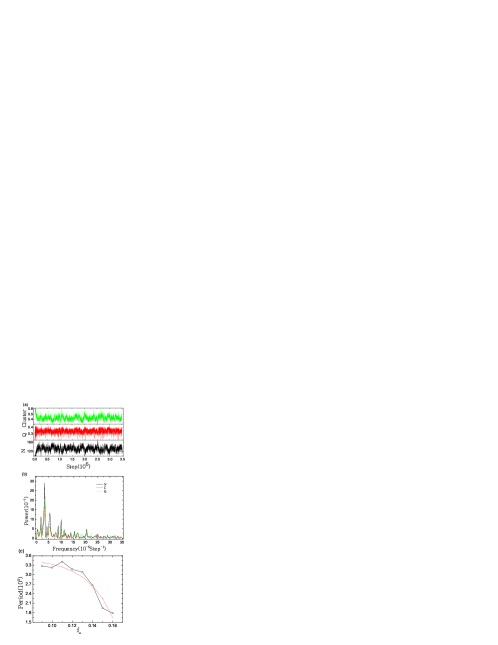
Figure 5: (Color online) Periodicity of mass extinctions without an extraterrestrial cause. Parameter values are $\beta=0.9$, $\varepsilon=0.05$, $f_{0}=0.9$, and $f_{\infty}=0.14$. (a) Time series of the clustering coefficient, modularity $Q$, and species number $N$. (b) The Power Spectral Density of the data in (a). (c) The maximal periodicity of oscillation $\tau$ from the time series of species number $N$ as a function of $f_{\infty}$. The other parameters are the same as in (a).

Of the estimated one to four billion species which have existed on the Earth since life first appeared here, less than 50 million are still alive today. Paleontological data, which show broad distributions of the extinct events in the Earth’s history, suggest the existence of strong correlations between extinctions [27]. Normally, the majority of researchers prefer the alternative explanation that the extinctions appear because of external stresses imposed on the ecosystems by the environment. Recently, the occurrence of extinctions in the absence of periodic external perturbation was suggested by Lipowski in a lattice model [17, 18].

Fig. 5 shows the temporal evolution of $N$, $Q$, and the clustering coefficient at the saturation state with parameters $\beta=0.9$, $\varepsilon=0.05$, $f_{0}=0.9$, and $f_{\infty}=0.14$. Note that we omit the initial phase of the network growth in Fig. 5(a). The Power Spectral Density of the data is presented in Fig. 5(b). In order to compare the periodicity of $N$, $Q$ and the clustering coefficient, we subtract their means and rescale these data to make them have the same amplitudes before the Fourier transform. The peak in Fig. 5(b) shows that the species number $N$ and the modularity $Q$ and the clustering coefficient of the network have the same periodicity and power spectral density. Three curves have the same peak at frequency $3.35693(\times 10^{-6}Step^{-1})$. The maximal periodicity of oscillations $\tau$ for various $f_{\infty}$ is shown in Fig. 5(c). The red dashed line is a fitted result $\tau=351410-375.074\mathtt{exp}(38.81\times f_{\infty})$. Therefore this oscillation indicates that the extinction is on the phylum level. The oscillation of the network structure parameters reflects the number and scale changing of phylum. Phylum which bears intense competition will decrease its scale or even this phylum will go extinct. In most instances, large numbers of phyla do not routinely go extinct, and they may belong to extant groups rather than constituting distinct phyla.

It should be noted that the species number in Fig. 5(a) is very small, $N\approx 140$, due to the larger long-range competition $f_{\infty}=0.14$. In fact, by enlarging the simulation results of the saturation phase in Fig. 1 with $f_{\infty}=0.03$, it was found that similar oscillation behaviors take place in the large networks. However, the oscillation in Fig. 1 appears to be small-amplitude fluctuations.

It is clear from Fig. 5(c) that the periodicity of oscillation is a function of $f_{\infty}$. Moreover, our extensive simulation results demonstrate that there is no obvious correlation between the periodicity and other parameters. When the system is in stable stage, there is a balance between the extinction rate and the speciation rate. The extinction rate is caused by the short-range competition coming from the species in the same phylum and long-range competition coming from the species in another phylum. The process of phylum splitting increases the species number and phylum number. Then the balance is disturbed. The species in the phylum will bear more competition from other phyla. Therefore the mass extinction happens. If $f_{\infty}=0$, new phylum would not be affected by other phyla. The mass extinction would be unconspicuous either. Therefore we conjecture that the long-range competition for public resources induces the oscillation of the species number. However, smaller $f_{\infty}$ or a scenario with abundant public resources would not only increase the system size $N$ and the phylum number, but also decrease the extinction of species and phyla. As a result, only a small fluctuation of species and phyla exists.

3.4 Perturbing the Model

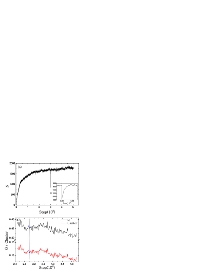
Figure 6: (Color online) The network growth with a random extinction at $3\times 10^{6}$ steps. (a) Time series of the species number. The inset shows a magnification of the extinction region. (b) The modularity and clustering coefficient in the extinction region. The dotted line is the time of extinction. The parameters are $\beta=0.5$, $\varepsilon=0.015$, $f_{0}=0.7$, and $f_{\infty}=0.015$ .

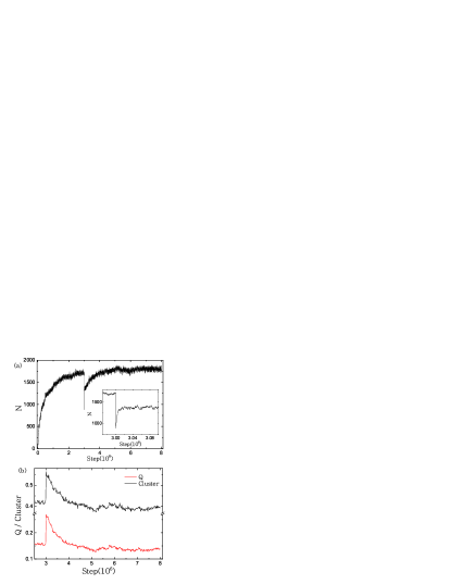
Figure 7: (Color online) The network growth with a random community extinction at $3\times 10^{6}$ steps. (a) The time evolution of the species number. The inset shows a magnification of the extinction region. (b) The modularity and cluster dynamics in the extinction region. The dotted line is the time of extinction. The parameters are identical to those used in Fig. 6.

In order to study the effect of mass extinctions on the macroevolution with the network growth approach, a large number of species were removed from the network at the saturation state. Such a scenario is designed to mimic the influence of an external factor, such as the change of climate, the impacts of comets or meteorites, etc. We discuss the following two cases.

Case I: Random perturbation on species. In this case, half of the species were removed randomly. Such a situation is appropriate for biosphere in which the species become extinct because of ’bad luck’. Clearly, the dynamics of the network should be reduced to the saturation state quickly since each species has the same probability of extinction.

Case II: Random perturbation on community. In this case, the artificial perturbations act on the community. We remove half of the community in the network randomly. The motivation for this case is based on the idea that some phyla have ’bad genes’ and cannot adapt to the sudden change of environment.

Figs. 6-7 show the simulation results of the time series of the species number and the network structure for both cases. Obviously, even though both scenarios of mass extinction act on different hierarchic levels, the species in the world will eventually recover and the response to an extinction will include a rapid expansion of species diversity. However, there is a noticeable difference, which can be seen in Fig. 6-7, in the detailed recovery process.

In case I, after removing nodes in the network, the species number quickly returned to the pre-perturbation level (see Fig. 6(a)). Fig. 6(b) depicts the response of network structure to extinction. There is not any significant change of the modularity and clustering coefficient and both are still in the normal fluctuation range.

In contrast to case I, the recovery in case II is slow and difficult. Many more steps are necessary for the species number to reach the saturation stage (see Fig. 7 (a)). However, note that there is also a sharply rising stage (as shown in the inset of Fig. 7(a)). The initial stage of the response to the extinction, when compared with the inset of Fig. 6(a), is similar for both cases. In Fig. 7(b), we present the responses of the modularity and clustering coefficient to this extinction. These curves represent a sudden increase preceding the decrease of the diversity at the phylum level.

As demonstrated by the arguments given above, it is clear that the response of the biological evolution for the two scenarios of mass extinction is completely different. Although both perturbations erase almost the same ratio of the species, in Case I the perturbation does not break down the structure of the network. In Case II, however, a number of whole communities are removed, or some phyla become extinct. Therefore the network structure is destroyed and the perturbation of Case II is more deleterious.

The statement above implies that forming phyla is a way for species to avoid or replace the short-range competition and increase the species number. Therefore it is much easier for species to conquer short-range competition for speciation than to develop long-range competition. In fact, in Case I, removing nodes in the network decreases both long- and short-range competition. The new species do not need to develop new phyla. This is the explaination of the fast recovery after disturbance. In contrast, Case II decreases the long-range competition. The new species develop in their phyla because the absence of long-range competition decreases the short-range competition below saturation and the small $\sigma$ make new species remain in their phyla. After this stage, when every phylum is full of species and reaches saturation, the new species develop new phyla. These new phyla are booming and force old phyla until they have the same scale. Thus, the behaviors of the modularity and cluster are different in two scenarios following disturbances, and the species number increases slowly to the saturation level after the initial sharply rising stage.

4 Conclusion

In this paper, we present a simple network growth model with competitive interactions to approximate the biological evolution. This model is characterized by four tunable parameters: the fraction of competition $\varepsilon$, the fraction of speciation rate $\beta$, the short-range competition $f_{0}$, and the long-range competition $f_{\infty}$. We start with a few species, and then let our model grow in diversity and complexity until it reaches the saturation state. It should be noted that the limitation $N^{\prime}$ plays an important role in the evolution. Without this parameter, periodical extinction cannot be displayed. These simulation results are not presented in this paper. Our model can be established on the higher dimensions, but it is difficult to show the community beyond the two-dimensional case. In a higher dimension case, a larger saturation species number on the stable state is formed. These results are not shown in this paper.

Based on the simulation results of our network growth model, we present several different aspects of biological evolution, such as the species number, phyla, clustering coefficient, and the lifetime distribution. We also observe the periodic mass extinction. Finally, the network model is perturbed in two different ways: random perturbation species and random perturbation on community. The effects of these different extinction scenarios on the two taxonomic hierarchic levels, species and phyla, may be useful to interpret of the causes of historical mass extinction.

Our model is aimed at emphasizing the importance of competition and network structure in the biological evolution. Competition not only decides the species number in the whole system, but also makes the species split to different phyla. As there are two kinds of different competitions, the responses of the biological evolution for two mass extinctions are completely different. Competition coupled with network structure drives the number of species to fluctuate periodically.

Although many of the properties shown in our model are similar to the fossil records especially the lifetime distribution, it is difficult to compare the model with the actual history of phyla diversities and real world. Since this model is a macroevolution model, it cannot include all the properties and details of biology.

Further extensions of our model offer interesting opportunities. For example, one can change the form of the competing function or differently implement the interaction among species. This could complicate the simulation tremendously, and we believe that the results would have the similar qualitative properties. In the real world, the climate switches between the ice age and warmth within a period of about $10,000$ years[28]. Comparably, our model could also use the periodic change parameters instead of the constant form. Such a modification would likely result in other thought-provoking phenomena. However, this modification is not currently reasonable because we cannot assess whether the changing climate is strong enough to affect the parameters in our model or whether a relationship exists between the climate and the model.

References

References

- [1] P. Bak and K. Sneppen, Phys. Rev. Lett. 71, 4083(1993); M. Paczuski, S. Maslov, and P. Bak, Phys. Rev. E 53, 414(1996).
- [2] R. V. Solé, S. C. Manrubia, M. Benton, and P. Bak, Nature 388, 764(1997).
- [3] P. Bak and S. Boettcher, Physica D 107, 143(1997).
- [4] R. V. Solé, S. C. Manrubia, M. Benton, S. Kauffman, and P. Bak, Trends in Ecology and Evolution, 14, 156(1999).
- [5] D. Chowdhury, D. Stauffer, and A. Kunwar, Phys. Rev. Lett. 90, 068101(2003).
- [6] P. A. Rikvold and R. K. P. Zia, Phys. Rev. E 68, 031913(2003).
- [7] M. Hall, K. Christensen, S. A. di Collobiano, and H. J. Jensen, Phys. Rev. E 66, 011904(2002).
- [8] F. Coppex, M. Droz, and A. Lipowski, Phys. Rev. E 69, 061901(2004).
- [9] K. Luz-Burgoa, T. Dell, and S. M. de Oliveira, Phys. Rev. E 72, 011914(2005).
- [10] K. Luz-Burgoa, S. Moss de Oliveira, Veit Schwmle, and J. S. S. Martins, Phys. Rev. E 74, 021910(2006).
- [11] J. W. Valentine, Paleobiology 6, 444(1980); J. W. Valentine and T. D. Walker, Physica D 22, 31(1986).
- [12] B. F. De Blasio and F. V. De Blasio, Phys. Rev. E 72, 031916(2005).
- [13] R. E. Lenski and M. Travisano, Proc. Natl. Acad. Sci. U.S.A. 91, 6808(1994).
- [14] D. Schluter, Science 266, 798(1994).
- [15] M. J. Benton, Biol. Rev. Cambridge Philos. Soc. 62, 305(1987); J. J. Sepkoski, in Paleobiology II: A Synthesis, edited by D.E. G. Briggs and P. R. Crowther (Blackwell Science, Malden, 2000).
- [16] D. M. Raup and J. J. Sepkoski, Proc. Natl. Acad. Sci. U.S.A. 81, 801(1984).
- [17] A. Lipowski, Phys. Rev. E 71, 052902(2005).
- [18] A. Lipowski and D. Lipowska, Theory. Biosci. 125, 67(2006).
- [19] A. R. H. Swan, in Paleobiology II: A Synthesis.
- [20] M. L. Rosenzweig Species Diversity in Space and Time. Cambridge University Press (Cambridge).(1995)
- [21] M. E. J. Newman and M. Girvan, Phys. Rev. E 69, 026113(2004).
- [22] M. Girvan and M. E. J. Newman, Proc. Natl. Acad. Sci. U.S.A. 99, 7821(2002).
- [23] J. Duch and A. Arenas, Phys. Rev. E 72, 027104(2005).
- [24] J. J. Jr Sepkoski, A compendium of fossil marine animal families, 2nd edition Milwaukee Public Museum Contributions in Biology and Geology 83, (1993).
- [25] M. E. J. Newman and P. Sibani, Proc. R. Soc. Lond. B 266, 1593(1999); B. Burlando, J. Theor, Biol. 146, 99(1990); M. E. J. Newman and K. Sneppen, Phys. Rev. E 54, 6226(1996).
- [26] C. Adami, Phys. Lett. A 203, 29(1995); K. Sneppen, P. Bak, H. Flyvbjerg, and M. H. Jensen, Proc. Natl. Acad. Sci. U.S.A. 92, 5209(1995); M. E. J. Newman, Physica D 107, 293(1997).
- [27] M. E. J. Newman and R. G. Palmer, Modelling Extinction (Oxford University Press, New York, 2003); M. E. J. Newman and R. G. Palmer, e-print adap-org/9908002.
- [28] P. M. Grootes and M. Stuiver, J. Geophys. Res. 102, 26455(1997).