Granger Causality: Basic Theory and Application to Neuroscience

Abstract

Multi-electrode neurophysiological recordings produce massive quantities of data. Multivariate time series analysis provides the basic framework for analyzing the patterns of neural interactions in these data. It has long been recognized that neural interactions are directional. Being able to assess the directionality of neuronal interactions is thus a highly desired capability for understanding the cooperative nature of neural computation. Research over the last few years has shown that Granger causality is a key technique to furnish this capability. The main goal of this article is to provide an expository introduction to the concept of Granger causality. Mathematical frameworks for both bivariate Granger causality and conditional Granger causality are developed in detail with particular emphasis on their spectral representations. The technique is demonstrated in numerical examples where the exact answers of causal influences are known. It is then applied to analyze multichannel local field potentials recorded from monkeys performing a visuomotor task. Our results are shown to be physiologically interpretable and yield new insights into the dynamical organization of large-scale oscillatory cortical networks.

1 Introduction

In neuroscience, as in many other fields of science and engineering, signals of interest are often collected in the form of multiple simultaneous time series. To evaluate the statistical interdependence among these signals, one calculates cross correlation functions in the time domain and ordinary coherence functions in the spectral domain. However, in many situations of interest, symmetric measures like ordinary coherence are not completely satisfactory, and further dissection of the interaction patterns among the recorded signals is required to parcel out effective functional connectivity in complex networks. Recent work has begun to consider the causal influence one neural time series can exert on another. The basic idea can be traced back to Wiener [1] who conceived the notion that, if the prediction of one time series could be improved by incorporating the knowledge of a second one, then the second series is said to have a causal influence on the first. Wiener’s idea lacks the machinery for practical implementation. Granger later formalized the prediction idea in the context of linear regression models [2]. Specifically, if the variance of the autoregressive prediction error of the first time series at the present time is reduced by inclusion of past measurements from the second time series, then the second time series is said to have a causal influence on the first one. The roles of the two time series can be reversed to address the question of causal influence in the opposite direction. From this definition it is clear that the flow of time plays a vital role in allowing inferences to be made about directional causal influences from time series data. The interaction discovered in this way may be reciprocal or it may be unidirectional.

Two additional developments of Granger’s causality idea are important. First, for three or more simultaneous time series, the causal relation between any two of the series may be direct, may be mediated by a third one, or may be a combination of both. This situation can be addressed by the technique of conditional Granger causality. Second, natural time series, including ones from economics and neurobiology, contain oscillatory aspects in specific frequency bands. It is thus desirable to have a spectral representation of causal influence. Major progress in this direction has been made by Geweke [3, 4] who found a novel time series decomposition technique that expresses the time domain Granger causality in terms of its frequency content. In this article we review the essential mathematical elements of Granger causality with special emphasis on its spectral decomposition. We then discuss practical issues concerning how to estimate such measures from time series data. Simulations are used to illustrate the theoretical concepts. Finally, we apply the technique to analyze the dynamics of a large-scale sensorimotor network in the cerebral cortex during cognitive performance. Our result demonstrates that, for a well designed experiment, a carefully executed causality analysis can reveal insights that are not possible with other techniques.

2 Bivariate Time Series and Pairwise Granger Causality

Our exposition in this and the next section follows closely that of Geweke [3, 4]. To avoid excessive mathematical complexity we develop the analysis framework for two time series. The framework can be generalized to two sets of time series [3].

2.1 Time Domain Formulation

Consider two stochastic processes $X_{t}$ and $Y_{t}$. Assume that they are jointly stationary. Individually, under fairly general conditions, each process admits an autoregressive representation

$$X_{t}=\sum^{\infty}_{j=1}a_{1j}X_{t-j}+\epsilon_{1t},\ \ \rm{var}(\epsilon_{1t})=\Sigma_{1}.$$ (1)

$$Y_{t}=\sum^{\infty}_{j=1}d_{1j}Y_{t-j}+\eta_{1t},\ \ \rm{var}(\eta_{1t})=\Gamma_{1}.$$ (2)

Jointly, they are represented as

$$X_{t}=\sum^{\infty}_{j=1}a_{2j}X_{t-j}+\sum^{\infty}_{j=1}b_{2j}Y_{t-j}+\epsilon_{2t},$$ (3)

$$Y_{t}=\sum^{\infty}_{j=1}c_{2j}X_{t-j}+\sum^{\infty}_{j=1}d_{2j}Y_{t-j}+\eta_{2t},$$ (4)

where the noise terms are uncorrelated over time and their contemporaneous covariance matrix is

$${\mathbf{\Sigma}}=\left(\begin{array}[]{cc}\Sigma_{2}&\Upsilon_{2}\\ \Upsilon_{2}&\Gamma_{2}\\ \end{array}\right).$$ (7)

The entries are defined as $\Sigma_{2}=\rm{var}(\epsilon_{2t}),\Gamma_{2}=\rm{var}(\eta_{2t}),\Upsilon_{2}=cov(\epsilon_{2t},\eta_{2t})$. If $X_{t}$ and $Y_{t}$ are independent, then $\{b_{2j}\}$ and $\{c_{2j}\}$ are uniformly zero, $\Upsilon_{2}=0$, $\Sigma_{1}=\Sigma_{2}$ and $\Gamma_{1}=\Gamma_{2}$. This observation motivates the definition of total interdependence between $X_{t}$ and $Y_{t}$ as

$$F_{X,Y}=\ln\frac{\Sigma_{1}\Gamma_{1}}{|{\mathbf{\Sigma}}|}$$ (8)

where $|\cdot|$ denotes the determinant of the enclosed matrix. According to this definition, $F_{X,Y}=0$ when the two time series are independent, and $F_{X,Y}>0$ when they are not.

Consider Eqs. (1) and (3). The value of $\Sigma_{1}$ measures the accuracy of the autoregressive prediction of $X_{t}$ based on its previous values, whereas the value of $\Sigma_{2}$ represents the accuracy of predicting the present value of $X_{t}$ based on the previous values of both $X_{t}$ and $Y_{t}$. According to Wiener [1] and Granger [2], if $\Sigma_{2}$ is less than $\Sigma_{1}$ in some suitable statistical sense, then $Y_{t}$ is said to have a causal influence on $X_{t}$. We quantify this causal influence by

$$F_{Y\rightarrow X}=\ln\frac{\Sigma_{1}}{\Sigma_{2}}.$$ (9)

It is clear that $F_{Y\rightarrow X}=0$ when there is no causal influence from $Y$ to $X$ and $F_{Y\rightarrow X}>0$ when there is. Similarly, one can define causal influence from $X$ to $Y$ as

$$F_{X\rightarrow Y}=\ln\frac{\Gamma_{1}}{\Gamma_{2}}.$$ (10)

It is possible that the interdependence between $X_{t}$ and $Y_{t}$ cannot be fully explained by their interactions. The remaining interdependence is captured by $\Upsilon_{2}$, the covariance between $\epsilon_{2t}$ and $\eta_{2t}$. This interdependence is referred to as instantaneous causality and is characterized by

$$F_{X\cdot Y}=\ln\frac{\Sigma_{2}\Gamma_{2}}{\left|\mathbf{\Sigma}\right|}.$$ (11)

When $\Upsilon_{2}$ is zero, $F_{X\cdot Y}$ is also zero. When $\Upsilon_{2}$ is not zero, $F_{X\cdot Y}>0$.

The above definitions imply that

$$F_{X,Y}=F_{X\rightarrow Y}+F_{Y\rightarrow X}+F_{X\cdot Y}.$$ (12)

Thus we decompose the total interdependence between two time series $X_{t}$ and $Y_{t}$ into three components: two directional causal influences due to their interaction patterns, and the instantaneous causality due to factors possibly exogenous to the $(X,Y)$ system (e.g. a common driving input).

2.2 Frequency Domain Formulation

To begin we define the lag operator $L$ to be $LX_{t}=X_{t-1}$. Rewrite Eqs. (3) and (4) in terms of the lag operator

$$\left(\begin{array}[]{cc}a_{2}(L)&b_{2}(L)\\ c_{2}(L)&d_{2}(L)\\ \end{array}\right)\left(\begin{array}[]{c}X_{t}\\ Y_{t}\\ \end{array}\right)=\left(\begin{array}[]{c}\epsilon_{2t}\\ \eta_{2t}\\ \end{array}\right),$$ (19)

where $a_{2}(0)=1,b_{2}(0)=0,c_{2}(0)=0,d_{2}(0)=1$. Fourier transforming both sides of Eq. (19) leads to

$$\left(\begin{array}[]{cc}a_{2}(\omega)&b_{2}(\omega)\\ c_{2}(\omega)&d_{2}(\omega)\\ \end{array}\right)\left(\begin{array}[]{c}X(\omega)\\ Y(\omega)\\ \end{array}\right)=\left(\begin{array}[]{c}E_{x}(\omega)\\ E_{y}(\omega)\\ \end{array}\right),$$ (26)

where the components of the coefficient matrix $\mathbf{A}(\omega)$ are

$$a_{2}(\omega)=1-\sum_{j=1}^{\infty}a_{2j}e^{-i\omega j},\ \ b_{2}(\omega)=-\sum_{j=1}^{\infty}b_{2j}e^{-i\omega j},$$

$$c_{2}(\omega)=-\sum_{j=1}^{\infty}c_{2j}e^{-i\omega j},\ \ d_{2}(\omega)=1-\sum_{j=1}^{\infty}d_{2j}e^{-i\omega j}.$$

Recasting Eq. (26) into the transfer function format we obtain

$$\left(\begin{array}[]{c}X(\omega)\\ Y(\omega)\\ \end{array}\right)=\left(\begin{array}[]{cc}H_{xx}(\omega)&H_{xy}(\omega)\\ H_{yx}(\omega)&H_{yy}(\omega)\\ \end{array}\right)\left(\begin{array}[]{c}E_{x}(\omega)\\ E_{y}(\omega)\\ \end{array}\right),$$ (33)

where the transfer function is $\mathbf{H}(\omega)=\mathbf{A}^{-1}(\omega)$ whose components are

$$H_{xx}(\omega)=\frac{1}{{\rm det}\mathbf{A}}d_{2}(\omega),\ \ H_{xy}(\omega)=-\frac{1}{{\rm det}\mathbf{A}}b_{2}(\omega),$$

$$H_{yx}(\omega)=-\frac{1}{{\rm det}\mathbf{A}}c_{2}(\omega),\ \ H_{yy}(\omega)=\frac{1}{{\rm det}\mathbf{A}}a_{2}(\omega).$$ (34)

After proper ensemble averaging we have the spectral matrix

$${\mathbf{S}}(\omega)={\mathbf{H}}(\omega){\mathbf{\Sigma}}{\mathbf{H}}^{*}(\omega)$$ (35)

where * denotes complex conjugate and matrix transpose.

The spectral matrix contains cross spectra and auto spectra. If $X_{t}$ and $Y_{t}$ are independent, then the cross spectra are zero and $|{\mathbf{S}}(\omega)|$ equals the product of two auto spectra. This observation motivates the spectral domain representation of total interdependence between $X_{t}$ and $Y_{t}$ as

$$f_{X,Y}(\omega)=\ln\frac{S_{xx}(\omega)S_{yy}(\omega)}{|\mathbf{S}(\omega)|},$$ (36)

where $|\mathbf{S}(\omega)|=S_{xx}(\omega)S_{yy}(\omega)-S_{xy}(\omega)S_{yx}(\omega)$ and $S_{yx}(\omega)=S_{xy}^{*}(\omega)$. It is easy to see that this decomposition of interdependence is related to coherence by the following relation:

$$f_{X,Y}(\omega)=-\ln(1-C(\omega)),$$ (37)

where coherence is defined as

$$C(\omega)=\displaystyle\frac{|S_{xy}(\omega)|^{2}}{S_{xx}(\omega)S_{yy}(\omega)}.$$

The coherence defined in this way is sometimes referred to as the squared coherence.

To obtain the frequency decomposition of the time domain causality defined in the previous section, we look at the auto spectrum of $X_{t}$:

$$S_{xx}(\omega)=H_{xx}(\omega)\Sigma_{2}H_{xx}^{*}(\omega)+2\Upsilon_{2}{\rm Re}(H_{xx}(\omega)H_{xy}^{*}(\omega))+H_{xy}(\omega)\Gamma_{2}H_{xy}^{*}(\omega).$$ (38)

It is instructive to consider the case where $\Upsilon_{2}=0$. In this case there is no instantaneous causality and the interdependence between $X_{t}$ and $Y_{t}$ is entirely due to their interactions through the regression terms on the right hand sides of Eqs. (3) and (4). The spectrum has two terms. The first term, viewed as the intrinsic part, involves only the variance of $\epsilon_{2t}$, which is the noise term that drives the $X_{t}$ time series. The second term, viewed as the causal part, involves only the variance of $\eta_{2t}$, which is the noise term that drives $Y_{t}$. This power decomposition into an “intrinsic” term and a “causal” term will become important for defining a measure for spectral domain causality.

When $\Upsilon_{2}$ is not zero it becomes harder to attribute the power of the $X_{t}$ series to different sources. Here we consider a transformation introduced by Geweke [3] that removes the cross term and makes the identification of an intrinsic power term and a causal power term possible. The procedure is called normalization and it consists of left-multiplying

$$\mathbf{P}=\left(\begin{array}[]{cc}1&0\\ -\displaystyle{\frac{\Upsilon_{2}}{\Sigma_{2}}}&1\\ \end{array}\right)$$ (39)

on both sides of Eq. (26). The result is

$$\left(\begin{array}[]{cc}a_{2}(\omega)&b_{2}(\omega)\\ c_{3}(\omega)&d_{3}(\omega)\\ \end{array}\right)\left(\begin{array}[]{c}X(\omega)\\ Y(\omega)\\ \end{array}\right)=\left(\begin{array}[]{c}E_{x}(\omega)\\ \tilde{E}_{y}(\omega)\\ \end{array}\right),$$ (46)

where $c_{3}(\omega)=c_{2}(\omega)-\displaystyle{\frac{\Upsilon_{2}}{\Sigma_{2}}}a_{2}(\omega),d_{3}(\omega)=d_{2}(\omega)-\displaystyle{\frac{\Upsilon_{2}}{\Sigma_{2}}}b_{2}(\omega),\tilde{E}_{y}(\omega)=E_{y}(\omega)-\displaystyle{\frac{\Upsilon_{2}}{\Sigma_{2}}}E_{x}(\omega)$. The new transfer function $\tilde{\mathbf{H}}(\omega)$ for (46) is the inverse of the new coefficient matrix $\tilde{\mathbf{A}}(\omega)$:

$$\tilde{\mathbf{H}}(\omega)=\left(\begin{array}[]{cc}\tilde{H}_{xx}(\omega)&\tilde{H}_{xy}(\omega)\\ \tilde{H}_{yx}(\omega)&\tilde{H}_{yy}(\omega)\\ \end{array}\right)=\frac{1}{\det\tilde{\mathbf{A}}}\left(\begin{array}[]{cc}d_{3}(\omega)&-b_{2}(\omega)\\ -c_{3}(\omega)&a_{2}(\omega)\\ \end{array}\right).$$ (47)

Since $\det\tilde{\mathbf{A}}=\det\mathbf{A}$ we have

$$\tilde{H}_{xx}(\omega)=H_{xx}(\omega)+\displaystyle{\frac{\Upsilon_{2}}{\Sigma_{2}}}H_{xy}(\omega),\ \ \tilde{H}_{xy}(\omega)=H_{xy}(\omega),$$

$$\tilde{H}_{yx}(\omega)=H_{yx}(\omega)+\displaystyle{\frac{\Upsilon_{2}}{\Sigma_{2}}}H_{xx}(\omega),\ \ \tilde{H}_{yy}(\omega)=H_{yy}(\omega).$$ (48)

From the construction it is easy to see that $E_{x}$ and $\tilde{E}_{y}$ are uncorrelated, that is, $\rm{cov}(E_{x},\tilde{E}_{y})=0$. The variance of the noise term for the normalized $Y_{t}$ equation is $\tilde{\Gamma}_{2}=\Gamma_{2}-\displaystyle{\frac{\Upsilon^{2}_{2}}{\Sigma_{2}}}$. From Eq. (46), following the same steps that lead to Eq. (38), the spectrum of $X_{t}$ is found to be:

$$S_{xx}(\omega)=\tilde{H}_{xx}(\omega)\Sigma_{2}\tilde{H}_{xx}^{*}(\omega)+H_{xy}(\omega)\tilde{\Gamma}_{2}H_{xy}^{*}(\omega).$$ (49)

Here the first term is interpreted as the intrinsic power and the second term as the causal power of $X_{t}$ due to $Y_{t}$. This is an important relation because it explicitly identifies that portion of the total power of $X_{t}$ at frequency $\omega$ that is contributed by $Y_{t}$. Based on this interpretation we define the causal influence from $Y_{t}$ to $X_{t}$ at frequency $\omega$ as

$$f_{Y\rightarrow X}(\omega)=\ln\frac{S_{xx}(\omega)}{\tilde{H}_{xx}(\omega)\Sigma_{2}\tilde{H}_{xx}^{*}(\omega)}.$$ (50)

Note that this definition of causal influence is expressed in terms of the intrinsic power rather than the causal power. It is expressed in this way so that the causal influence is zero when the causal power is zero (i.e., the intrinsic power equals the total power), and increases as the causal power increases (i.e., the intrinsic power decreases).

By taking the transformation matrix as $\left(\begin{array}[]{cc}1&-\Upsilon_{2}/\Gamma_{2}\\ 0&1\\ \end{array}\right)$ and performing the same analysis, we get the causal influence from $X_{t}$ to $Y_{t}$:

$$f_{X\rightarrow Y}(\omega)=\ln\frac{S_{yy}(\omega)}{\hat{H}_{yy}(\omega)\Gamma_{2}\hat{H}_{yy}^{*}(\omega)},$$ (51)

where $\hat{H}_{yy}(\omega)=H_{yy}(\omega)+\displaystyle{\frac{\Upsilon_{2}}{\Gamma_{2}}}H_{yx}(\omega)$.

By defining the spectral decomposition of instantaneous causality as [5]

$$f_{X\cdot Y}(\omega)=\ln\frac{(\tilde{H}_{xx}(\omega)\Sigma_{2}\tilde{H}_{xx}^{*}(\omega))(\hat{H}_{yy}(\omega)\Gamma_{2}\hat{H}_{yy}^{*}(\omega))}{|\mathbf{S}(\omega)|},$$ (52)

we achieve a spectral domain expression for the total interdependence that is analogous to Eq. (12) in the time domain, namely:

$$f_{X,Y}(\omega)=f_{X\rightarrow Y}(\omega)+f_{Y\rightarrow X}(\omega)+f_{X\cdot Y}(\omega).$$ (53)

We caution that the spectral instantaneous causality may become negative for some frequencies in certain situations and may not have a readily interpretable physical meaning.

It is important to note that, under general conditions, these spectral measures relate to the time domain measures as:

$$F_{Y,X} = \frac{1}{2\pi}\int_{-\pi}^{\pi}f_{Y,X}(\omega)d\omega,$$

$$F_{Y\rightarrow X} = \frac{1}{2\pi}\int_{-\pi}^{\pi}f_{Y\rightarrow X}(\omega)d\omega,$$

$$F_{X\rightarrow Y} = \frac{1}{2\pi}\int_{-\pi}^{\pi}f_{X\rightarrow Y}(\omega)d\omega,$$

$$F_{Y\cdot X} = \frac{1}{2\pi}\int_{-\pi}^{\pi}f_{Y\cdot X}(\omega)d\omega.$$ (54)

The existence of these equalities gives credence to the spectral decomposition procedures described above.

3 Trivariate Time Series and Conditional Granger Causality

For three or more time series one can perform a pairwise analysis and thus reduce the problem to a bivariate problem. This approach has some inherent limitations. For example, for the two coupling schemes in Figure 1, a pairwise analysis will give the same patterns of connectivity like that in Figure 1(b). Another example involves three processes where one process drives the other two with differential time delays. A pairwise analysis would indicate a causal influence from the process that receives an early input to the process that receives a late input. To disambiguate these situations requires additional measures. Here we define conditional Granger causality which has the ability to resolve whether the interaction between two time series is direct or is mediated by another recorded time series and whether the causal influence is simply due to differential time delays in their respective driving inputs. Our development is for three time series. The framework can be generalized to three sets of time series [4].

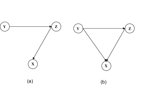
Figure 1: Two distinct patterns of connectivity among three time series. A pairwise causality analysis cannot distinguish these two patterns.

3.1 Time Domain Formulation

Consider three stochastic processes $X_{t}$, $Y_{t}$ and $Z_{t}$. Suppose that a pairwise analysis reveals a causal influence from $Y_{t}$ to $X_{t}$. To examine whether this influence has a direct component (Figure 1(b)) or is mediated entirely by $Z_{t}$ (Figure 1(a)) we carry out the following procedure. First, let the joint autoregressive representation of $X_{t}$ and $Z_{t}$ be

$$X_{t}=\sum^{\infty}_{j=1}a_{3j}X_{t-j}+\sum^{\infty}_{j=1}b_{3j}Z_{t-j}+\epsilon_{3t},$$ (55)

$$Z_{t}=\sum^{\infty}_{j=1}c_{3j}X_{t-j}+\sum^{\infty}_{j=1}d_{3j}Z_{t-j}+\gamma_{3t},$$ (56)

where the covariance matrix of the noise terms is

$${\mathbf{\Sigma}}_{3}=\left(\begin{array}[]{cc}\Sigma_{3}&\Upsilon_{3}\\ \Upsilon_{3}&\Gamma_{3}\\ \end{array}\right).$$ (59)

Next we consider the joint autoregressive representation of all three processes $X_{t}$, $Y_{t}$ and $Z_{t}$

$$X_{t}=\sum^{\infty}_{j=1}a_{4j}X_{t-j}+\sum^{\infty}_{j=1}b_{4j}Y_{t-j}+\sum^{\infty}_{j=1}c_{4j}Z_{t-j}+\epsilon_{4t},$$ (60)

$$Y_{t}=\sum^{\infty}_{j=1}d_{4j}X_{t-j}+\sum^{\infty}_{j=1}e_{4j}Y_{t-j}+\sum^{\infty}_{j=1}g_{4j}Z_{t-j}+\eta_{4t},$$ (61)

$$Z_{t}=\sum^{\infty}_{j=1}u_{4j}X_{t-j}+\sum^{\infty}_{j=1}v_{4j}Y_{t-j}+\sum^{\infty}_{j=1}w_{4j}Z_{t-j}+\gamma_{4t},$$ (62)

where the covariance matrix of the noise terms is

$$\mathbf{\Sigma}_{4}=\left(\begin{array}[]{ccc}\Sigma_{xx}&\Sigma_{xy}&\Sigma_{xz}\\ \Sigma_{yx}&\Sigma_{yy}&\Sigma_{yz}\\ \Sigma_{zx}&\Sigma_{zy}&\Sigma_{zz}\\ \end{array}\right).$$ (66)

From these two sets of equations we define the Granger causality from $Y_{t}$ to $X_{t}$ conditional on $Z_{t}$ to be

$$F_{Y\rightarrow X|Z}=\ln\frac{\Sigma_{3}}{\Sigma_{xx}}.$$ (67)

The intuitive meaning of this definition is quite clear. When the causal influence from $Y_{t}$ to $X_{t}$ is entirely mediated by $Z_{t}$ (Fig. 1(a)), $\{b_{4j}\}$ is uniformly zero, and $\Sigma_{xx}=\Sigma_{3}$. Thus, we have $F_{Y\rightarrow X|Z}=0$, meaning that no further improvement in the prediction of $X_{t}$ can be expected by including past measurements of $Y_{t}$. On the other hand, when there is still a direct component from $Y_{t}$ to $X_{t}$ (Fig. 1(b)), the inclusion of past measurements of $Y_{t}$ in addition to that of $X_{t}$ and $Z_{t}$ results in better predictions of $X_{t}$, leading to $\Sigma_{xx}<\Sigma_{3}$, and $F_{Y\rightarrow X|Z}>0$.

3.2 Frequency Domain Formulation

To derive the spectral decomposition of the time domain conditional Granger causality we carry out a normalization procedure like that for the bivariate case. For Eqs. (55) and (56) the normalized equations are

$$\left(\begin{array}[]{cc}D_{11}(L)&D_{12}(L)\\ D_{21}(L)&D_{22}(L)\\ \end{array}\right)\left(\begin{array}[]{c}x_{t}\\ z_{t}\\ \end{array}\right)=\left(\begin{array}[]{c}x_{t}^{*}\\ z_{t}^{*}\\ \end{array}\right),$$ (74)

where $D_{11}(0)=1,D_{22}(0)=1,D_{12}(0)=0$, $\mathrm{cov}(x^{*}_{t},z^{*}_{t})=0$, and $D_{21}(0)$ is generally not zero. We note that $\rm{var}(x_{t}^{*})=\Sigma_{3}$ and this becomes useful in what follows.

For Eqs. (60), (61) and (62) the normalization process involves left-multiplying both sides by the matrix

$$\mathbf{P}=\mathbf{P}_{2}\cdot\mathbf{P}_{1}$$

where

$$\mathbf{P}_{1}=\left(\begin{array}[]{ccc}1&0&0\\ -\Sigma_{yx}\Sigma_{xx}^{-1}&1&0\\ -\Sigma_{zx}\Sigma_{xx}^{-1}&0&1\\ \end{array}\right),$$ (78)

and

$$\mathbf{P}_{2}=\left(\begin{array}[]{ccc}1&0&0\\ 0&1&0\\ 0&-(\Sigma_{zy}-\Sigma_{zx}\Sigma_{xx}^{-1}\Sigma_{xy})(\Sigma_{yy}-\Sigma_{yx}\Sigma_{xx}^{-1}\Sigma_{xy})^{-1}&1\\ \end{array}\right).$$ (82)

We denote the normalized equations as

$$\left(\begin{array}[]{ccc}B_{11}(L)&B_{12}(L)&B_{13}(L)\\ B_{21}(L)&B_{22}(L)&B_{23}(L)\\ B_{31}(L)&B_{32}(L)&B_{33}(L)\\ \end{array}\right)\left(\begin{array}[]{c}x_{t}\\ y_{t}\\ z_{t}\\ \end{array}\right)=\left(\begin{array}[]{c}\epsilon_{xt}\\ \epsilon_{yt}\\ \epsilon_{zt}\\ \end{array}\right),$$ (92)

where the noise terms are independent, and their respective variances are $\hat{\Sigma}_{xx}$, $\hat{\Sigma}_{yy}$ and $\hat{\Sigma}_{zz}$.

To proceed further we need the following important relation [4]

$$F_{Y\rightarrow X|Z}=F_{YZ^{*}\rightarrow X^{*}}$$ (93)

and its frequency domain counterpart:

$$\textsl{f}_{Y\rightarrow X|Z}(\omega)=\textsl{f}_{YZ^{*}\rightarrow X^{*}}(\omega).$$ (94)

To obtain $\textsl{f}_{YZ^{*}\rightarrow X^{*}}(\omega)$, we need to decompose the spectrum of $X^{*}$. The Fourier transform of Eqs. (74) and (92) gives:

$$\left(\begin{array}[]{c}X(\omega)\\ Z(\omega)\\ \end{array}\right)=\left(\begin{array}[]{cc}G_{xx}(\omega)&G_{xz}(\omega)\\ G_{zx}(\omega)&G_{zz}(\omega)\\ \end{array}\right)\left(\begin{array}[]{c}X^{*}(\omega)\\ Z^{*}(\omega)\\ \end{array}\right),$$ (101)

and

$$\left(\begin{array}[]{c}X(\omega)\\ Y(\omega)\\ Z(\omega)\\ \end{array}\right)=\left(\begin{array}[]{ccc}H_{xx}(\omega)&H_{xy}(\omega)&H_{xz}(\omega)\\ H_{yx}(\omega)&H_{yy}(\omega)&H_{yz}(\omega)\\ H_{zx}(\omega)&H_{zy}(\omega)&H_{zz}(\omega)\\ \end{array}\right)\left(\begin{array}[]{c}E_{x}(\omega)\\ E_{y}(\omega)\\ E_{z}(\omega)\\ \end{array}\right).$$ (111)

Assuming that $X(\omega)$ and $Z(\omega)$ from Eq. (101) can be equated with that from Eq. (111), we combine Eq. (101) and Eq. (111) to yield,

$$\left(\begin{array}[]{c}X^{*}(\omega)\\ Y(\omega)\\ Z^{*}(\omega)\\ \end{array}\right) = \left(\begin{array}[]{ccc}G_{xx}(\omega)&0&G_{xz}(\omega)\\ 0&1&0\\ G_{zx}(\omega)&0&G_{zz}(\omega)\\ \end{array}\right)^{-1}\left(\begin{array}[]{ccc}H_{xx}(\omega)&H_{xy}(\omega)&H_{xz}(\omega)\\ H_{yx}(\omega)&H_{yy}(\omega)&H_{yz}(\omega)\\ H_{zx}(\omega)&H_{zy}(\omega)&H_{zz}(\omega)\\ \end{array}\right)\left(\begin{array}[]{c}E_{x}(\omega)\\ E_{y}(\omega)\\ E_{z}(\omega)\\ \end{array}\right)$$ (124)

$$= \left(\begin{array}[]{ccc}Q_{xx}(\omega)&Q_{xy}(\omega)&Q_{xz}(\omega)\\ Q_{yx}(\omega)&Q_{yy}(\omega)&Q_{yz}(\omega)\\ Q_{zx}(\omega)&Q_{zy}(\omega)&Q_{zz}(\omega)\\ \end{array}\right)\left(\begin{array}[]{c}E_{x}(\omega)\\ E_{y}(\omega)\\ E_{z}(\omega)\\ \end{array}\right),$$ (131)

where $\mathbf{Q}(\omega)=\mathbf{G}^{-1}(\omega)\mathbf{H}(\omega)$. After suitable ensemble averaging, the spectral matrix can be obtained from which the power spectrum of $X^{*}$ is found to be

$$S_{x^{*}x^{*}}(\omega)=Q_{xx}(\omega)\hat{\Sigma}_{xx}Q_{xx}^{*}(\omega)+Q_{xy}(\omega)\hat{\Sigma}_{yy}Q_{xy}^{*}(\omega)+Q_{xz}(\omega)\hat{\Sigma}_{zz}Q_{xz}^{*}(\omega).$$ (132)

The first term can be thought of as the intrinsic power and the remaining two terms as the combined causal influences from $Y$ and $Z^{*}$. This interpretation leads immediately to the definition

$$\textsl{f}_{YZ^{*}\rightarrow X^{*}}(\omega)=\ln\frac{\left|S_{x^{*}x^{*}}(\omega)\right|}{\left|Q_{xx}(\omega)\hat{\Sigma}_{xx}Q_{xx}^{*}(\omega)\right|}.$$ (133)

We note that $S_{x^{*}x^{*}}(\omega)$ is actually the variance of $\epsilon_{3t}$ as pointed out earlier. On the basis of the relation in Eq. (94), the final expression for Granger causality from $Y_{t}$ to $X_{t}$ conditional on $Z_{t}$ is

$$\textsl{f}_{Y\rightarrow X|Z}(\omega)=\ln\frac{\Sigma_{3}}{\left|Q_{xx}(\omega)\hat{\Sigma}_{xx}Q_{xx}^{*}(\omega)\right|}.$$ (134)

It can be shown that $f_{Y\rightarrow X|Z}(\omega)$ relates to the time domain measure $F_{Y\rightarrow X|Z}$ via

$$F_{Y\rightarrow X|Z}=\frac{1}{2\pi}\int_{-\pi}^{\pi}f_{Y\rightarrow X|Z}(\omega)d\omega,$$

under general conditions.

The above derivation is made possible by the key assumption that $X(\omega)$ and $Z(\omega)$ in Eq. (101) and in Eq. (111) are identical. This certainly holds true on purely theoretical grounds, and it may very well be true for simple mathematical systems. For actual physical data, however, this condition may be very hard to satisfy due to practical estimation errors. In a recent paper we developed a partition matrix technique to overcome this problem [6]. The subsequent calculations of conditional Granger causality are based on this partition matrix procedure.

4 Estimation of Autoregressive Models

The preceding theoretical development assumes that the time series can be well represented by autoregressive processes. Such theoretical autoregressive processes have infinite model orders. Here we discuss how to estimate autoregressive models from empirical time series data, with emphasis on the incorporation of multiple time series segments into the estimation procedure [7]. This consideration is motivated by the goal of applying autoregressive modeling in neuroscience. It is typical in behavioral and cognitive neuroscience experiments for the same event to be repeated on many successive trials. Under appropriate conditions, time series data recorded from these repeated trials may be viewed as realizations of a common underlying stochastic process.

Let ${\bf X}_{t}=[X_{1t},X_{2t},\cdots,X_{pt}]^{T}$ be a $p$ dimensional random process. Here $T$ denotes matrix transposition. In multivariate neural data, $p$ represents the total number of recording channels. Assume that the process ${\bf X}_{t}$ is stationary and can be described by the following $m$th order autoregressive equation

$${\bf X}_{t}+{\bf A}(1){\bf X}_{t-1}+\cdots+{\bf A}(m){\bf X}_{t-m}={\bf E}_{t},$$ (135)

where ${\bf A}(i)$ are $p\times p$ coefficient matrices and ${\bf E}_{t}=[E_{1t},E_{2t},\cdots,E_{pt}]^{T}$ is a zero mean uncorrelated noise vector with covariance matrix ${\bf\Sigma}$.

To estimate ${\bf A}(i)$ and ${\bf\Sigma}$, we multiply Eq. (135) from the right by ${\bf X}^{T}_{t-k}$, where $k=1,2,\cdots,m$. Taking expectations, we obtain the Yule-Walker equations

$${\bf R}(-k)+{\bf A}(1){\bf R}(-k+1)+\cdots+{\bf A}(m){\bf R}(-k+m)={\bf 0},$$ (136)

where ${\bf R}(n)=<{\bf X}_{t}{\bf X}^{T}_{t+n}>$ is ${\bf X}_{t}$’s covariance matrix of lag $n$. In deriving these equations, we have used the fact that $<{\bf E}_{t}{\bf X}^{T}_{t-k}>={\bf 0}$ as a result of ${\bf E}_{t}$ being an uncorrelated process.

For a single realization of the ${\bf X}$ process, $\{{\bf x}_{i}\}_{i=1}^{N}$, we compute the covariance matrix in Eq. (136) according to

$$\tilde{\bf R}(n)=\frac{1}{N-n}\sum_{i=1}^{N-n}{\bf x}_{i}{\bf x}^{T}_{i+n}.$$ (137)

If multiple realizations of the same process are available, then we compute the above quantity for each realization, and average across all the realizations to obtain the final estimate of the covariance matrix. (Note that for a single short trial of data one uses the divisor $N$ for evaluating covariance to reduce inconsistency. Due to the availability of multiple trials in neural applications, we have used the divisor $(N-n)$ in the above definition Eq. (137) to achieve an unbiased estimate.) It is quite clear that, for a single realization, if $N$ is small, one will not get good estimates of ${\bf R}(n)$ and hence will not be able to obtain a good model. This problem can be overcome if a large number of realizations of the same process is available. In this case the length of each realization can be as short as the model order $m$ plus 1.

Equations (135) contain a total of $mp^{2}$ unknown model coefficients. In (136) there is exactly the same number of simultaneous linear equations. One can simply solve these equations to obtain the model coefficients. An alternative approach is to use the Levinson, Wiggins, Robinson (LWR) algorithm, which is a more robust solution procedure based on the ideas of maximum entropy. This algorithm was implemented in the analysis of neural data described below. The noise covariance matrix ${\bf\Sigma}$ may be obtained as part of the LWR algorithm. Otherwise one may obtain ${\bf\Sigma}$ through

$${\bf\Sigma}={\bf R}(0)+\sum_{i=1}^{m}{\bf A}(i){\bf R}(i).$$ (138)

Here we note that ${\bf R}^{T}(k)={\bf R}(-k)$.

The above estimation procedure can be carried out for any model order $m$. The correct $m$ is usually determined by minimizing the Akaike Information Criterion (AIC) defined as

$${\mbox{AIC}}(m)=2\log[\mbox{det}({\bf\Sigma})]+\frac{2p^{2}m}{N_{\mbox{total}}}$$ (139)

where $N_{\mbox{total}}$ is the total number of data points from all the trials. Plotted as a function of $m$ the proper model order correspond to the minimum of this function. It is often the case that for neurobiological data $N_{\mbox{total}}$ is very large. Consequently, for a reasonable range of $m$, the AIC function does not achieve a minimum. An alternative criterion is the Bayesian Information Criterion (BIC), which is defined as

$${\mbox{BIC}}(m)=2\log[\mbox{det}({\bf\Sigma})]+\frac{2p^{2}m\log N_{\mbox{total}}}{N_{\mbox{total}}}$$ (140)

This criterion can compensate for the large number of data points and may perform better in neural applications. A final step, necessary for determining whether the autoregressive time series model is suited for a given data set, is to check whether the residual noise is white. Here the residual noise is obtained by computing the difference between the model’s predicted values and the actually measured values.

Once an autoregressive model is adequately estimated, it becomes the basis for both time domain and spectral domain causality analysis. Specifically, in the spectral domain Eq. (135) can be written as

$${\bf X}(\omega)={\bf H}(\omega){\bf E}(\omega)$$ (141)

where

$${\bf H}(\omega)=(\sum_{j=0}^{m}{\bf A}(j)e^{-i\omega j})^{-1}$$ (142)

is the transfer function with ${\bf A}(0)$ being the identity matrix. From Eq. (141), after proper ensemble averaging, we obtain the spectral matrix

$${\bf S}(\omega)={\bf H}(\omega){\bf\Sigma}{\bf H}^{*}(\omega).$$ (143)

Once we obtain the transfer function, the noise covariance, and the spectral matrix, we can then carry out causality analysis according to the procedures outlined in the previous sections.

5 Numerical Examples

In this section we consider three examples that illustrate various aspects of the general approach outlined earlier.

5.1 Example 1

Consider the following AR(2) model:

$$\begin{array}[]{l}X_{t}=0.9X_{t-1}-0.5X_{t-2}+\epsilon_{t}\\ Y_{t}=0.8Y_{t-1}-0.5Y_{t-2}+0.16X_{t-1}-0.2X_{t-2}+\eta_{t}\\ \end{array}$$ (144)

where $\epsilon_{t},\eta_{t}$ are gaussian white noise processes with zero means and variances $\sigma_{1}^{2}=1,\sigma_{2}^{2}=0.7$, respectively. The covariance between $\epsilon_{t}$ and $\eta_{t}$ is 0.4. From the construction of the model, we can see that $X_{t}$ has a causal influence on $Y_{t}$ and that there is also instantaneous causality between $X_{t}$ and $Y_{t}$.

We simulated Eq. (144) to generate a data set of 500 realizations of 100 time points each. Assuming no knowledge of Eq. (144) we fitted a MVAR model on the generated data set and calculated power, coherence and Granger causality spectra. The result is shown in Figure 2. The interdependence spectrum is computed according to Eq. (37) and the total causality is defined as the sum of directional causalities and the instantaneous causality. The result clearly recovers the pattern of connectivity in Eq. (144). It also illustrates that the interdependence spectrum, as computed according to Eq. (37), is almost identical to the total causality spectrum as defined on the right hand side of Eq. (53).

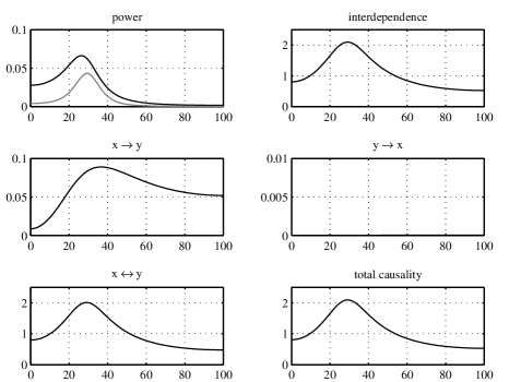
Figure 2: Simulation results for an AR(2) model consisting of two coupled time series. Power (black for $X$, gray for $Y$) spectra, interdependence spectrum (related to the coherence spectrum), and Granger causality spectra are displayed. Note that the total causality spectrum, representing the sum of directional causalities and the instantaneous causality, is nearly identical to the interdependence spectrum.

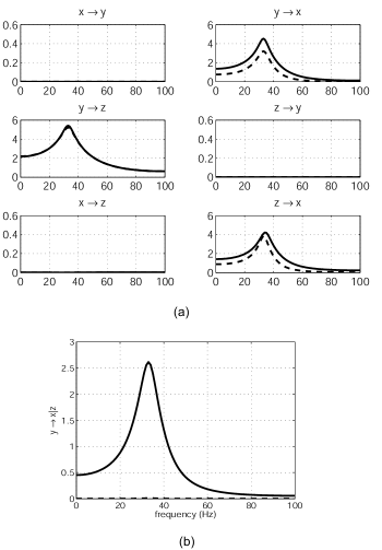
Figure 3: Simulation results for three coupled time series. Two distinct patterns of connectivity as that illustrated in Fig. 1 are considered. Results for the case with a direct causal influence are shown as solid curves and the results for the case with indirect causal influence are shown as dashed curves. (a) Pairwise Granger causality analysis gives very similar results for both cases which indicates that the pairwise analysis cannot differentiate these two patterns of connectivity. (b) Conditional causality analysis shows a nonzero spectrum (solid) for the direct case and almost zero spectrum (dashed) for the indirect case.

5.2 Example 2

Here we consider two models. The first consists of three time series simulating the case shown in Figure 1(a), in which the causal influence from $Y_{t}$ to $X_{t}$ is indirect and completely mediated by $Z_{t}$:

$$\begin{array}[]{l}X_{t}=0.8X_{t-1}-0.5X_{t-2}+0.4Z_{t-1}+\epsilon_{t}\\ Y_{t}=0.9Y_{t-1}-0.8Y_{t-2}+\xi_{t}\\ Z_{t}=0.5Z_{t-1}-0.2Z_{t-2}+0.5Y_{t-1}+\eta_{t}.\\ \end{array}$$ (145)

The second model creates a situation corresponding to Figure 1(b), containing both direct and indirect causal influences from $Y_{t}$ to $X_{t}$. This is achieved by using the same system as in Eq. (145), but with an additional term in the first equation:

$$\begin{array}[]{l}X_{t}=0.8X_{t-1}-0.5X_{t-2}+0.4Z_{t-1}+0.2Y_{t-2}+\epsilon_{t}\\ Y_{t}=0.9Y_{t-1}-0.8Y_{t-2}+\xi_{t}\\ Z_{t}=0.5Z_{t-1}-0.2Z_{t-2}+0.5Y_{t-1}+\eta_{t}.\\ \end{array}$$ (146)

For both models. $\epsilon(t),\xi(t),\eta(t)$ are three independent gaussian white noise processes with zero means and variances of $\sigma_{1}^{2}=0.3,\sigma_{2}^{2}=1,\sigma_{3}^{2}=0.2$, respectively.

Each model was simulated to generate a data set of 500 realizations of 100 time points each. First, pairwise Granger causality analysis was performed on the simulated data set of each model. The results are shown in Figure 3(a), with the dashed curves showing the results for the first model and the solid curves for the second model. From these plots it is clear that pairwise analysis cannot differentiate the two coupling schemes. This problem occurs because the indirect causal influence from $Y_{t}$ to $X_{t}$ that depends completely on $Z_{t}$ in the first model cannot be clearly distinguished from the direct influence from $Y_{t}$ to $X_{t}$ in the second model. Next, conditional Granger causality analysis was performed on both simulated data sets. The Granger causality spectra from $Y_{t}$ to $X_{t}$ conditional on $Z_{t}$ are shown in Figure 3(b), with the second model’s result shown as the solid curve and the first model’s result as the dashed curve. Clearly, the causal influence from $Y_{t}$ to $X_{t}$ that was prominent in the pairwise analysis of the first model in Figure 3(a), is no longer present in Figure 3(b). Thus, by correctly determining that there is no direct causal influence from $Y_{t}$ to $X_{t}$ in the first model, the conditional Granger causality analysis provides an unambiguous dissociation of the coupling schemes represented by the two models.

5.3 Example 3

We simulated a 5-node oscillatory network structurally connected with different delays.

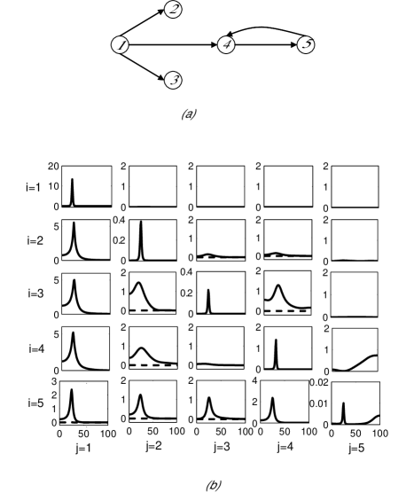
Figure 4: Simulation results for a five-node network structurally connected with different time delays. (a) Schematic illustration of the system. (b) Calculated power spectra are shown in the diagonal panels, results of pairwise (solid) and conditional Granger causality analysis (dashed) are in off-diagonal panels. Granger causal influence is from the horizontal index to the vertical index. Features of Granger causality spectra (both pairwise and conditional) are consistent with that of power spectra.

This example has been analyzed with partial directed coherence and directed transfer function methods in [12]. The network involves the following multivariate autoregressive model

$$\begin{array}[]{l}X_{1t}=0.95\sqrt{2}X_{1(t-1)}-0.9025X_{1(t-2)}+\epsilon_{1t}\\ X_{2t}=0.5X_{1(t-2)}+\epsilon_{2t}\\ X_{3t}=-0.4X_{1(t-3)}+\epsilon_{3t}\\ X_{4t}=-0.5X_{1(t-2)}+0.25\sqrt{2}X_{4(t-1)}+0.25\sqrt{2}X_{5(t-1)}+\epsilon_{4t}\\ X_{5t}=-0.25\sqrt{2}X_{4(t-1)}+0.25\sqrt{2}X_{5(t-1)}+\epsilon_{5t},\\ \end{array}$$ (147)

where $\epsilon_{1t},\epsilon_{2t},\epsilon_{3t},\epsilon_{4t},\epsilon_{5t}$ are independent gaussian white noise processes with zero means and variances of $\sigma_{1}^{2}=0.6,\sigma_{2}^{2}=0.5,\sigma_{3}^{2}=0.3,\sigma_{4}^{2}=0.3,\sigma_{5}^{2}=0.6$, respectively. The structure of the network is illustrated in Figure 4(a).

We simulated the network model to generate a data set of 500 realizations each with 10 time points. Assuming no knowledge of the model, we fitted a 5th order MVAR model on the generated data set and performed power spectra, coherence and Granger causality analysis on the fitted model. The results of power spectra are given in the diagonal panels of Figure 4(b). It is clearly seen that all five oscillators have a spectral peak at around 25Hz and the fifth has some additional high frequency activity as well. The results of pairwise Granger causality spectra are shown in the off-diagonal panels of Figure 4(b) (solid curves). Compared to the network diagram in Figure 4(a) we can see that pairwise analysis yields connections that can be the result of direct causal influences (e.g. $1\rightarrow 2$), indirect causal influences (e.g. $1\rightarrow 5$) and differentially delayed driving inputs (e.g. $2\rightarrow 3$). We further performed a conditional Granger causality analysis in which the direct causal influence between any two nodes are examined while the influences from the other three nodes are conditioned out. The results are shown as dashed curves in Figure 4(b). For many pairs the dashed curves and solid curves coincide (e.g. $1\rightarrow 2$), indicating that the underlying causal influence is direct. For other pairs the dashed curves become zero, indicating that the causal influences in these pairs are either indirect are the result of differentially delayed inputs. These results demonstrate that conditional Granger causality furnishes a more precise network connectivity diagram that matches the known structural connectivity. One noteworthy feature about Figure 4(b) is that the spectral features (e.g. peak frequency) are consistent across both power and Granger causality spectra. This is important since it allows us to link local dynamics with that of the network.

6 Analysis of a Beta Oscillation Network in Sensorimotor Cortex

A number of studies have appeared in the neuroscience literature where the issue of causal effects in neural data is examined [6, 8, 9, 10, 11, 12, 13, 14, 15]. Three of these studies [9, 10, 15] used the measures presented in this article. Below we review one study published by our group [6, 15].

Local field potential data were recorded from two macaque monkeys using transcortical bipolar electrodes at 15 distributed sites in multiple cortical areas of one hemisphere (right hemisphere in monkey GE and left hemisphere in monkey LU) while the monkeys performed a GO/NO-GO visual pattern discrimination task [16]. The prestimulus stage began when the monkey depressed a hand lever while monitoring a display screen. This was followed from 0.5 to 1.25 sec later by the appearance of a visual stimulus (a four-dot pattern) on the screen. The monkey made a GO response (releasing the lever) or a NO-GO response (maintaining lever depression) depending on the stimulus category and the session contingency. The entire trial lasted about 500 ms, during which the local field potentials were recorded at a sampling rate of 200 Hz.

Previous studies have shown that synchronized beta-frequency (15-30 Hz) oscillations in the primary motor cortex are involved in maintaining steady contractions of contralateral arm and hand muscles. Relatively little is known, however, about the role of postcentral cortical areas in motor maintenance and their patterns of interaction with motor cortex. Making use of the simultaneous recordings from distributed cortical sites we investigated the interdependency relations of beta-synchronized neuronal assemblies in pre- and postcentral areas in the prestimulus time period. Using power and coherence spectral analysis, we first identified a beta-synchronized large-scale network linking pre- and postcentral areas. We then used Granger causality spectra to measure directional influences among recording sites, ascertaining that the dominant causal influences occurred in the same part of the beta frequency range as indicated by the power and coherence analysis. The patterns of significant beta-frequency Granger causality are summarized in the schematic Granger causality graphs shown in Figure 5. These patterns reveal that, for both monkeys, strong Granger causal influences occurred from the primary somatosensory cortex ($S1$) to both the primary motor cortex ($M1$) and inferior posterior parietal cortex ($7a$ and $7b$), with the latter areas also exerting Granger causal influences on the primary motor cortex. Granger causal influences from the motor cortex to postcentral areas, however, were not observed.

Our results are the first to demonstrate in awake monkeys that synchronized beta oscillations not only bind multiple sensorimotor areas into a large-scale network during motor maintenance behavior, but also carry Granger causal influences from primary somatosensory and inferior posterior parietal cortices to motor cortex. Furthermore, the Granger causality graphs in Figure 5 provide a basis for fruitful speculation about the functional role of each cortical area in the sensorimotor network. First, steady pressure maintenance is akin to a closed loop control problem and as such, sensory feedback is expected to provide critical input needed for cortical assessment of the current state of the behavior. This notion is consistent with our observation that primary somatosensory area ($S1$) serves as the dominant source of causal influences to other areas in the network. Second, posterior parietal area $7b$ is known to be involved in nonvisually guided movement. As a higher-order association area it may maintain representations relating to the current goals of the motor system. This would imply that area $7b$ receives sensory updates from area $S1$ and outputs correctional signals to the motor cortex ($M1$). This conceptualization is consistent with the causality patterns in Figure 5. As mentioned earlier, previous work has identified beta range oscillations in the motor cortex as an important neural correlate of pressure maintenance behavior. The main contribution of our work is to demonstrate that the beta network exists on a much larger scale and that postcentral areas play a key role in organizing the dynamics of the cortical network. The latter conclusion is made possible by the directional information provided by Granger causality analysis.

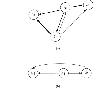
Figure 5: Granger causality graphs for monkey GE (a) and monkey LU (b).

Since the above analysis was pairwise, it had the disadvantage of not distinguishing between direct and indirect causal influences. In particular, in monkey GE, the possibility existed that the causal influence from area $S1$ to inferior posterior parietal area $7a$ was actually mediated by inferior posterior parietal area $7b$ (Figure 5(a)). We used conditional Granger causality to test the hypothesis that the ${S1\rightarrow 7a}$ influence was mediated by area $7b$. In Figure 6(a) is presented the pairwise Granger causality spectrum from $S1$ to $7a$ (${S1\rightarrow 7a}$, dark solid curve), showing significant causal influence in the beta frequency range. Superimposed in Figure 6(a) is the conditional Granger causality spectrum for the same pair, but with area $7b$ taken into account (${S1\rightarrow 7a|7b}$, light solid curve). The corresponding 99% significance thresholds are also presented (light and dark dashed lines coincide). These significance thresholds were determined using a permutation procedure that involved creating 500 permutations of the local field potential data set by random rearrangement of the trial order independently for each channel (site). Since the test was performed separately for each frequency, a correction was necessary for the multiple comparisons over the whole range of frequencies. The Bonferroni correction could not be employed because these multiple comparisons were not independent. An alternative strategy was employed following Blair and Karniski [17]. The Granger causality spectrum was computed for each permutation, and then the maximum causality value over the frequency range was identified. After 500 permutation steps, a distribution of maximum causality values was created. Choosing a p-value at $p=0.01$ for this distribution gave the thresholds shown in Figure 6(a),(b) and (c) as dashed lines.

We see from Figure 6(a) that the conditional Granger causality is greatly reduced in the beta frequency range and no longer significant, meaning that the causal influence from $S1$ to $7a$ is most likely an indirect effect mediated by $7b$. This conclusion is consistent with the known neuroanatomy of the sensorimotor cortex [18] in which area $7a$ receives direct projections from area $7b$ which in turn receives direct projections from the primary somatosensory cortex. No pathway is known to project directly from the primary somatosensory cortex to area $7a$.

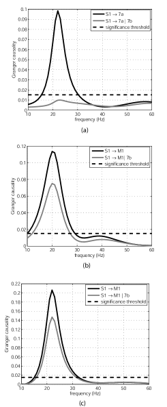
Figure 6: Comparison of pairwise and conditional Granger causality spectra for monkey GE (a and b), and monkey LU (c).

From Figure 5(a) we see that the possibility also existed that the causal influence from $S1$ to the primary motor cortex ($M1$) in monkey GE was mediated by area $7b$. To test this possibility, the Granger causality spectrum from $S1$ to $M1$ (${S1\rightarrow M1}$, dark solid curve in Figure 6(b)) was compared with the conditional Granger causality spectrum with $7b$ taken into account (${S1\rightarrow M1|7b}$, light solid curve in Figure 6(b)). In contrast to Figure 6(a), we see that the beta-frequency conditional Granger causality in Figure 6(b) is only partially reduced, and remains well above the 99% significance level. From Figure 4(b), we see that the same possibility existed in monkey LU of the $S1$ to $M1$ causal influence being mediated by $7b$. However, just as in Figure 6(b), we see in Figure 6(c) that the beta-frequency conditional Granger causality for monkey LU is only partially reduced, and remains well above the 99% significance level.

The results from both monkeys thus indicate that the observed Granger causal influence from the primary somatosensory cortex to the primary motor cortex was not simply an indirect effect mediated by area $7b$. However, we further found that area $7b$ did play a role in mediating the $S1$ to $M1$ causal influence in both monkeys. This was determined by comparing the means of bootstrap resampled distributions of the peak beta Granger causality values from the spectra of ${S1\rightarrow M1}$ and ${S1\rightarrow M1|7b}$ by the Student’s t-test. The significant reduction of beta-frequency Granger causality when area $7b$ is taken into account (t = 17.2 for GE; t = 18.2 for LU, p $<<<$ 0.001 for both), indicates that the influence from the primary somatosensory to primary motor area was partially mediated by area $7b$. Such an influence is consistent with the known neuroanatomy [18] where the primary somatosensory area projects directly to both the motor cortex and area 7b, and area 7b projects directly to primary motor cortex.

7 Summary

In this article we have introduced the mathematical formalism for estimating Granger causality in both time and spectral domain from time series data. Demonstrations of the technique’s utilities are carried out on both simulated data, where the patterns of interactions are known, and on local field potential recordings from monkeys performing a cognitive task. For the latter we have stressed the physiological interpretability of the findings and pointed out the new insights afforded by these findings. It is our belief that Granger causality offers a new way of looking at cooperative neural computation and it enhances our ability to identify key brain structures underlying the organization of a given brain function.

References

- [1] N. Wiener (1956). The theory of prediction. In: E. F. Beckenbach (Ed) Modern Mathermatics for Engineers, Chap 8. McGraw-Hill, New York.
- [2] C. W. J. Granger (1969). Investigating causal relations by econometric models and cross-spectral methods, Econometrica, 37, 424-438.
- [3] J. Geweke (1982). Measurement of linear dependence and feedback between multiple time series, J of the American Statistical Association, 77, 304-313.
- [4] J. Geweke (1984). Measures of conditional linear dependence and feedback between time series, J of the American Statistical Association, 79, 907-915.
- [5] C. Gourierous and A. Monfort (1997). Time Series and Dynamic Models, (Cambridge University Press, London)
- [6] Y. Chen, S. L. Bressler and M. Ding. Frequency decomposition of conditional Granger causality and application to multivariate neural field potential data, J. Neuroscience Method, in press.
- [7] M. Ding, S. L. Bressler, W. Yang and H. Liang (2000). Short-window spectral analysis of cortical event-related potetials by adaptive multivariate autoreggressive modelling: data preprocessing, model validation, and variability assessment, Biol. Cybern. 83, 35-45.
- [8] W. A. Freiwald, P. Valdes, J. Bosch et. al. (1999). Testing non-linearity and directedness of interactions between neural groups in the macaque inferotemporal cortex, J. Neuroscience Methods, 94, 105-119.
- [9] C. Bernasconi and P. Konig (1999). On the directionality of cortical interactions studied by structural analysis of electrophysiological recordings, Biol. Cybern., 81, 199-210.
- [10] C. Bernasconi, A. von Stein, C. Chiang and P. Konig (2000). Bi-directional interactions between visual areas in the awake behaving cat, NeuroReport, 11, 689-692.
- [11] M. Kaminski, M. Ding, W. A. Truccolo and S. L. Bressler (2001). Evaluating causal relations in neural systems: Granger causality, directed transfer function and statistical assessment of significance, Biol. Cybern. 85, 145-157.
- [12] L. A. Baccala and K. Sameshima (2001). Partial directed coherence: a new concept in neural structure determination, Biol. Cybern. 84, 463-474.
- [13] R. Goebel, A. Roebroek, D. Kim and E. Formisano (2003). Investigating directed cortical interactions in time-resolved fMRI data using vector autoregressive modeling and Granger causality mapping, Magnetic Resonance Imaging, 21, 1251-1261.
- [14] W. Hesse, E. Moller, M. Arnold and B. Schack (2003). The use of time-variant EEG Granger causality for inspecting directed interdependencies of neural assemblies, J of Neuroscience Method, 124, 27-44.
- [15] A. Brovelli, M. Ding, A. Ledberg, Y. Chen, R. Nakamura and S. L. Bressler (2004). Beta oscillatory in a large-scale sensorimotor cortical network: directional influences revealed by Granger causality, PNAS, 101, 9849-9854.
- [16] S.L. Bressler, R. Coppola and R. Nakamura (1993). Episodic multiregional cortical coherence at multiple frequencies during visual task performance, Nature, 366, 153-156.
- [17] R.C. Blair and W. Karniski (1993). An alternative method for significance testing of waveform differnce potentials, Psychophysiology, 30, 518-524.
- [18] D. J. Felleman and D. C. V. Essen (1991). Distributed hierarchical processing in the cerebral cortex, Cerebral Cortex, 1, 1-47.