Distance based Inference for
Gene-Ontology Analysis of
Microarray Experiments

Abstract

The increasing availability of high throughput data arising from gene expression studies leads to the necessity of methods for summarizing the available information. As annotation quality improves it is becoming common to rely on the Gene Ontology (GO) to build functional profiles that characterize a set of genes using the frequency of use of each GO term or group of terms in the array. In this work we describe a statistical model for such profiles, provide methods to compare profiles and develop inferential procedures to assess this comparison. An R-package implementing the methods is available.

1 Introduction

DNA microarrays belong to recently developed technologies which allow to measure the expression of thousands of genes simultaneously, in a single experiment. It is expected that these experiments will contribute to solve many relevant biological problems ranging from the identification of complex genetic diseases, Alon et al. (1999), or the prediction of tumor type, Alizadeh et al. (2000), to target discovery the pharmaceutical industry.

A common trait in these type of studies is the fact that they generate huge quantities of data and one may end with lists of up-to thousands of genes which need to be given a biological interpretation.

A typical microarray experiment is one who looks for genes differentially expressed between two or more conditions. That is, genes which behave differently in one condition (for instance healthy [or untreated or wild-type] cells) than in another (for instance tumour [or treated or mutant] cells). The study by Hengel et al. (2003) is of this type and will be used as an illustration of the ideas discussed in this paper. These authors showed that memory $CD4+$ T–cells behave differently if they present ($CD62L+$) or they lack ($CD62L-$) expression. In a study oriented to find the genetic regulation of these differences they found 144 genes to be upregulated in $CD4+/CD62L-$ T–cells relative to $CD4+/CD62L+$ T–cells. Methods such as those presented here have been developed to contribute to the biological interpretation of the resulting lists of genes. To do this they rely on the Gene Ontology, which is described in the following.

1.1 The Gene Ontology

Attempts to perform a biological interpretation of these experiments are often based on the Gene Ontology (GO), an annotation database created and maintained by a public consortium, the Gene Ontology Consortium , whose main goal is, citing their mission, to produce a controlled vocabulary that can be applied to all organisms even as knowledge of gene and protein roles in cells is accumulating and changing. The GO is organized around three principles or basic ontologies: (1) Molecular function (MF), which describes tasks performed by individual gene products such as transcription factor or ATPase activity; (2) Biological process (BP), which describes broad biological goals, such as mitosis or purine metabolism, that are accomplished by ordered assemblies of molecular functions, and (3) Cellular component (CC) describing subcellular structures, locations, and macromolecular complexes such as nucleus, telomere, and origin recognition complex. A given gene product may represent one or more molecular functions, be used in one or more biological processes and appear in one or more cellular components (see Figure 1).

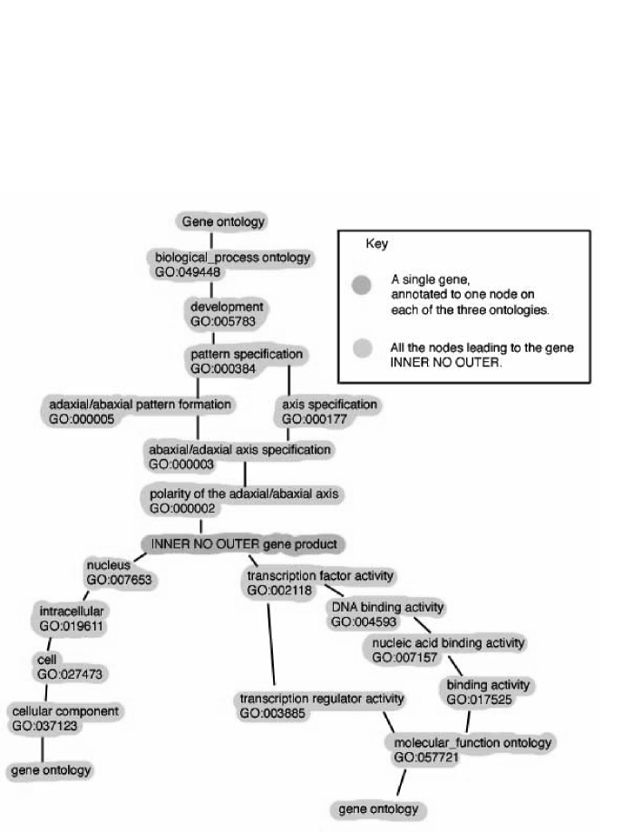
Figure 1: Networks of terms in the GO

Figure  1 shows how a given gene product can be characterized using different related terms in each ontology. An important point to note is that the information here is not “linear” in the sense that, although there is a hierarchical relation, there are interrelations between levels and terms in each ontology. As a consequence an appropriate representation for this figure is a directed acyclical graph (DAG) and several analysis methods rely precisely on this representation. This is not the case of the methods discussed here.

1.2 Summarizing and interpreting microarray experimental results

The GO is a rich data structure which contains a great quantity of information about the relation between terms. But due precisely to this, it is difficult to work with them, all at once. This fact has motivated that, in recent years, different approaches to GO–based analysis of the results of high throughput experiments have been considered. As a result of this effort many methods and even more tools have been developed. Mosquera and Sánchez-Pla (2005) is a review of the existing tools, jointly with the questions they try to solve.

Typically, after having selected one list of interesting genes one can obtain the induced sub–graph, that is the graph formed by the subset of the Gene Ontology whose nodes are related to the genes in the list, either directly or through other nodes. These graphs may be big, complex, structures, specially when the list originating them is also big. In order to simplify this structure it may be sliced or projected on the nodes which are at a certain distance of the top node (what is called a level of the GO). This will originate a table of frequencies, with each cell containing the number of genes annotated by its corresponding term at the level where the slice has been done (see Figure 2).The lattice structure of the graphs implies that one gene may appear in multiple cells of this table, which we call, from now on, a functional profile. Once this classification has been done there are different ways to analyze it which are briefly presented below.

• One straightforward possibility is to perform some type of enrichment analysis which consists of a comparison in order to establish if the percentage of genes in a certain GO category has increased or decreased in the genes selected relatively to those in the population. If this is so, a biological explanation of the differences can be attempted based on this enrichment. This is usually done by means of a Fisher test or any of its variations and is performed category-wise for each of the groups in the level selected followed by some type of multiple testing adjustment.
  Programs such as fatiGO (Al-Shahrour et al. (2004)), DAVID (Dennis et al. (2003)) and many more (see Mosquera and Sánchez-Pla (2005)) perform some form of this enrichment analysis. This is by far the most used approach nowadays.

• The main characteristic of the previous approach is the fact that each category is compared separately. A reasonable complementary extension to this may be to consider all categories at once and to compare, for instance, the categorization of selected genes with that of all the genes in the array. There exist some tools performing this type of comparisons, such as goTools, a Bioconductor package (Paquet and Yang (2005)) taking this point of view but allowing only for visual comparisons.

• Recent works are developing tests which can also be applied to analyze a whole set of genes selected a priori (see  Mootha et al. (2003) or  Smyth (2005)). Although they are related in spirit with the previous approaches, the way they proceed is totally different and will not be discussed here. A comparison seems however interesting and will be presented elsewhere.

This work is devoted to the modelling and analysis of functional profiles adopting the intermediate position just described, that is looking at the profile as a whole more than as a set of unrelated categories. It will be shown that functional profiles characterize the set of selected genes and that they can be used to perform interesting comparisons such as over-expressed vs. under-expressed genes, or between arrays of different brands.

2 Statistical models

A functional profile can be seen as a numerical vector with named cells. Each cell corresponds to a category in a given ontology, usually, but not necessarily, at the same level in the GO. Each category can be characterized by a unique number (GO:nnnnnnn) and a descriptive name. Saying that a node is at level $k$ means that the shortest path between this and the main node in each ontology (MF, BP or CC) has $k-1$ nodes. The cell number represents the number of genes whose path to the base level has a node in this category.

Table 1 shows a functional profile for a set of 140 genes clasified at the second level of the Molecular Function Ontology.

An important thing to have in mind when one considers analyzing data starting from profiles like that in Table  1 is that building this table suppresses the structure of the original data, as any categorization does and, as a result of the possibility of a gene to belong to more than one category, the sum of counts is higher than the number of genes, and in consequence a different model than the usual multinomial one is needed to represent cell counts.

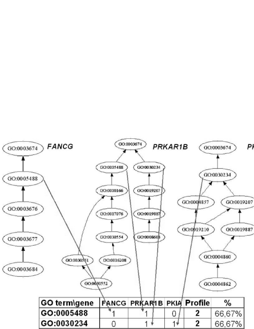
Figure 2: A simple functional profile, based only on 3 genes, showing the fact that a given gene may appear in different categories

3 The profile distribution

In order to overpass the problem that a multinomial model is not adequate to represent a functional profile, the following strategy is adopted. Given a profile with $s$ categories ($s=8$ in table  1) let $\Omega=\{A_{1},...,A_{s}\}$ be the space of events corresponding to observing one individual in one of the categories $1$,…,$s$. Given that it is possible that the same gene belongs to multiple categories we must consider, instead, the space of events

$$\Omega^{*}=\{A_{1},A_{1}\times A_{2},\dots,A_{1}\times A_{s},A_{2},A_{2}\times A_{3},\dots,A_{s-1}\times A_{s}\},$$

where $A_{i}$ means that a gene has appeared only in category $i$ and $A_{i}\times A_{j}$ means that it has appeared in both $i$ and $j$. For simplicity we make our development assuming that the multiplicity is only for two categories, but it is straightforward to extend it to more than two.

Taking this crossed-structure approach, each gene will appear only once, at most, in each category so that a given experimental situation may be characterized by an expanded profile

$$n{\mathbf{\mathcal{P}}}=n(p_{11},p_{12},...,p_{1s},...,p_{(s-1)s},p_{ss})^{t}$$ (1)

so that the sample expanded profile, $n\mathbf{\widehat{{\mathbf{\mathcal{P}}}}}$, is associated with a multinomial distribution:

$$n\mathbf{\widehat{{\mathbf{\mathcal{P}}}}}\sim{\mathbf{M}}(n;{\mathbf{\mathcal{P}}})$$ (2)

where $n$ is the number of genes forming the profile (that is, classified at a given level of a given ontology), $p_{ii}$ is the probability of a gene to belong only to class $A_{i}$, $p_{ij}=p_{ji}$ is the probability of that gene belonging simultaneously to classes $A_{i}$ and $A_{j}$ and $\hat{p}_{ii}$ and $\hat{p}_{ij}$ are the corresponding realizations from a sample of size $n$.

In practice we are interested in the distribution of the contracted variable $n\widehat{\mathbf{P}}=(n\hat{p}_{1.},n\hat{p}_{2.},...,n\hat{p}_{s.})^{t}$ which represents the profile, that is, the counts in categories $(A_{1.},A_{2.},\dots,A_{s.})$, where

$$A_{i.}=A_{i}\bigcup\left(\bigcup_{j<i}A_{j}\times A_{i}\right)\bigcup\left(\bigcup_{j>i}A_{i}\times A_{j}\right)$$

and $p_{i.}$ represents the probability of $A_{i.}$. The distribution of $n\widehat{\mathbf{P}}$ is established in the following theorem:

Theorem 1

The random variable ${n\widehat{\mathbf{P}}}=(n\hat{p}_{1.},n\hat{p}_{2.},\dots,n\hat{p}_{s.})^{t}$ is asymptotically distributed as a multivariate normal distribution

$${\mathbf{N}}(\mbox{$n\mathbf{\mu}$},n\mathbf{\Sigma}),$$

where: $\mathbb{\mu}=(p_{1.},p_{2.},\dots,p_{s.})^{t}$, and $\Sigma=(\sigma_{ij})$, with:

$$\sigma_{ii}=p_{i.}(1-p_{i.}),\ i=1,...,s,\ \sigma_{ij}=p_{ij}-p_{i.}p_{j.},i\neq j,i,j=1,...,s.$$

Proof 1

The asymptotic normality of ${n\widehat{\mathbf{P}}}$ follows from considering the asymptotic approximation of the multinomial law to the normal distribution and the distributional invariance when a linear transformation is applied to normal distributions (see Serfling (1980)), where the transformation is described by:

$$\mathbf{\widehat{{\mathbf{P}}}}=C\mathbf{\widehat{{\mathbf{\mathcal{P}}}}}$$ (3)

and $C=\left(C^{(1)}|C^{(2)}|\dots|C^{(s)}\right)$ is a matrix with $s$ rows and $s\cdot(s+1)/2$ columns defined, by boxes, as:

$$C=\left(\underbrace{\begin{array}[]{ccccc}1&1&1&\dots&1\\ 0&1&0&\dots&0\\ 0&0&1&\dots&0\\ \vdots&\vdots&\vdots&\ddots&\vdots\\ 0&0&0&\dots&1\\ \end{array}}_{C^{(1)}}\left|\underbrace{\begin{array}[]{ccccc}0&0&0&\dots&0\\ 1&1&1&\dots&1\\ 0&1&0&\dots&0\\ \vdots&\vdots&\vdots&\ddots&\vdots\\ 0&0&0&\dots&1\\ \end{array}}_{C^{(2)}}\right|\cdots\left|\underbrace{\begin{array}[]{c}0\\ 0\\ 0\\ \vdots\\ 1\\ \end{array}}_{C^{(s)}}\right.\right)$$ (4)

with

$$C^{(h)}=\left(c_{ij}^{h}\right),$$

where:

$$c_{ij}^{h}=\left\{\begin{array}[]{ll}1&\mbox{if }\ i=h\mbox{ or }(j=i-h+1\mbox{ and }i\geq h+1)\\ 0&\mbox{ elsewhere}.\end{array}\right.$$ (5)

In the following we will use the term “profile” indistinctly to refer to the absolute frequencies or to the pair formed by the relative frequencies and the number of genes, $n$.

4 Comparison of profiles

In many practical applications the user is interested in comparing profiles. This is meaningful in a variety of situations, let it be to compare the profile obtained from a set of over or under–expressed genes with all the genes on the array, to compare the profiles obtained in different experimental conditions or to compare the profiles corresponding to arrays of different types or brands.

Our approach is based on defining an appropriate measure of distance between profiles $d({\mathbf{P}_{i}},{\mathbf{P}_{j}})$. This allows to state the problem of comparing two profiles in terms of testing the hypothesis $H_{0}:\,d({\mathbf{P}_{i}},{\mathbf{P}_{j}})=0$ vs $H_{1}:\,d({\mathbf{P}_{i}},{\mathbf{P}_{j}})>0$.

The choice of the appropriate distance is often a point for extensive discussion. Sometimes the underlying statistical model is relevant for its choice. In other cases the availability, or even computational feasibility is decisive. Here we will use the squared Euclidean distance which offers a good balance between ease of interpretation and properties that can be derived for it.

One may consider different scenarios for working with this problem:

• One–sample problems consist of comparing an estimated profile with a fixed one, which makes the role of “population”. This may be, for instance, a profile obtained from the whole array or even the genome of the species if it is available.

• Two–sample problems consist of comparing two (or more) estimated profiles, which are obtained from populations which may be or may not be independent. This may be for instance the case of profiles formed with the genes selected in two different experiments about the same disease, or those obtained with the genes selected from two (or more) different mutations of a given wild type.

Only the first case will be discussed in the following. Two sample problems will be presented elsewhere.

4.1 Main results

Let ${\mathbf{P}}_{0}$ represent a fixed population profile, and $\hat{\mathbf{P}}$, an estimated profile based on a sample of size $n$. The squared Euclidean distance between ${\mathbf{{\mathbf{P}}}_{0}}$ and ${\mathbf{\hat{\mathbf{P}}}}$ is defined as:

$$d({\mathbf{\hat{\mathbf{P}}},{\mathbf{P}}_{0}})=\left(\hat{\mathbf{P}}-{\mathbf{P}}_{0}\right)^{t}\left(\hat{\mathbf{P}}-{\mathbf{P}}_{0}\right)=\sum_{i=1}^{s}(\hat{p}_{i.}-p_{i0})^{2}.$$ (6)

Based on Theorem 1, the distribution of the distances can be established setting the basis to perform statistical inference on the estimated profiles.

Theorem 2

Let ${\mathbf{P}}_{0}$ represent a fixed population profile, $\hat{\mathbf{P}}$ an estimated profile based on a sample of size $n$ and $d(\hat{\mathbf{P}},{\mathbf{P}}_{0})$ the squared Euclidean distance between ${\mathbf{{\mathbf{P}}}_{0}}$ and ${\mathbf{\hat{\mathbf{P}}}}$,

1. If ${\mathbf{P}}\neq{\mathbf{P}}_{0}$ then
   

   $$n^{1/2}\left[d(\hat{\mathbf{P}},{\mathbf{P}}_{0})-d\ ({\mathbf{P}},{\mathbf{P}}_{0})\right]\buildrel\mathcal{L}\over{\longrightarrow}{\mathbf{Z}}\sim{\mathbf{N}}(0,{\sigma^{2}}),$$ (7)

   where:

   $$\sigma^{2} = 4\,\sum_{i,j=1}^{s}(p_{i.}-p_{i0})\left(\delta_{ij}p_{i.}+(1-\delta_{ij})p_{ij}-p_{i.}p_{j.}\right)(p_{j.}-p_{j0})$$ (8)

   $$= 4({\mathbf{P}}-{\mathbf{P}}_{0})^{t}\mathbf{\Sigma}({\mathbf{P}}-{\mathbf{P}}_{0}),$$

   and “$\buildrel\mathcal{L}\over{\longrightarrow}$” stands for “convergence in distribution”.

2. If ${\mathbf{P}}={\mathbf{P}}_{0}$ then

   $$n\,d(\hat{\mathbf{P}},{\mathbf{P}}_{0})\buildrel\mathcal{L}\over{\longrightarrow}{\sum_{i=1}^{s}}\beta_{i}\chi^{2}_{1,i},$$ (9)

   where $\beta_{i}$ are the eigenvalues of matrix $\Sigma$ defined in Theorem  1 and $\chi^{2}_{1,i}$ are independent chi-squared random variables with one degree of freedom.

Proof 2

Consider the algebraic relation:

$$d(\hat{\mathbf{P}},{\mathbf{P}}_{0}) = \left(\hat{\mathbf{P}}-{\mathbf{P}}_{0}\right)^{t}\left(\hat{\mathbf{P}}-{\mathbf{P}}_{0}\right)$$ (10)

$$= \left((\hat{\mathbf{P}}-{\mathbf{P}})-({\mathbf{P}}_{0}-{\mathbf{P}})\right)^{t}\left((\hat{\mathbf{P}}-{\mathbf{P}})-({\mathbf{P}}_{0}-{\mathbf{P}})\right)$$

$$= d(\hat{\mathbf{P}},{\mathbf{P}})+d({\mathbf{P}},{\mathbf{P}}_{0})+2({\mathbf{P}}-{\mathbf{P}}_{0})^{t}(\hat{\mathbf{P}}-{\mathbf{P}}).$$

Note also that the asymptotic distribution of $n\,d(\hat{\mathbf{P}},{\mathbf{P}})$ follows from standard results about quadratic forms (Dik and Gunst (1985)):

$$n\ d(\hat{\mathbf{P}},{\mathbf{P}})=n\ (\hat{\mathbf{P}}-{\mathbf{P}})^{t}\mathbb{I}_{s}(\hat{\mathbf{P}}-{\mathbf{P}})\buildrel\mathcal{L}\over{\longrightarrow}{\sum_{i=1}^{s}}\beta_{i}\chi^{2}_{1,i},$$ (11)

where $\mathbb{I}_{s}$ is the $s-$dimensional identity matrix and $\beta_{i}$ are the eigenvalues of $\mathbb{I}_{s}\Sigma=\Sigma$.

The proof of Theorem 2 is based on some properties of the squared Euclidean distance. It can be easily extended to other smooth distance indexes with the only condition that they admit a Taylor series expansion. In that case the approximation appearing in (11) would be based on the eigenvalues of $H_{T}\Sigma$ where $H_{T}$ is the Taylor Hessian of the distance expansion. It must be noted, however, that with squared Euclidean distance, error terms depend exclusively on the convergence of the multinomial to the normal distribution given that terms of order greater than two vanish in the Taylor expansion. In absence of other constrains, such as biological interpretation, this is an additional argument favoring the use of this distance in front of other options.

In practical situations it is often difficult to deal with linear combinations of chi–squared random variables. Rao and Scott (1981) suggested to use the following approximation for the combination introduced in equation  9:

$${\sum_{i=1}^{s}}\beta_{i}\chi^{2}_{1,i}\simeq\overline{\beta}\chi^{2}_{rank\Sigma}$$ (14)

where

$$\overline{\beta}=\frac{1}{s}\left[\sum_{i=1}^{s}p_{io}(1-p_{io})\right],$$

and $\chi^{2}_{rank\Sigma}$ stands for a chi–square random variable with $rank\Sigma$ degrees of freedom.

Our simulation results show that the above approximation performs very poorly in our case. In this work we have used a similar approximation which we consider to have better adaptability properties:

$$\sum_{i=1}^{s}\beta_{i}\chi^{2}_{1,i}\simeq a\chi^{2}_{rank\Sigma}+b,$$ (15)

where

$$E\left(\overline{\chi}_{\beta}^{2}\right)=a\,E\left(\chi^{2}_{rank\Sigma}\right)+b\quad\mbox{and}\quad Var\left(\overline{\chi}_{\beta}^{2}\right)=a^{2}\,Var\left(\chi^{2}_{rank\Sigma}\right)$$ (16)

giving:

$$a=\sqrt{\sum_{i=1}^{s}\beta_{i}^{2}}\quad\mbox{and}\quad b=\sum_{i=1}^{s}\beta_{i}-\sqrt{s\,\sum_{i=1}^{s}\beta_{i}^{2}}.$$ (17)

4.2 Applications

These results make it possible to construct hypothesis tests and confidence intervals to perform statistical inference on the profiles.

An approximate confidence interval for the “true” distance $d\left({{\rm{\bf P}},{\rm{\bf P}}_{0}}\right)$, with approximate confidence level $1-2\alpha$ is

$$\left[{d(\hat{\mathbf{P}},{\mathbf{P}}_{0})-z_{\alpha}\frac{\hat{\sigma}}{\sqrt{n}}\,{\kern 1.0pt},\quad d(\hat{\mathbf{P}},{\mathbf{P}}_{0})+z_{\alpha}\frac{\hat{\sigma}}{\sqrt{n}}}\right]$$ (18)

where $\hat{\sigma}=2\sqrt{\left({{\rm{\bf\hat{P}}}-{\rm{\bf P}}_{0}}\right)^{t}\hat{\Sigma}\left({{\rm{\bf\hat{P}}}-{\rm{\bf P}}_{0}}\right)}$ is the sample standard error estimator of $n\,d(\hat{\mathbf{P}},{\mathbf{P}}_{0})$, directly obtained from (8), and $z_{\alpha}$ stands for the $\alpha$ right quantile of a standard normal random variable $Z$, $\Pr\left\{{Z\geqslant z_{\alpha}}\right\}=\alpha.$

Consider now the contrast

$$\begin{array}[]{l}H_{0}:\quad d({\mathbf{P}},{\mathbf{P}}_{0})=0\\ H_{1}:\quad d({\mathbf{P}},{\mathbf{P}}_{0})>0\\ \end{array}$$ (19)

(Say, is the set of differentially expressed genes enriched/impoverished in some GO categories with respect to all the genes in the array?) From (7) the rule

$$\mbox{``Reject $H_{0}$ if }P\left(\sum_{i=1}^{n}\beta_{i}\chi_{1i}^{2}\geq n\hat{d}\right)\leq\alpha\mbox{''},$$ (20)

defines a test of nominal size $\alpha$ where $\hat{d}$ stands for the sample squared euclidean distance value.

There exist approximate methods to compute tail probabilities of linear combinations of independent chi–square random variables. See Sheil and O’Muircheartaigh (1977) for the case of non–negative coefficients or Farebrother (1984) for more general algorithms.

These algorithms are computationally complex so that we have taken a more direct approach based on simulation. It consists of estimating the probability in (20) by means of the relative frequency

$$\frac{\#[Y_{j}\geq n\hat{d}]}{m},$$

where $Y_{j},\ j=1,\dots,m$, are independent realizations of $\sum_{i=1}^{n}\beta_{i}\chi_{1i}^{2}$.

In the examples and simulations described in the next sections, we have taken $m$ = 10,000.

Similarly, the rule

$$\mbox{``Reject $H_{0}$ if }\ P\left(\chi_{rank\Sigma}^{2}\geq\frac{n\hat{d}-b}{a}\right)\leq\alpha\mbox{''},$$ (21)

defines an alternative test procedure. Here $a$ and $b$ are defined in (17). This last method is slightly easier to compute as no simulations nor complex approximations are required to obtain the critical value. Note that $\Sigma$ used in the test procedures is the known covariance matrix associated to the known profile specified by the null hypothesis.

5 Example. Biological interpretation of a list of genes

$CD4+$ T–cells are a type of white-blood cells which are very important in the organism immune surveillance. As an example of the many processes in which they are involved it is known that the decrease in number of $CD4+$ T–cells is the primary mechanism by which HIV causes AIDS. The activation of T–cells is related to the presence of a substance, L-selectin ($CD62L$). This molecule may be absent or present in a cell yielding two possible types of cells: $CD4+/CD62L-$ T–cells lack L–selectin expression, whereas $CD4+/CD62L+$ T–cells present L–selectin expression.

Hengel et al. (2003) performed a study aiming at finding the genetic regulation of these differences. They found 144 genes to be up–regulated in $CD4+/CD62L-$ T–cells relative to $CD4+/CD62L+$ T–cells. The list is available in the supplementary material website. All the computations in this work have used only 140 of these genes, because there are 4 which were not annotated in the GO.

Table 1 shows the functional profiles for this list of genes at the first level of the three ontologies.

There are two reasons why these profiles are not necessarily very informative. First, for simplicity, we have built the profile at the highest possible level formed by very generic groups. Even if these functionalities are too general one might rely on them for interpretation, but first we need to know if this profile characterizes the selected genes or it is simply the profile corresponding to the population, or in this case, to a big sub–population formed by all the genes in the microarray. In order to answer this second question a comparison of profiles is meaningful. Figure 3 and table 2 show the comparison between the sample (140 genes in the list) and the population (all the genes on the chip) profiles. It can be seen that there does not appear to be any significant difference in BP and MF profiles, but there is some for Cellular Component.

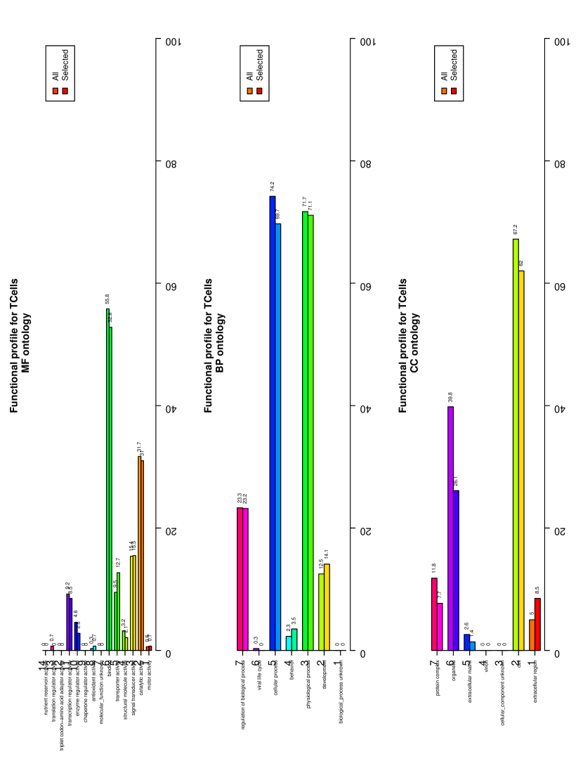
Figure 3: comparison of GO profiles for all three ontologies at level one of these 140 genes relative to all the genes in the array (hgu95A)

Table  2 shows the distances and p–values computed using the two methods described above. The test performed here has null hypothesis $H_{0}:d({\mathbf{P}},{\mathbf{P}}_{0})=0$, that is, not rejecting the null hypothesis means that the set of genes considered to be differentially expressed is distributed between GO categories in the same form as all the genes in the array.

Description	GOID	Frequency
catalytic activity	GO:0003824	38
signal transducer activity	GO:0004871	21
structural molecule activity	GO:0005198	2
transporter activity	GO:0005215	16
binding	GO:0005488	76
antioxidant activity	GO:0016209	1
enzyme regulator activity	GO:0030234	4
transcription regulator activity	GO:0030528	10
Total number of hits		168

Table 1: Functional profiles at the first level of the Molecular Function Ontology for the list of genes in the example data

Ontology	Distance $\pm$ precision	LC-chi p-value	Approx-chi p-value
MF	0.00734 $\pm$ 0.013114	0.5744	0.6062
BP	0.00511 $\pm$ 0.009710	0.4112	0.4611
CC	0.05749 $\pm$ 0.053666	0.0000	3.11e-07

Table 2: Distances and p–values computed on first–level profiles for the three ontologies for the example data. “LC-chi” stands for the test based on linear combinations of chi–square random variables (20) and “Approx–chi” stands for the test based on approximating a chi–square distribution (21)

6 Simulation studies

The accuracy of the preceding results and methods has been tested by simulation. The simulated scenarios emulate the case of $CD4+/CD62L+$ T–cells discussed in previous sections. Each simulation was characterized by three main parameters: a sample size $n$ and two expanded profiles ${\mathbf{\mathcal{P}}}$ and ${\mathbf{\mathcal{P}}}_{0}$ which induced the profiles ${\mathbf{P}}=C{\mathbf{\mathcal{P}}}$ and ${\mathbf{P}}_{0}=C{\mathbf{\mathcal{P}}}_{0}$.

For each one of the simulation scenarios characterized by a given combination of the above parameters, 10,000 (expanded) sample profiles were generated according to a multinomial distribution $\mathbf{M}({\mathbf{\mathcal{P}}};n)$ and contracted according to (3). For each generated profile, the test procedures (20) and (21) were applied in order to determine whether the null hypothesis in (19) was rejected or not, and the confidence interval (18) computed to determine its length and to inspect its coverage of the true distance $d\left({{\rm{\bf P}},{\rm{\bf P}}_{0}}\right)$. These simulation results were collected to estimate the true rejection probabilities, the mean interval length and the true coverage probability.

In a first series of simulation experiments, the profiles specified in the preceding example were taken as directly defining the population and/or the null hypothesis, with $n$ = 140.

Table  3 displays the (simulation estimated) probability of rejecting $H_{0}$, the mean length of the confidence interval and its coverage. All results correspond to a nominal significance level of 0.05 or to a nominal coverage of 0.95.

				Profile specifying $H_{0}$
			Onto	CD62L	hgu95A
Simulated profiles	CD62L		BP	0.0483$\pm$0.0042
		LC–chi	MF	0.0439$\pm$0.0040
			CC	0.0475$\pm$0.0042
			BP	0.0529$\pm$0.0044
		Approx–chi	MF	0.0524$\pm$0.0044
			CC	0.0475$\pm$0.0042
			BP	0.0178$\pm$7.58E-5
		Interval length	MF	0.0220$\pm$8.59E-5
			CC	0.0092$\pm$7.01E-5
			BP	0.9951$\pm$0.0014
		Coverage	MF	0.9883$\pm$0.0021
			CC	0.9986$\pm$0.0007
	hgu95A		BP	0.1397$\pm$0.0068	0.0527$\pm$0.0044
		LC–chi	MF	0.3555$\pm$0.0094	0.0550$\pm$0.0045
			CC	0.9057$\pm$0.0057	0.0453$\pm$0.0041
			BP	0.1455$\pm$0.0069	0.0557$\pm$0.0045
		Approx–chi	MF	0.3692$\pm$0.0095	0.0574$\pm$0.0046
			CC	0.9198$\pm$0.0053	0.0518$\pm$0.0043
			BP	0.0215 $\pm$8.63E-5	0.0183$\pm$7.89E-5
		Interval length	MF	0.0292$\pm$8.97E-5	0.0215$\pm$ 8.65E-5
			CC	0.0313$\pm$ 0.0001	0.0042$\pm$3.37E-5
			BP	0.9907$\pm$0.0019	0.9943$\pm$0.0015
		Coverage	MF	0.9794$\pm$0.0028	0.9868$\pm$0.0022
			CC	0.8896$\pm$0.0061	0.9842$\pm$0.0024

Table 3: Probability of rejecting $H_{0}$, mean length of the confidence interval for the true squared Euclidean distance and coverage. Simulated profiles were generated according to CD62L or hgu95A. All simulation results are displayed with $\pm$95% confidence limits. “LC–chi” stands for the test based on linear combinations of chi–square random variables (20) and “Approx–chi” stands for the test based on approximating a chi–square distribution (21)

$H_{0}$ is true when the profile generating the gene samples and the profile specifying $H_{0}$ are the same. In these cases, both tests seem to perform according to the nominal significance level, with an apparent tendency of test (21) to slightly higher type I error probabilities. As can be expected, the confidence interval (18) is not adequate when $H_{0}$ is true, with a greater coverage than the nominal one and a low precision (the intervals are too long in mean). When ${\mathbf{P}}_{0}$ corresponds to CD62L and ${\mathbf{P}}$ to hgu95A, $H_{0}$ is not true, though both profiles are very similar in the BP and MF ontologies, with “true” squared Euclidean distances of 0.0020 and 0.0064, respectively. For $n$ = 140, the power of the tests is low, around 0.14 for BP and 0.36 for MF. That is, for these quite similar “true” profiles, the probability of type II error is high and the confidence interval still performs not adequately. On the other hand, the simulated profiles differ appreciably more for the CC ontology. Then the power of the tests is much greater, around 0.91, but the coverage is still inadequate, now too low.

In order to have a more comprehensive view, we performed an additional simulation study. The following geometric model was considered:

Let ${\mathbf{\mathcal{P}}}=\left({p_{11},p_{22},\ldots,p_{ss},p_{12},p_{13},\ldots,p_{(s-1)s},p_{123},\ldots}\right)^{t}$ represent an expanded profile. Maintaining the order of the elements, recode the indexes as

$$\left({p_{[1]},p_{[2]},\ldots,p_{[s]},p_{[s+1]},p_{[s+2]},\ldots,p_{\left[{\frac{s\left({s+1}\right)}{2}}\right]},p_{\left[{\frac{s\left({s+1}\right)}{2}+1}\right]},\ldots}\right)$$

and assume that

$$p_{[i]}\propto\left({1-\theta}\right)^{i-1},\mbox{ for }0<\theta<1.$$ (22)

The sole purpose of model (22) is to define families of profiles fully characterized by a unique parameter $\theta$, for a given number of ontology classes $s$ and a given maximum level of possible simultaneity $k$ –that is, with the last term having index $\left({s-k+1}\right)\left({s-k+2}\right)\ldots\left({s-1}\right)s$. Progressively different values of $\theta$ produce progressively greater distances between profiles, that is, scenarios progressively distant from the assumption of validity of the null hypothesis. In all the simulations, $H_{0}$ was defined by a profile associated to $\theta_{0}$ = 0.4, while $\theta$ = 0.4, 0.35, 0.30, 0.25 and 0.20 defined possible scenarios were the sample profiles were generated according to distributions more and more distant from $H_{0}$. Additionally, the following sample sizes (number of genes) were considered: $n$ = 50, 100, 140, 200, 500 and 1000. Here we report the results for $s$ = 6 and $k$ = 5 (as in the $CD4+/CD62L$ T-cells example for the BP ontology) for a nominal significance level of 0.05 and nominal coverage of 0.95. The results of other situations (including $s$ = 11, $k$ = 6 and $s$ = 4, $k$ = 2, respectively the case of the MF and CC ontologies) are accessible in the supplementary documentation web site.

Figures 4 and 5 display the power curves of both tests under consideration. They perform in a very similar way and always seem to be in conformity with the nominal significance level. Thus, the test based on the chi-square approximation seems to be preferable due to its simplicity.

Figure 4: Power of the test based on linear combinations of chi–square random variables. The bottom horizontal line corresponds to the reference 0.05 significance level.

Figure 5: Power of the approximated chi-square test. The bottom horizontal line corresponds to the reference 0.05 significance level.

Figure 6 corresponds the coverage of the asymptotic confidence interval (18). As is expected, this confidence interval is not adequate under true $H_{0}$. When $H_{0}$ is false, only for large sample sizes (500 or more genes) its true coverage approximates the nominal one. Otherwise the true coverage is larger than the nominal, but at the cost of a very low precision (that is, too long intervals) as is shown in Figure 7. For example, if $n$ = 50 genes, with a true 0.005 distance, a (nominally) 95% confidence interval will have a length of approximately 0.04, too wide with respect to the magnitude of the distance.

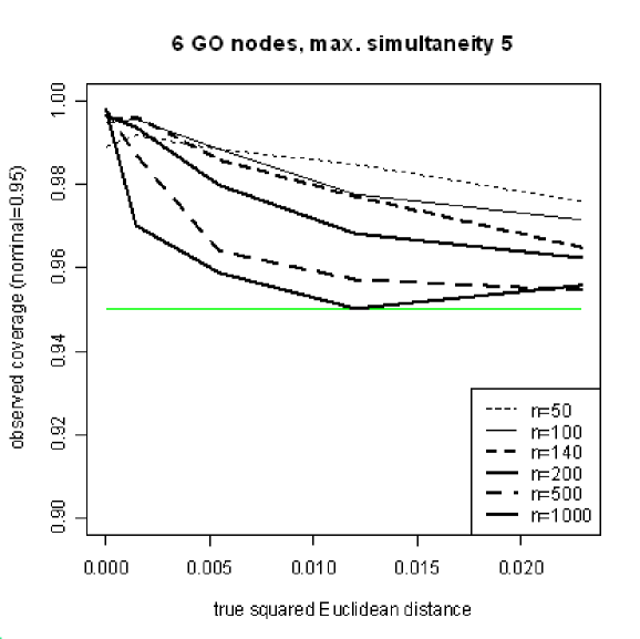
Figure 6: Coverage of the asymptotic confidence interval. The base reference line corresponds to a 0.95 coverage.

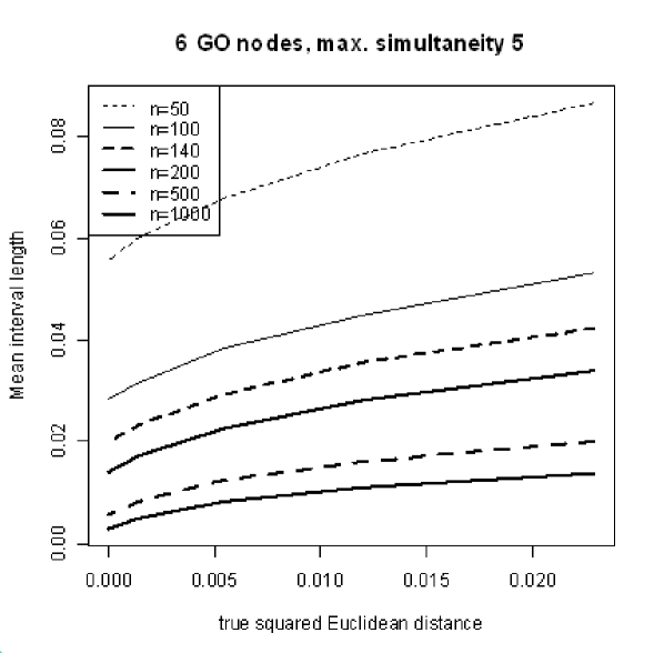
Figure 7: Mean confidence interval length

7 Discussion and Conclusion

The analysis and interpretation of biological data based on the Gene Ontology is an active field of research.

Functional profiles constitute an intuitive way to summarize sets of genes of any size to facilitate biological interpretation.

Our theoretical results set the basis for doing statistical inference based on these profiles. This allows to turn the analysis of profiles from a simple graphical comparison, such as is done in many papers (Beltran et al. (2003)) or in the goTools Bioconductor package (Paquet and Yang (2005))– to well based inferential procedures with a known degree of confidence.

Essentially we have considered global comparisons between profiles at fixed levels of the GO, but extensions are straightforward. For instance, profiling may be performed on any set of reference categories, not necessarily a fixed level. Also, the theory can be easily adapted to other situations such as the analysis of multiple response items in surveys.

The approach is, of course, not free from limitations. Profiling, as any other summary, implies a certain loose of information. Comparing the approach with the use of the whole graph it is clear that the later has more information but is more difficult to summarize. If we go in the other direction, a category by category analysis (“a la fatiGO”) helps to see what happens in specific interesting categories but does not offer a global approach. In brief our approach tries to stay between one and the other in a useful way.

7.1 Software and tools

The main applied interest of this work is to provide the genomic community a research tool that help to assess their conclusions, allowing to go one step further than visual approximations such as that offered by some programs, such as the Bioconductor package goTools (Paquet and Yang (2005)).

To facilitate the application of our results we have developed a tool which is available as an R package which will be freely accessible to the user’s community. This will also be submitted to Bioconductor to help its diffusion. Also, a web site to make the software available through the web is in development.

Acknowledegments

We are grateful to Dr. Sandrine Dudoit, at U.C. Berkeley, for her comments and support during Dr. Alex Sánchez’s stay in Berkeley, where this work was initiated.

References

- Al-Shahrour et al. (2004) Al-Shahrour, F., Diaz-Uriarte, R., Dopazo, J., 2004. FatiGO: a web tool for finding significant associations of gene ontology terms with groups of genes. Bioinformatics 20, 578–580.
- Alizadeh et al. (2000) Alizadeh, A., Eisen, M., Ma, E. D. C., , Lossos, I., Rosenwald, A., Boldrick, J., Sabet, H., Tran, T., Yu, X., Powell, J., Yang, L., Marti, G., Jr, J. H., Lu, L., Lewis, D., Tibshirani, R., Sherlock, G., Chan, W., Greiner, T., Weisenburger, D., Armitage, J., Warnke, R., Levy, R., Wilson, W., Grever, M., Byrd, J., Botstein, D., Brown, P., Staudt, L., February 2000. Distinct types of diffuse large B–cell lymphoma identified by gene expression profiling. Nature 403, 503–511.
- Alon et al. (1999) Alon, U., Barkai, N., Notterman, D., Gish, K., Ybarra, S., Mack, D., Levine, A., 1999. Broad patterns of gene expression revealed by clustering analysis of tumor and normal colon tissues probed by oligonucleotide arrays. Proceedings of the National Academy of Sciences 96, 6745–6750.
- Beltran et al. (2003) Beltran, S., Blanco, E., Serra, F., Perez-Villamil, B., Guigó, R., Artavanis-Tsakonas, S., Corominas, M., 2003. Transcriptional network controlled by the trithorax- group gene ash2 in drosophila melanogaster genome research. Proceedings of the National Academy of Sciences 100, 3293–3298.
- Dennis et al. (2003) Dennis, G. J., Sherman, B., Hosack, D., Yang, J., Baseler, M. W., Clifford Lane, H., Lempicki, R., 2003. David: Database for annotation, visualization, and integrated discovery. Genome Biology 4, P3.
- Dik and Gunst (1985) Dik, J., Gunst, M., 1985. The distribution of general quadratic forms in normal variables. Statistica Neerlandica 39, 14–26.
- Farebrother (1984) Farebrother, R., 1984. The distribution of linear combinations of random variables. Appl. Statist. 33, 366–369.
- Hengel et al. (2003) Hengel, R., Thaker, V., Pavlick, M., Metcalf, J., Dennis, G. J., Yang, J., Lempicki, R., Sereti, I., Lane, H., 2003. L-selectin (cd62l) expression distinguishes small resting memory cd4+ t cells that preferentially respond to recall antigen. J. Immunol. 170, 28–32.
- Mootha et al. (2003) Mootha, V., Lindgren, C., Eriksson, K., Subramanian, A., Sihag, S., Lehar, J., Puigserver, P., Carlsson, E., Ridderstrale, M., Laurila, E., Houstis, N., Daly, M., Patterson, N., Mesirov, J., Golub, T., Tamayo, P., Spiegelman, B., Lander, E., Hirschhorn, J., Altshuler, D., Groop, L., 2003. Pgc-1alpha-responsive genes involved in oxidative phosphorylation are coordinately downregulated in human diabetes. Nature Genet. 34, 267–73.
- Mosquera and Sánchez-Pla (2005) Mosquera, J.-L., Sánchez-Pla, A., 2005. A comparative study of go mining programs. In: X Conferencia Española de Biometría. Sociedad Española de Biometría.
-
Paquet and Yang (2005)
Paquet, A., Yang, Y., 2005. Getting started with goTools package.
URL http://bioconductor.org/repository/devel/vignette/goTools.pdf - Rao and Scott (1981) Rao, J., Scott, A., 1981. The analysis of categorical data from complex sample surveys: chi-squared tests for goodness of fit and independence in two way tables. JASA 76, 221–3.
- Serfling (1980) Serfling, R., 1980. Approximation Theorems of Mathematical Statistics. John Wiley, New York.
- Sheil and O’Muircheartaigh (1977) Sheil, J., O’Muircheartaigh, I., 1977. Algorithm AS106. The distribution of non-negative quadratic forms in normal variables. Appl. Statist. 26, 92–98.
- Smyth (2005) Smyth, G., 2005. Bioinformatics and Computational Biology Solutions using R and Bioconductor. Springer, New York, Ch. Limma: linear models for microarray data, pp. 397–420.