A variational approach to the stochastic aspects of cellular signal transduction

Abstract

Cellular signaling networks have evolved to cope with intrinsic fluctuations, coming from the small numbers of constituents, and the environmental noise. Stochastic chemical kinetics equations govern the way biochemical networks process noisy signals. The essential difficulty associated with the master equation approach to solving the stochastic chemical kinetics problem is the enormous number of ordinary differential equations involved. In this work, we show how to achieve tremendous reduction in the dimensionality of specific reaction cascade dynamics by solving variationally an equivalent quantum field theoretic formulation of stochastic chemical kinetics. The present formulation avoids cumbersome commutator computations in the derivation of evolution equations, making more transparent the physical significance of the variational method. We propose novel time-dependent basis functions which work well over a wide range of rate parameters. We apply the new basis functions to describe stochastic signaling in several enzymatic cascades and compare the results so obtained with those from alternative solution techniques. The variational ansatz gives probability distributions that agree well with the exact ones, even when fluctuations are large and discreteness and nonlinearity are important. A numerical implementation of our technique is many orders of magnitude more efficient computationally compared with the traditional Monte Carlo simulation algorithms or the Langevin simulations.

I Introduction

The life of the cell is regulated by intricate chains of chemical reactions st02gomp . The whole cell may be viewed as a computing device where information is received, relayed and processed den95p . Signal transduction cascades based on protein interactions regulate cell movement, metabolism and division st02gomp ; mol02alb . Since cells are mesoscopic objects, understanding the role of the intrinsic fluctuations of the biochemical reactions as well as environmental fluctuations is a fundamental part of understanding signaling dynamics paul00st ; tan04mod ; sh05noise ; bark99cir ; kurt95st ; el02st ; sw02in ; oz02reg ; bla03noi ; wein05st ; muk04st ; rao02n . In this regard, the well-organized behavior of cells, which emerges as a result of biochemical reaction dynamics involving hundreds of cross-linked signaling pathways, is remarkable han01ex ; nick04ph ; h03ecoli ; coh05fl ; keen01df ; lem05st ; kul04pat . The problem of how signals can be precisely detected, smoothly transduced and reliably processed under noisy conditions is a research topic of great current interest, that, in turn, should lead to deeper understanding of the origins of the cell’s functional responses math02hei ; opt04cha . Furthermore, these studies can help to unravel the design principles for various signaling pathways, leading, eventually, to better ways to control and efficiently interfere with cellular activity, as would be needed to correct the behavior of diseased cells keen05len ; h03ecoli .

The role of noise in gene regulatory networks has been identified as a key issue and has been intensively studied in recent years th01in ; kie01eff ; th01st ; sw02in ; oz02reg ; bla03noi ; sasai03stch ; walcz04stgn ; jas04fl . Linearization of the noise may be acceptable if the dynamics near steady states is being studied th01in ; jas04fl ; sw02in . When protein numbers are large and, thus, the continuous approximation is valid, time-dependent distributions have been determined using the Langevin or Fokker-Planck equations  muk02att ; sw04eff ; sh05noise . To account for the discreteness in the linearized equations, the generating function approach has also been used th01in ; sw02in . A variational treatment of steady state stability and switching in nonlinear, discrete gene regulatory processes has been reportedsasai03stch ; walcz04stgn .

In cytosolic signal transduction processes, in contrast to gene transcription which involves a unique DNA molecule, all the reacting species are present in multiple copies and participate in unary, binary or perhaps even higher order reactions. Noise could be multiplicative van92st ; fox86fun and the linear description easily breaks down. Moreover, cellular reactions usually take place heterogeneously in space The localization and compartmentalization of protein organelles require diffusive or active transportation of reacting molecules from one region to another. Spatial coordination combined with temporal coordination generates coherent, yet complex spatiotemporal patterns hol05st ; coh05fl ; ku01sel ; keen01df ; lem05st ; kul04pat ; h03ecoli ; sh02mod .

The extracellular ligands often trigger cascades of chemical reactions which propagate inside a cell and induce responses from various environmental cues. The cell body is a highly heterogeneous entity and never settles to a steady state. To understand cell dynamical processes, an explicitly time-dependent description is required. Within a volume with linear dimensions of the Kuramoto length van92st ; kur74eff , diffusion mixes the reagents in a nearly uniform manner. If the reactions are considered in the Kuramoto volume, it is reasonable to neglect the spatial heterogeneity. For many signal transduction networks, however, it is likely that only a few proteins are present in the Kuramoto volume (determined by specific reaction and diffusion rates), and, therefore, the continuous description of protein numbers breaks down. To characterize stochastic signaling reactions in this volume, a time-dependent description of a noisy, discrete, nonlinear system is required lan1cas . In many situations, such as Drosophila oogenesis, the exact shape of the probability distribution profile is very important and determines different developmental paths sh02mod ; yak05sys . In the following, we discuss efficient techniques to compute the time-dependent protein number probability distributions in biochemical reaction networks when the number of protein copies is small.

The Gillespie algorithm provides an effective Monte Carlo technique for simulating stochastic chemical reactions gill77ext ; gil01app ; jer05sim . Each simulation gives a reaction trajectory which is close to the deterministic trajectory in the large particle number limit. To get well-converged statistics, many trajectories may be needed, often on the order of $10^{5}$. If there is a separation of time scales of the constituent chemical reactions, Gillespie simulations also become exceedingly slow since the reaction events are dominated by the fastest reactions while the observables typically involve the slowest reactions. Although considerable progress has been made in accelerating such simulations e05nest ; muk02att ; sw04eff ; sh05noise , computational inefficiency continues to be an impediment, especially for the spatially inhomogeneous generalization of the Gillespie algorithm. Furthermore, it is hard to extract the analytical structure of the solution from the numerical results, which can be important for achieving a deeper physical understanding of the system behavior when the rate parameters are widely varied.

Mathematically, a stochastic process may be completely characterized by a master equation - a group of ordinary differential equations (ODEs) describing the evolution of probabilities van92st ; gar02han . The main difficulty in solving a chemical master equation is the enormous number of ODEs involved even for a small reaction cascade. A number of analytical techniques have been developed for solving approximately the master equation th01st ; th01in ; sw02in . In this work, we show how to achieve enormous reduction in the dimensionality of specific reaction cascade dynamics by solving variationally the quantum field theory (QFT) equations of stochastic chemical kinetics doi76st ; ons53fl ; mat98qft ; zin02qft ; doi76sq . Our present approach is based on mapping the master equation ODEs into a single partial differential equation (PDE) and applying a variational technique which reduces the PDE into a small number of ODEs. The variational QFT approach has been employed to study steady state stability and switching in gene regulatory networkssasai03stch ; walcz04stgn . In this work we propose novel time-dependent basis functions appropriate for describing protein signaling cascades which work in a wide range of rate parameters. Our method gives probability distributions that agree well with the exact ones, including when the fluctuations are large and discreteness and nonlinearity play important roles.

The paper is organized as follows. In section II, the QFT formulation of the stochastic processes describing chemical reactions zin02qft ; sasai03stch ; walcz04stgn ; doi76sq ; doi76st ; zel77fl and Eyink’s variational solution technique for solving such field theories eyink96act ; yink97r are presented. We show that the QFT formulation is equivalent to a generating function approach and also discuss the physical significance of the variational principle in this context. In section III, we apply the new trial functions and the variational technique to a number of 2-step, 3-step, and 4-step enzymatic reaction cascades and compare our results with those found with more traditional methods. Finally, we discuss the more general principles of basis function construction and the limitations of variational approaches.

II Quantum field theory formulation, variational principle and generating functions

In this section, we first discuss briefly the master equation and demonstrate its application to a 2-step signal amplification cascade. Next, the master equation is recast into a QFT form in which the probability evolution is governed by a “wave equation”. Then, we show that the field theoretic formulation is equivalent to a generating function approach. To solve these equations, Eyink’s variational technique and its physical significance are examined. We further explore the practical implementation issues in section V.

II.1 The master equation and its solution

Unlike a stochastic simulation which produces an individual random trajectory and generates statistics only after a large number of samplings, master equations directly describe the evolution of probability distributions in the state space of a system based on specific inter-state transition rates. For a discrete system, the master equation consists of a set of ODEs (see the following examples), while for a continuous system it becomes an integro-differential equation such as the Boltzmann equation. Although the master equation is a complete description of a Markovian system, its solution is usually difficult and requires special techniques. This paper presents one variational technique that could be used.

As an example, let’s consider the following set of equations that represents the simplest enzymatic signal amplification process (Fig. 1). In this simple reaction scheme, without feedback loops, $R$ represents an inactive receptor, which becomes activated into $R^{*}$ upon binding of an external ligand (stimulus). When the receptor is activated, it acts as an enzyme, catalyzing the phosphorylation of the next kinase downstream ($A+R\to A^{*}+R^{*}$) with a rate $\mu$. $A^{*}$ spontaneously decays to $A$ with a rate $\lambda$ and $R^{*}$ to $R$ with a rate $k$. In the absence of $R^{*}$, $A\to A^{*}$ may occur naturally, however, with a much lower rate, so that it can be ignored when we introduce the catalyst $R^{*}$.

Figure 1: An inactive receptor $R$, when activated by a signal, activates downstream protein $A$.

Although the $R^{*}$ reaction is unary and independent of the $A$ reaction, the latter one is binary, making the system nonlinear, thus, different from those considered in a number of prior works on the gene regulatory networksth01in ; kie01eff ; sw02in ; oz02reg . To write the master equation, we denote by $P(m,n)$ the probability of having $m$ $R^{*}$’s and $n$ $A$’s, then

$$\frac{dP}{dt}(m,n) = \mu[-mnP(m,n)+m(n+1)P(m,n+1)]$$ (1)

$$+ \lambda[-(N-n)p(m,n)+(N-n+1)P(m,n-1)]$$

$$+ g[-P(m,n)+P(m-1,n)]+k[-mP(m,n)+(m+1)P(m+1,n)]\,,$$

where $N$ is the total number of $A$ and $A^{*}$. In Eq. (1), the first two terms describe the $A-A^{*}$ reaction and the rest the $R-R^{*}$ reaction. This simple 2-step cascade is commonly found embedded in the onset of a reaction pathway of many important signaling cascadespugh92r ; sch02com . If a large number of inactive receptors, $R$, are present the rate of conversion depends on the arrival times of the external cue and the reaction becomes Poissonian. We assume that this is the case in all the following calculations. If the $R\to R^{*}$ reaction is the usual birth-death problem, our formalism still applies with only minor changes. The master equation (1) actually contains infinitely many coupled ODEs.

II.2 The QFT formulation

The differential-difference equations, such as Eq. (1), are well represented in the QFT formulation by introducing creation and annihilation operators $a,a^{\dagger}$ and states $|n\rangle$ doi76st ; ons53fl ; mat98qft ; zin02qft ; doi76sq ; sasai03stch ; walcz04stgn . In analogy to quantum mechanics, the operators satisfy the commutation relation that

$$[a,a^{\dagger}]=1\,.$$

As usual, the “vacuum state” $|0\rangle$ and its conjugate $\langle 0|$ are defined to satisfy

$$\langle 0|a^{\dagger}=a|0\rangle=0\,,\quad\langle 0|0\rangle=1\,.$$

Other states are built up from the vacuum state, such as the $n$-particle state $|n\rangle$

$$|n\rangle=a^{\dagger n}|0\rangle\,.$$

It is easy to check with the help of the commutation relation

$$a|n\rangle=n|n-1\rangle\,,\quad a^{\dagger}|n\rangle=|n+1\rangle\,,\quad a^{\dagger}a|n\rangle=n|n\rangle\,.$$

Hence, $a^{\dagger}a$ is the “particle number operator”. Notice that the states $|n\rangle$ are not normalized in the usual sense since

$$\langle n|n\rangle=\langle 0|a^{n}|n\rangle=n!\,,$$

but they are orthogonal,

$$\langle m|n\rangle=\langle 0|a^{m}|n\rangle=0\,,\mbox{ for }m\neq n\,.$$

The state that corresponds to a probability distribution $P(n)$ is

$$|\Psi\rangle=\sum_{n}P(n)|n\rangle\,.$$

The probabilities are thus encoded into the coefficients of different particle number states superimposed into the “wave function” $|\Psi\rangle$. In order to compute physical observables, the harvesting state $\langle\phi|=\langle 0|e^{a}$ is introduced. It is easy to check that

$$\langle\phi|n\rangle=1\,,\quad\langle\phi|\Psi\rangle=1\,,\quad\langle\phi|(a^{\dagger}a)^{m}|\Psi\rangle=\langle n^{m}\rangle\,.$$

The first equation shows the particular normalization of an $n$-particle state. The second equation corresponds to the probability conservation $\sum_{n}P(n)=1$. The third equation may be used to calculate the $m$-th moment of the particle number. The evolution of probabilities is governed by a wave equation for $\Psi$:

$$\frac{d|\Psi\rangle}{dt}=\Omega|\Psi\rangle\,.$$ (2)

The original large sets of ODEs are now compactified into just one equation. Applied to the 2-step cascade (Fig. 1), Eq. (2) is characterized by following operator $\Omega$,

$$\Omega=(1-a^{\dagger})(\mu b^{\dagger}ba-\lambda N+\lambda a^{\dagger}a)+g(b^{\dagger}-1)+k(b-b^{\dagger}b)\,,$$ (3)

where $b^{\dagger}\,,b$ are the creation and annihilation operators associated with $R^{*}$ and $a^{\dagger}\,,a$ with $A$. In this case,

$$|\Psi\rangle=\sum_{m,n}P(m,n)|m,n\rangle\,,$$

where

$$|m,n\rangle=a^{\dagger m}b^{\dagger n}|0\rangle\,.$$

Eq. (3) is readily verified by substituting into Eq. (2) and comparing the coefficients of each $(m,n)$-particle state. In contrast to ordinary quantum mechanics, the operator $\Omega$ is non-Hermitian, so the inner products between the states are not conserved. This was the reason to introduce earlier the harvesting state. Nevertheless, many QFT techniques may be profitably applied, albeit with some modifications ons53fl ; wang94sur ; zin02qft ; sasai03stch ; walcz04stgn ; shnerb01aut ; Krish03phas . We will not discuss those and instead will translate the above field theoretic formulation to the familiar differential equation language.

II.3 Differential operators and the generating function

In the field theoretic form, the computations are carried out by commutator manipulations that sometimes are awkward. Fortunately, it turns out that we may convert the operator equation (2) into a partial differential equation (PDE). To accomplish that, we explore the analogy between $a\,,a^{\dagger}$ and $d/dx\,,x$. Not only do they have the same commutator

$$[a,a^{\dagger}]=1\Longleftrightarrow\quad[\frac{d}{dx},x]=1\,,$$

but, a more comprehensive correspondence is found:

$$aa^{\dagger}|0>=|0\rangle\Longleftrightarrow\quad\frac{d}{dx}x=1\,;$$

$$a|0\rangle=0\Longleftrightarrow\quad\frac{d}{dx}1=0\,;$$

$$aa^{\dagger n}|0\rangle=na^{\dagger n-1}|0\rangle\Longleftrightarrow\frac{d}{dx}x^{n}=nx^{n-1};$$

$$a^{m}a^{\dagger n}|0\rangle=\frac{n!}{m!}a^{\dagger n-m}|0>\Longleftrightarrow(\frac{d}{dx})^{m}x^{n}=\frac{n!}{m!}x^{n-m}\,,\mbox{ for }n\geq m\,.$$

From these, we can also deduce for any smooth function $f$ that

$$af(a^{\dagger})|0\rangle\Longleftrightarrow\frac{d}{dx}f(x)\,;$$

$$a^{m}f(a^{\dagger})|0\rangle\Longleftrightarrow(\frac{d}{dx})^{m}f(x)\,.$$

The analogy $|\Psi\rangle=\sum_{n}P(n)a^{\dagger n}|0\rangle\Longleftrightarrow\Psi(x)=\sum_{n}P(n)x^{n}$ converts a wavefunction to a generating function. The inner product with the harvesting state corresponds to evaluation at $x=1$. It is easy to check the following relations,

$$<0|e^{a}|\Psi> = \Psi(1)\,;$$

$$<0|e^{a}f(a^{\dagger})|\Psi> = f(1)\Psi(1)\,,$$

$$\mbox{as }e^{d/dx}f(x) = f(x+1)\,.$$

The wave equation (2) becomes then a PDE for the generating function after all the necessary conversions are done. For the 2-step cascade, this expression is

$$\frac{\partial\Psi}{\partial t} = (1-x)(\mu y\frac{\partial^{2}}{\partial x\partial y}-\lambda N+\lambda x\frac{\partial}{\partial x})\Psi+g(y-1)\Psi-k(y-1)\frac{\partial\Psi}{\partial y}\,,$$ (4)

where the first term describes the $A-A^{*}$ reaction and the rest the $R-R^{*}$ reaction. Generating functions were previously used to treat unary reactions in the gene regulatory network ott00fl ; sw02in . The second order derivative term $\partial^{2}\Psi/\partial x\partial y$ in Eq.(4) is characteristic of a binary reaction, indicative of nonlinear kinetics. This higher derivative changes the order of the PDE and adds significant difficulty to solving Eq.(4). In the generating function formalism, the equation $\Psi(1)=1$ encodes the conservation of probability and the first two moments are given by

$$\langle n\rangle = \frac{\partial\Psi}{\partial x}|_{x=1}\,,$$

$$\langle n^{2}\rangle = (\frac{\partial^{2}\Psi}{\partial x^{2}}+\frac{\partial\Psi}{\partial x})|_{x=1}\,,$$ (5)

where $|_{x=1}$ means evaluation at $x=1$. Therefore, the moments are obtained when the generating function is expanded at $x=1$, while the probability distribution is obtained from the Taylor coefficients when the generating function $\Psi$ is expanded at $x=0$.

II.4 The variational solution

In the QFT formulation of the stochastic processes, a variational principle may be derived which is equivalent to the evolution equation (2). This principle indicates that the physical solution of Eq.(2) is given by the stationary points of the following functional sasai03stch ; walcz04stgn ; eyink96act

$$H[\Phi_{L}\,,\Phi_{R}]=\int_{0}^{\infty}dt\langle\Phi_{L}|\partial_{t}-\Omega|\Phi_{R}\rangle\,,$$ (6)

where $\Phi_{L}$ and $\Phi_{R}$ are arbitrary quantum states under quite general constraints consistent with the positivity of probabilities and the fixed boundary conditions. In practice, we take a finite-dimensional subset of the infinite-dimensional function space and apply the variational principle in this subspace to get closed equations that may be subsequently solved by simple numerical calculation. If the essential qualitative properties of the system are known, good approximations of the original problem can be achieved through an informed choice of time-dependent basis functions that define the relevant subset in the function space.

Because $\Omega$ is not Hermitian, the right and left eigenvectors are different. To characterize the system, we, therefore, need two sets of vectors $\Phi_{L}$ and $\Phi_{R}$. The stationary variation condition for $\Phi_{L}$ restores the original equation (2) and that for $\Phi_{R}$ defines an equation satisfied by $\Phi_{L}$. If we view the operator $\partial_{t}-\Omega$ as a large matrix parameterized by $t$, the $\Phi_{L}$ and $\Phi_{R}$ generated by the stationary variation condition correspond to its singular vectors nr ; gol96mat and the extremum values of Eq. (6) are the singular values. Physically, from the Schrödinger picture point of view, $\Phi_{R}$ is the evolving quantum state and $\Phi_{L}$ represents the measurable quantities in which we are interested. Eq. (6) serves to find the most significant state and physical observables. Eyink originally applied this variational principle to Fokker-Planck equations yink97r . Subsequently, Sasai and Wolynes used this variational approach in the field theoretic form and obtained moments in a toggle-switch gene regulatory problem sasai03stch . In this paper, we show how the variational principle may be applied, instead, to the generating functions. We introduce novel basis functions to obtain the time-dependent probability distributions in signal transduction cascades. Another novelty of the present formulation is our avoidance of cumbersome commutator computations in the derivation of the evolution equations, making more transparent the physical significance of the variational method.

There are many ways to choose the time-dependent basis functions. We follow the approach of Sasai and Wolynes sasai03stch :

$$|\Phi_{R}\rangle = \Phi_{R}(a^{\dagger},\{f_{i}(t)\}_{i=1}^{n})|0\rangle$$ (7)

$$\langle\Phi_{L}| = \langle 0|\exp(a)(1+\sum_{i=1}^{m}c_{i}(t)a)\,,$$ (8)

where $n$ is the number of unknown functions in $|\Phi_{R}\rangle$ and $m$ is the number of parameters in Eq. (8). The exponential factor in $\langle\Phi_{L}|$ acting on $\langle 0|$ gives the harvesting state. If we substitute this “ansatz” into Eq.(6) and carry out the variations with respect to $c_{i}$, a finite set of ODEs for the evolution of $\{f_{i}(t)\}$ are obtained, which then determines the evolution of the probability distribution.

As mentioned, the variational method can also be recast into the generating function language using the conversion scheme discussed previously. Now $\Phi_{L}$ becomes a differential operator and $\Phi_{R}$ a guess function of variable $x$. For example, Eq. (7,8) corresponds to

$$\Phi_{R} = \Phi_{R}(x,\{f_{i}(t)\})\,,$$

$$\Phi_{L} = 1+\sum_{i=1}^{m}c_{i}(t)\frac{d^{i}}{dx^{i}}\,.$$ (9)

The functional $H$ simply becomes

$$H=\int_{0}^{\infty}dt\Phi_{L}(\partial_{t}-\Omega)\Phi_{R}|_{x=1}\,,$$ (10)

In the new picture, we have much simpler mathematical operations, e.g., the variational principle becomes simply a function extremization condition

$$\frac{\delta H}{\delta c_{i}(t)}|_{\{c_{j}(t)=0\}_{j\leq m},x=1}=0\,,\mbox{ for }i=1,2,\dots,m\,.$$ (11)

Or equivalently

$$\frac{d^{i}}{dx^{i}}(\partial_{t}-\Omega)\Phi_{R}|_{x=1}=0\,,,\mbox{ for }i=1,2,\dots,m\,.$$ (12)

The evolution of the generating function should always conserve the total probability. As in Eq. (4), the total probability $\Psi(1,1)$ does not change with time. The proper choice of $\Phi_{R}$ should also guarantee this invariance, satisfying $(\partial_{t}-\Omega)\Phi_{R}|_{x=1}=0$. Now, Eq. (12) tells us that the higher derivatives of the expression $(\partial_{t}-\Omega)\Phi_{R}$ evaluated at $x=1$ are also zero. Therefore, in the limit of $m\to\infty$, Eq. (12) leads to the PDE $\partial_{t}\Psi_{R}=\Omega\Psi_{R}$. For finite $m$, this PDE is approximately satisfied in the neighborhood of $x=1$.

III Numerical applications

In this part, we discuss the implementation of the PDE version of the variational method and apply it to several simple, yet important enzymatic cascades. Before proceeding to the individual examples, we emphasize our motivation for selecting the time-dependent basis functions. We also briefly discuss several alternative methods also used to solve the master equation.

III.1 Computational details

It is reasonable to require the following constraints on the right basis function $\Phi_{R}(x,y)$:
(1) the total probability should be equal to 1, i.e., $\Phi_{R}(1,1)=1$;
(2) the probability should be positive, i.e., the coefficients of the Taylor expansion of $\Phi_{R}$ around $(x,y)=(0,0)$ should be nonnegative;
(3) the time rate of the unknown functions, ${\dot{f}_{i}(t)}$, should be obtainable by solving Eq. (12) derived from the variational principle.
In the following, we introduce two sets of basis functions. One set is simple but is of limited applicability, while the other is in a more complex integral form and can be applied very generally.

We use simple left basis functions, $\Phi_{L}(x,y)$. As suggested in Eq. (11), they are represented by differential operators and can be easily extended to multi-variate cases. For the 2-step cascade, we use

$$\Phi_{L,1}=1+c_{1}\partial_{x}+c_{2}\partial_{y}$$ (13)

with a simple right basis function (see Eq. (18) below) and

$$\Phi_{L,2}=\Phi_{L,1}+c_{3}\partial_{yy}$$ (14)

with a more complicated right basis (see Eq. (21) below). For the 3-step cascade discussed below, we use

$$\Phi_{L,3}=\Phi_{L,2}+c_{4}\partial_{z}+c_{5}\partial_{zz}\,.$$ (15)

Following a similar pattern, we can simply write the left basis function for the 4-step cascade discussed below, as,

$$\Phi_{L,4}=\Phi_{L,3}+c_{6}\partial_{w}+c_{7}\partial_{ww}\,.$$ (16)

In all above equations, $\partial_{x}\,,\partial_{xx}$ denote the first and second derivative with respect to $x$, and so on. Other choices of the left basis function are, of course, possible. The current choice is simple and gave the best results among different basis functions which we tried. “Maple” symbolic software was used to derive the time evolution equations and, subsequently, “Matlab” numerical software was used to carry out the evolution of equations of motion and for plotting the computation results.

To validate our calculations, we used the Gillespie simulation gill77ext ; gil01app ; jer05sim ; tan04mod results as the reference (exact) solutions. $10^{5}$ stochastic trajectories were sampled to derive the distributions and other statistical quantities. At the same time, the variational method was also compared with two commonly used methods - Langevin equation van92st and $\Omega$-expansion van92st ; elf03fast ; lin04hay ; tao05st . In the Langevin equation simulation, we also used $10^{5}$ realizations. In addition, to prevent the appearance of negative particle numbers, we applied the selection procedure commonly used fox94em . It is awkward and time-consuming to use the $\Omega$-expansion method to compute the distributions. We only applied it to the simplest 2-step cascade.

III.2 Application to a two-step amplification cascade

In a previous paper lan1cas , approximate analytical solutions for (4) in certain parameter range were obtained using the method of characteristics. If the initial conditions correspond to zero $R^{*}$’s and N $A$’s, then a generating function solution reads,

$$\Psi(x,y)=[1+\left(\frac{\lambda}{\lambda+\mu m(t)}+\frac{\mu m(t)}{\lambda+\mu m(t)}e^{-(\lambda+\mu m(t))t}\right)(y-1)]^{N}\exp(m(t)(x-1))\,,$$ (17)

where $m(t)=\frac{g}{k}(1-e^{-kt})$ is the average number of $R^{*}$ at time $t$. We make use of this specific functional form and try the following ansatz,

$$\Phi_{R}=(1+f_{2}(t)(y-1))^{N}e^{(x-1)f_{1}(t)}\,,$$ (18)

which results in the following 2D ODEs

$$\dot{f}_{1} = g-kf_{1}$$

$$\dot{f}_{2} = \lambda(1-f_{2})-\mu f_{1}f_{2}\,.$$ (19)

These equations have a particularly simple physical explanation - they correspond to the deterministic chemical kinetics equations since $f_{1}$ and $N*f_{2}$ are equal to the average numbers of $R^{*}$ and $A$, respectively. But now, we may obtain probability distributions through Eq. (18). For example, the variance of $A$ can be easily calculated as $\sigma^{2}=\langle n^{2}\rangle-\langle n\rangle^{2}=f_{2}(t)-f_{2}^{2}(t)$.

These ODEs can be solved exactly and we show in Fig. 2 the probability distribution of $A^{*}$ at $t=30$ for two sets of parameter values. Also shown in the figure are results obtained from calculations using more traditional techniques. The first set of reaction rate parameters were chosen as $g=10\,,k=5\,,\mu=0.02\,,\lambda=0.15$, with the initial conditions $(N_{R},N_{R^{*}},N_{A},N_{A^{*}})=(20,0,5,0)$. Since the $R-R^{*}$ reaction is much faster than the $A-A^{*}$ reaction, one expects Eq. (17) to be a good approximation lan1cas . Indeed, in Fig. 2(a), the variational ansatz Eq. (18) leads to a result that overlaps significantly better with the exact Gillespie calculation, compared with the results from $\Omega$-expansion and Langevin equation . The $\Omega$-expansion result turns out to be more concentrated than the exact result, while the Langevin equation does not work well near the left boundary, shifting the average to the right.

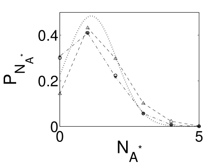
(a) $P(N_{A^{*}})$ at $t=30$

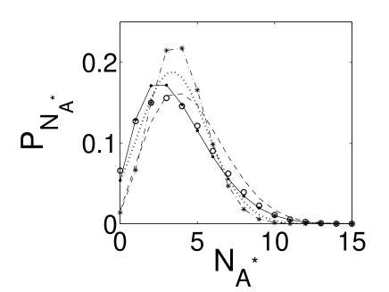
(b) $P(N_{A^{*}})$ at $t=30$

Figure 2: Comparison of the computed distributions for $N_{A^{*}}$ at $t=30$ for the 2-step cascade: Gillespie simulation (circles), one-term basis (dashdotted line), integral form basis (solid line), $\Omega$-expansion (dotted line), Langevin equation (dashed line). (a) $g=10\,,k=5\,,\mu=0.02\,,\lambda=0.15$ with initial condition $(N_{R},N_{R^{*}},N_{A},N_{A^{*}})=(20,0,5,0)$ and (b) $g=0.2\,,k=0.1\,,\mu=0.02\,,\lambda=0.15$, with $(N_{R},N_{R^{*}},N_{A},N_{A^{*}})=(20,0,20,0)$.

For other parameter values, as long as the $R-R^{*}$ reaction is fast, the ansatz Eq. (18) works fine as expected lan1cas . However, if the first reaction is considerably slower than the second one, this ansatz becomes less useful, as shown in Fig. 2(b) for $g=0.2\,,k=0.1\,,\mu=0.02\,,\lambda=0.15$, with $(N_{R},N_{R^{*}},N_{A},N_{A^{*}})=(20,0,20,0)$. The variational result gives a too narrow distribution. The Langevin equation is still not accurate on the left boundary, the average being shifted to the right.

In general, the ansatz (18) tends to generate a distribution narrower than the exact one, which is also shown in Fig. 4(b). This can be explained as follows. The ansatz (18) is a product of functions of $x$ and $y$ and hence only the average particle number $f_{1}$ appears in the second equation of (19). Therefore, the fluctuation generated in the $R-R^{*}$ reaction is absent in the treatment of the $A-A^{*}$ reaction. Physically, if the first reaction is fast, then the second reaction only “sees” an average number of $R^{*}$, with its fluctuation averaged out, and the ansatz (18) produces accurate results (Fig. 2(a)). If the first reaction is slow, however, then the fluctuations in the number of $R^{*}$ strongly influences the $A-A^{*}$ reaction and the mere average $f_{1}$ is not capable of passing this information. The distribution computed from ansatz (18) only accounts for the internal fluctuation of $A-A^{*}$ reaction and hence has a narrower profile than the exact result. On the other hand, despite the apparent simplicity, this ansatz allows one to estimate fluctuations in a reaction network in a semiquantitative way, with an extremely low computational cost, similar to solving the ordinary deterministic kinetics equations.

(a) $P(N_{A^{*}})$ at $t=6$

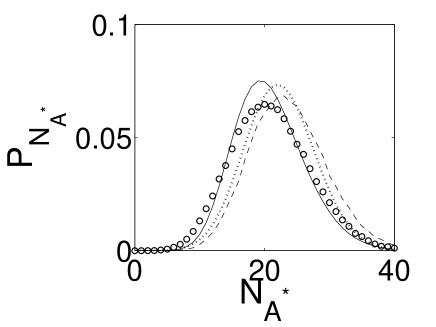
(b) $P(N_{A^{*}})$ at $t=30$

Figure 3: Comparison of the computed distributions for $N_{A^{*}}$ at $t=6$ and $t=30$ for the 2-step cascade: Gillespie simulation (circles), integral form basis (solid line), $\Omega$-expansion (dotted line) and Langevin equation (dashed line). $g=2\,,k=1\,,\mu=0.02\,,\lambda=0.15$ with initial condition $(N_{R},N_{R^{*}},N_{A},N_{A^{*}})=(20,0,100,0)$.

It is straightforward to generalize ansatz (18) to longer cascades. For example, for the 3-step cascades considered next, we may write the right ansatz as

$$\Phi_{R}=(1+f_{3}(t)(z-1))^{N_{2}}(1+f_{2}(t)(y-1))^{N}e^{f_{1}(t)(x-1)}\,.$$ (20)

The resulting ODEs for $f_{i}(t)$’s are similar to Eq. (19) and have a physical interpretation related to the chemical kinetics equations, as discussed above.

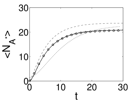
(a) The average

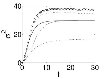
(b) The variance

Figure 4: Comparison of the $N_{A^{*}}$ average and variance computed for the 2-step cascade in time interval $t=[0,30]$: Gillespie simulation (circles), one-term basis (dashdotted line), integral form basis (solid line), $\Omega$-expansion (dotted line) and Langevin equation (dashed line). $g=2\,,k=1\,,\mu=0.02\,,\lambda=0.15$ with initial condition $(N_{R},N_{R^{*}},N_{A},N_{A^{*}})=(20,0,100,0)$.

To get more accurate result, we have to convolute the number fluctuation of $R^{*}$ with the number fluctuation of $A$. Since the ansatz based on simple separation of variables does not work, we need an equation in which $x\,,y$ are explicitly entangled. To facilitate the computation, we use the following integral form representation:

$$\Phi_{R}(x,y)=\int_{-\infty}^{\infty}ds\frac{e^{-s^{2}}}{\sqrt{\pi}}\left(1+f_{2}(t)e^{-(s-f_{3}(t))^{2}}(y-1)+f_{1}(t)(x-1)\right)^{N}\,,$$ (21)

where $f_{1}(t)$ is related to the $R-R^{*}$ reaction and $f_{2}(t)\,,f_{3}(t)$ are related to the $A-A^{*}$ reaction. Note that $\Phi_{R}(1,1)=1$. For $y=1$, we get the expected generating function for $R^{*}$

$$\Phi_{R}(x,1)=\left(1+f_{1}(t)(x-1)\right)^{N}\approx e^{Nf_{1}(t)(x-1)}\,,$$ (22)

the above approximation being valid when $f_{1}(t)$ is small, which is true in all simulations below. We could have used

$$\frac{e^{-s^{2}}}{\sqrt{\pi}}\left(1+f_{2}(t)e^{-(s-f_{3}(t))^{2}}(y-1)\right)^{N}\exp((s-f_{1}(t))^{2}(x-1))$$

in the integrand of (21) to achieve a larger range of $f_{1}$. But when the number of $R^{*}$ is small, ansatz (21) produces better results, probably due to its more convoluted form.

Now we can control both the average and the variance of $A$ by manipulating $f_{2}(t)$ and $f_{3}(t)$. Roughly speaking, $f_{2}(t)$ controls the average and $f_{3}(t)$ controls the variance. For the same parameter set shown in Fig. 2(b), we did the computation by using ansatz Eq. (21) and displayed the result in the same figure (solid line). It matches closely with the exact result, better than all other computations.

To show the effectiveness of the ansatz (21), we use it to do one more computation with $g=2\,,k=1\,,\mu=0.02\,,\lambda=0.15$ and the initial condition $(N_{R},N_{R^{*}},N_{A},N_{A^{*}})=(20,0,100,0)$. In Fig. 3, the distributions of $A^{*}$ are displayed at $t=6$ and $t=30$. Although, the result from ansatz (21) is slightly narrower than the Gillespie computation, they match very well both at $t=6$ and at $t=30$. Actually, this is true for all times as can be seen in Fig. 4 where the time evolution of the average and the variance are depicted. In Fig. 3 and 4, the average of $A^{*}$ from Langevin equation is always greater than the exact result as explained before, although the variance is computed accurately. Curiously, the average from $\Omega$-expansion is smaller initially but later grows larger than the exact one. We also plotted the computation results from Eq. (18). It gives a smaller variance even though the average is quite accurate. In this case, the $R^{*}$ fluctuation is important.

III.3 Application to a three-step amplification cascade

It is not hard to write ansätze similar to Eq. (21) for longer or more complicated cascades. In this section, we demonstrate the use of the variational method for a 3-step cascade with and without feedback loop. In the next section, we will write the equation for a 4-step cascade.

Assume that $A^{*}$ catalyzes a subsequent enzyme activation/deactivation reaction $B\rightleftharpoons B^{*}$ with a forward rate $\mu_{2}$ and a backward decay rate $\lambda_{2}$. The total number $N_{2}$ of $B$ and $B^{*}$ is a constant during the reaction. Following similar procedures as before, we found that the generating function $\Psi(x,y,z)$ satisfies

$$\frac{\partial\Psi}{\partial t} = (1-z)(-\mu_{2}y\frac{\partial^{2}}{\partial y\partial z}-\lambda_{2}N_{2}+(\lambda_{2}z+\mu_{2}*N)\frac{\partial}{\partial z})\Psi$$ (23)

$$+ (1-y)(\mu x\frac{\partial^{2}}{\partial x\partial y}-\lambda N+\lambda y\frac{\partial}{\partial y})\Psi+g(x-1)\Psi-k(x-1)\frac{\partial\Psi}{\partial x}\,,$$

where the first term describes the $B-B^{*}$ reaction. The ansatz similar to Eq. (21) reads

$$\Phi_{R}(x,y,z)=\int_{-\infty}^{\infty}ds\frac{e^{-s^{2}}}{\sqrt{\pi}}\left(1+f_{4}(t)e^{-(s-f_{5}(t))^{2}}(z-1)\right)^{N_{2}}\left(1+f_{2}(t)e^{-(s-f_{3}(t))^{2}}(y-1)+f_{1}(t)(x-1)\right)^{N}\,,$$ (24)

where $f_{4}(t),f_{5}(t)$ describes the $B-B^{*}$ reaction. The calculation results from this ansatz are shown in Fig. 5(a), 6(a) and 7(a).

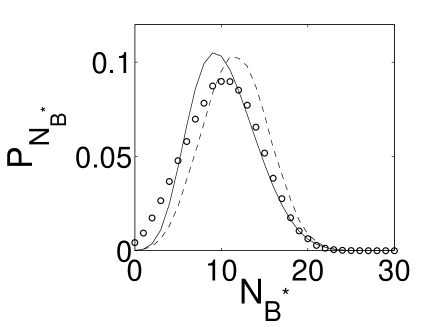
(a) without feedback

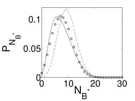
(b) with feedback

Figure 5: Comparison of the computed distributions for $N_{B^{*}}$ at $t=60$ for the 3-step cascade without (a) and with (b) negative feedback: Gillespie simulation (circles), integral form basis (solid line), Langevin equation (dashed line). $g=0.2\,,k=0.1\,,\mu=0.02\,,\lambda=0.15\,,\mu_{2}=0.01\,,\lambda_{2}=0.07\,,\mu_{3}=0.01$ with initial conditions $(N_{R},N_{R^{*}},N_{A},N_{A^{*}},N_{B},N_{B^{*}})=(20,0,20,0,30,0)$.

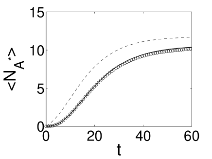
(a) Without feedback

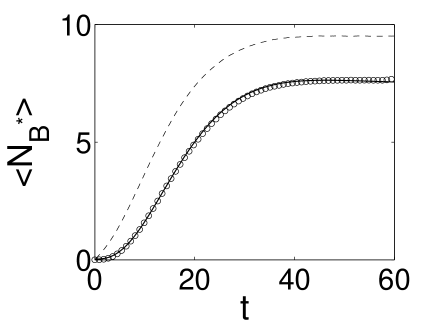
(b) With feedback

Figure 6: Comparison of the $N_{B^{*}}$ average computed for the 3-step cascade without (a) and with (b) negative feedback in time interval $t=[0,60]$: Gillespie simulation (circles), integral form basis (solid line), Langevin equation (dashed line). $g=0.2\,,k=0.1\,,\mu=0.02\,,\lambda=0.15\,,\mu_{2}=0.01\,,\lambda_{2}=0.07\,,\mu_{3}=0.01$ with initial condition $(N_{R},N_{R^{*}},N_{A},N_{A^{*}},N_{B},N_{B^{*}})=(20,0,20,0,30,0)$.

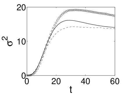
(a) Without feedback

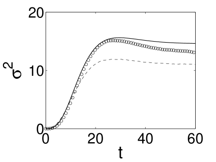
(b) With feedback

Figure 7: Comparison of the $N_{B^{*}}$ variance computed for the 3-step cascade without (a) and with (b) negative feedback in time interval $t=[0,60]$: Gillespie simulation (circles), integral form basis (solid line), Langevin equation (dashed line). $g=0.2\,,k=0.1\,,\mu=0.02\,,\lambda=0.15\,,\mu_{2}=0.01\,,\lambda_{2}=0.07\,,\mu_{3}=0.01$ with initial condition $(N_{R},N_{R^{*}},N_{A},N_{A^{*}},N_{B},N_{B^{*}})=(20,0,20,0,30,0)$.

Shown in Fig. 5(a) is the $B^{*}$ distribution computed from different methods. Ansatz (24) computation matches very well with the exact solution while the Langevin profile is shifted to the right. On the left boundary, both ansatz (24) and Langevin equation approach zero while the exact solution has a finite value there. Interestingly, the variance shows a maximum value during the evolution as displayed in Fig. 7(a). The computation from ansatz (24) captures this non-monotonous behavior accurately which is not obvious at all in the Langevin computation.

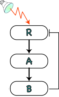
Figure 8: An inactive receptor $R$, when activated by a signal, activates downstream protein $A$, which in turn activates protein $B$. In a negative feedback loop, $B$ downregulates the $R$ activation.

Next, we consider a 3-step signaling cascade with a feedback loop. For example, we can imagine a reaction in which $B^{*}$ turns off the $R^{*}$ signaling, by catalyzing the $R^{*}\to R$ decay at a rate $\mu_{3}$ (Fig. 8). Mathematically, this corresponds to adding an extra term

$$\mu_{3}(1-y)(N_{2}\partial\Psi/\partial x-z\partial^{2}\Psi/\partial x\partial z)$$

to the right hand side of PDE (23). We may still use the same right ansatz (24) and the results are displayed in Fig. 5(b), 6(b) and 7(b). Surprisingly, despite the time scale mixing and nonlinearity, the variational computation matches even better with the exact result than without feedback (compare 5 (a) and (b)). The relative shift of the average computed from the Langevin equation increases. The maximum in the variance still exists but its height decreases with the variance itself. In this case, it seems that the negative feedback sharpens the signal.

III.4 Application to a four-step amplification cascade

Our last demonstration of the variational method is concerned with a 4-step cascade. We append a further enzymatic reaction $C\rightleftharpoons C^{*}$ to our 3-step cascade without feedback. In this reaction, the protein $C$ is switched on with a rate $\mu_{3}$ by $B^{*}$ and decays at a rate $\lambda_{3}$. Again, the total number $N_{3}$ of $C$ and $C^{*}$ is a constant during the reaction. Routinely, we add the corresponding extra term

$$(1-w)(-\mu_{3}z\frac{\partial^{2}}{\partial z\partial w}-\lambda_{3}N_{3}+(\lambda_{3}w+\mu_{3}N_{2})\frac{\partial}{\partial w})\Psi$$

to the right hand side of Eq. (23). The right ansatz is also postulated following the previous pattern,

$$\Phi_{R}(x,y,z,w) = \int_{-\infty}^{\infty}ds\frac{e^{-s^{2}}}{\sqrt{\pi}}\left(1+f_{6}(t)e^{-(s-f_{7}(t))^{2}}(w-1)\right)^{N_{3}}\left(1+f_{4}(t)e^{-(s-f_{5}(t))^{2}}(z-1)\right)^{N_{2}}$$ (25)

$$\left(1+f_{2}(t)e^{-(s-f_{3}(t))^{2}}(y-1)+f_{1}(t)(x-1)\right)^{N}\,,$$

where $f_{6}(t),f_{7}(t)$ describes the $C-C^{*}$ reaction. The computations for a particular set of parameters were carried out and the results are depicted in Fig. 9 and 10.

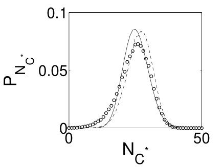
Figure 9: Comparison of the computed distributions for $N_{C^{*}}$ at $t=100$ for the 4-step cascade: Gillespie simulation (circles), integral form basis (solid line) and Langevin equation (dashed line). $g=0.2\,,k=0.1\,,\mu=0.02\,,\lambda=0.15\,,\mu_{2}=0.01\,,\lambda_{2}=0.07\,,\mu_{3}=0.005\,,\lambda_{3}=0.05$ with initial condition $(N_{R},N_{R^{*}},N_{A},N_{A^{*}},N_{B},N_{B^{*}},N_{C},N_{C^{*}})=(20,0,20,0,30,0,50,0)$.

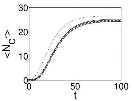
(a) The average

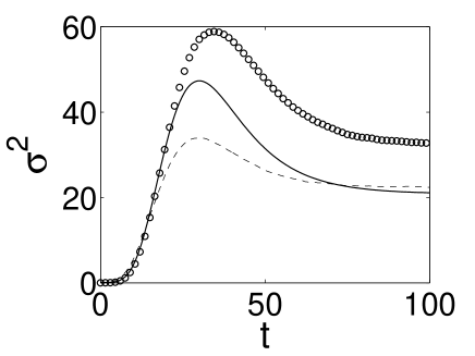
(b) The variance

Figure 10: Comparison of the $N_{C^{*}}$ average and variance computed for the 4-step cascade in time interval $t=[0,100]$: Gillespie simulation (circles), integral form basis (solid line) and Langevin equation (dashed line). $g=0.2\,,k=0.1\,,\mu=0.02\,,\lambda=0.15\,,\mu_{2}=0.01\,,\lambda_{2}=0.07\,,\mu_{3}=0.005\,,\lambda_{3}=0.05$ with initial condition $(N_{R},N_{R^{*}},N_{A},N_{A^{*}},N_{B},N_{B^{*}},N_{C},N_{C^{*}})=(20,0,20,0,30,0,50,0)$.

In Fig. 9, the distributions of $C^{*}$ at $t=100$ from different calculations agree with each other very well. The variational profile is slightly narrower than the exact one but the averages overlap at all times (see Fig. 10(a)). Now, the maximum in the variance becomes more pronounced. Even the Langevin computation clearly displays this feature in Fig. 10(b) though its peak is considerably smaller than the exact one.

IV The advantages and drawbacks of the variational principle

The enzymatic reaction cascades of various lengths considered in section III are a common occurrence, for instance, in the MAPK family of signaling cascades fer97mech ; ch96ul ; bur97mek ; seg95map . It is straightforward to extend the use of our variational scheme to more complex cases, to cascades or networks with complex topology. In general, the generating function is to be postulated in an integral form, as demonstrated earlier for the 2-, 3-, and 4-step cascades, with the time-dependent parameter functions being determined by a set of ODEs derived from the variational principle. Our scheme may be used to treat both the small and large particle number systems. It is many orders of magnitude computationally more efficient in computing the distributions compared with alternative numerical simulation techniques such as the Gillespie algorithm or Langevin equation.

However, in the current form, the ansatz has a number of practical limitations, discussed next. It is difficult to represent efficiently distributions with multiple peaks, for example, or to directly compute transition rates between two deterministically stable states, a common scenario in a gene switch modeling. Another problem is that the derived set of ODEs is quite complicated, thus, symbolic algebra software is necessary to carry out the necessary manipulations. The method accuracy may also depend on the choice of the left ansatz. We chose the current left ansatz form from several trials for simplicity and efficiency. Sometimes when Eq. 12, the time evolution of the unknown functions may result in a possible singularity, requiring workarounds. For reaction types other than the enzymatic one discussed here, such as the binding reactions, the current basis functions may not work properly, since the total particle number of one species (including both the activated and inactive ones) is required to be constant. This may not be true for some arbitrary reaction, necessitating development of new basis functions. However, this is straightforward, and the general principles and considerations that were discussed are expected to apply to those cases as well.

In general, sufficient accuracy may be achieved with a large number of basis functions. The probability distributions are obtained when $\Phi_{R}$ is expanded at $x=0$ and the moments are obtained when $\Phi_{R}$ expanded at $x=1$. Therefore, $\Psi$ together with its derivatives is to be well approximated in the whole interval $x\in[0,1]$. However, the variation equations (11) only consider the validity of Eq. (2) in the neighborhood of $x=1$. It is difficult to estimate the error bounds of $\Psi$ and especially its derivatives near $x=0$, though we know that it generally decreases with increasing accuracy at $x=1$. The choice of basis function, therefore, is essential for the variational technique to be successful.

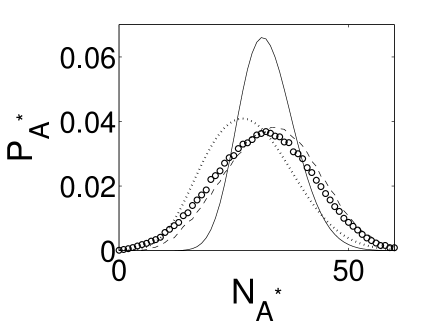
(a) $P(N_{A^{*}})$ at $t=30$

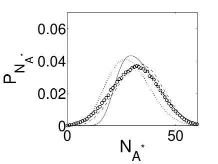
(b) $P(N_{A^{*}})$ at $t=30$

Figure 11: Comparison of the computed distributions for $N_{A^{*}}$ at $t=30$ for the 2-step cascade: Gillespie simulation (circles), integral form basis (solid line), $\Omega$-expansion (dotted line) and Langevin equation (dashed line). $g=0.4\,,k=0.1\,,\mu=0.02\,,\lambda=0.15$ with initial condition $(N_{R},N_{R^{*}},N_{A},N_{A^{*}})=(20,0,100,0)$. (a)$f_{2}(t=30)=0.7304\,,f_{3}(t=30)=0.1413$ calculated by integration of Eq. 19, (b)$f_{2}(t=30)=0.78\,,f_{3}(t=30)=0.3$ estimated by best fitting the exact solution. Shown in the picture is only the distribution profile on $[0,60]$ with other part close to zero.

From the above considerations one may expect that the variational principle itself may still be improved. In Fig. 11, we show the distributions of $A^{*}$ calculated with different methods with a parameter set $g=0.4\,,k=0.1\,,\mu=0.02\,,\lambda=0.15$ and initial conditions $(N_{R},N_{R^{*}},N_{A},N_{A^{*}})=(20,0,100,0)$. In this case, the $R-R^{*}$ reaction is unusually slow compared with the $A-A^{*}$ reaction so that the large fluctuations in the first reaction are retained in the second one. To obtain a highly accurate solution in this parameter regime, a special convolution form was used to solve the generating function PDE in our previous worklan1cas . The current variational scheme, however, underestimates the $A^{*}$ distribution variance. By manually adjusting the $f_{2}\,,f_{3}$, we may obtain a much better fit (solid line in Fig. 11(b)), demonstrating that the variational calculation does not necessarily provide an optimal solution. However, these results suggest that the present time-dependent basis sets are powerful enough to account for these extremely broad distributions. From the experience of numerical solution of ODEs and the conventional variational method in quantum mechanics, a better variational strategy may be to consider simultaneously the validity of Eq. (2) at all points on the interval $[0,1]$. We are currently developing an improved variational approach to address some of the shortcomings discussed above.

V Summary

Cells live in a fluctuating environment in which signals and noise keep bombarding the cell receptors st02gomp ; bar98bac ; sm05inf . Noisy signals propagate inside the cell via microscopic chemical reaction events. Cells have evolved to adapt to or even exploit the seemingly deleterious effect of fluctuations on signaling dynamics within a mesoscopic size object. Thus, it is important to develop a qualitative picture, based on mathematical modeling of stochastic chemical kinetics, of how signaling networks process noisy signals. In this paper, we applied a variational principle to the solution of the master equation which describes the noisy signal propagation.

The essential difficulty associated with the master equation approach is the enormous number of ODEs involved. To compactly encode information, we use a QFT formulation in which the evolution of probability distributions is governed by one “quantum” wave equation. We have explicitly demonstrated the equivalence of the field theoretic formalism with the generating function approach, greatly facilitating the practical application of the variational technique proposed by Eyink eyink96act . We further examined the significance of the variational principle in this context. According to our previous investigation lan1cas , we suggest two novel classes of time-dependent basis functions: one is in simple algebraic form and another is in an integral convolution. These basis functions are key to the successful application of the variational method to various signaling pathways. We applied the new basis functions to describe stochastic signaling in 2-step, 3-step and 4-step enzymatic cascades and compared the obtained results with alternative solution techniques. The variational scheme presented here works favorably in a large parameter range. It treats effectively both the small and the large particle numbers, and is orders of magnitude faster to compute compared with various Monte Carlo simulation algorithms.

However, the current scheme has also some limitations. The resulting evolution equations may be complicated and their derivation requires considerable symbolic manipulation, somewhat ameliorated by using modern computer algebra software. We also showed that the variational principle itself in this context is not the most optimal. Despite these shortcomings, the present variational approach may already be profitably applied to various signal transduction pathways, allowing one to obtain quantitative and semiquantitative solution to stochastic signaling dynamics in a broad range of parameters. The technique may be further improved to extend its limits of applicability, which is a work in progress.

References

- (1) B. D. Gomperts, I. M. Kramer, and P. E. R. Tatham, Signal Transduction, Academic Press, San Diego, 2002.
- (2) D. Bray, Nature 376, 307 (1995).
- (3) B. A. et al, Molecular Biology of the Cell, Garland Science, New York, 2002, Fourth Edition.
- (4) J. Paulsson, O. G. Berg, and M. Ehrenberg, Proc. Natl. Acad. Sci. USA 97, 7148 (2000).
- (5) T. C. Meng, S. Somani, and P. Dhar, In Silico Bio. 4, 0024 (2004).
- (6) T. Shibata and K. Fujimoto, Proc. Natl. Acad. Sci. USA 102, 331 (2005).
- (7) N. Barkai and S. Leibler, Nature 403, 267 (1999).
- (8) K. Wiesenfeld and F. Moss, Nature 373, 33 (1995).
- (9) M. B. Elowitz, A. J. Levine, E. D. Siggia, and P. S. Swain, Nature 297, 1183 (2002).
- (10) P. S. Swain, M. B. Elowitz, and E. D. Siggia, Proc. Natl. Acad. Sci. 99, 12795 (2002).
- (11) E. M. Ozbudak, M. Thattai, I. Kurtser, A. D. Grossman, and A. van Oudenaarden, Nature Genet. 31, 69 (2002).
- (12) W. J. Blake, M. Kaern, C. R. Cantor, and J. J. Collins, Nature 422, 633 (2003).
- (13) L. S. Weinberger, J. C. Burnett, J. E. Toettcher, A. P. Arkin, and D. V. Schaffer, Cell 122, 169 (2005).
- (14) M. Thattai and A. van Oudenaarden, Genetics 167, 523 (2004).
- (15) C. V. Rao, D. M. Wolf, and A. P. Arkin, Nature 420, 231 (2002).
- (16) D. Hansel and G.Mato, Phys. Rev. Lett. 86, 4175 (2001).
- (17) N. I. Markevich, J. B. Hoek, and B. N. Kholodenko, J. Cell Bio. 164, 353 (2004).
- (18) K. C. Huang, Y. Meir, and N. S. Wingreen, Proc. Natl. Acad. Sci. USA 100, 12724 (2003).
- (19) E. Cohen, D. A. Kesseler, and H. levine, Phys. Rev. Lett. 94, 158302 (2005).
- (20) J. P. Keener, Bull. Math. Biol. 63, 625 (2001).
- (21) C. Lemerle, B. D. Ventura, and L. Serrano, FEBS Lett. 579, 1789 (2005).
- (22) R. V. Kulkarni, K. C. Huang, M. Kloster, and N. S. Wingreen, Phys. Rev. Lett. 93, 228103 (2004).
- (23) R. Heinrich, B. G. Neel, and T. A. Rapoport, Molecular Cell 9, 957 (2002).
- (24) M. Chaves, E. D. Sontag, and R. J. Dinerstein, J. Phys. Chem. B 108, 15311 (2004).
- (25) J. P. Keener, J. Theor. Biol. 234, 263 (2005).
- (26) M. Thattai and A. van Oudenaarden, Proc. Natl. Acad. Sci. 98, 8614 (2001).
- (27) A. M. Kierzek, J. Zaim, and P. Zielenkiewicz, J. Biol. Chem. 276, 8165 (2001).
- (28) T. B. Kepler and T. C. Elston, Biophys. J. 81, 3116 (2001).
- (29) M. Sasai and P. G. Wolynes, Proc. Natl. Acad. Sci. USA 100, 2374 (2003).
- (30) A. M. Walczak, M. Sasai, and P. G. Wolynes, Biophys. J. 88, 828 (2005).
- (31) J. R. Pirone and T. C. Elston, J. Theor. Biol. 226, 111 (2004).
- (32) M. Thattai and A. van Oudenaarden, Biophys. J. 82, 2943 (2002).
- (33) P. S. Swain, J. Mol. Biol. 344, 965 (2004).
- (34) N. G. van Kampen, Stochastic processes in physics and chemistry, North Holland Personal Library, Amsterdam, 1992.
- (35) R. F. Fox, Phys. Rev. A 33, 467 (1986).
- (36) D. Holcman and Z. Schuss, J. Chem. Phys. 122, 114710 (2005).
- (37) H. Kuthan, Prog. Biophys. Mol. Biol. 75, 1 (2001).
- (38) S. Y. Shvartsman, C. B. Muratov, and D. A. Lauffenburger, Development 129, 2577 (2002).
- (39) Y. Kuramoto, Prog. Theor. Phys. 52, 711 (1974).
- (40) Y. Lan and G. Papoian, J. Chem. Phys., submitted, (2006).
- (41) N. Yakoby et al., IEE Proc.-Syst. Biol. 152, 276 (2005).
- (42) D. T. Gillespie, J. Phys. Chem. 81, 2340 (1977).
- (43) D. T. Gillespie, J. Chem. Phys. 115, 1716 (2001).
- (44) J. S. van Zon and P. R. ten Wolde, Phys. Rev. Lett. 94, 128103 (2005).
- (45) W. E, D. Liu, and E. Vanden-Eijnden, J. Chem. Phys. 123, 194107 (2005).
- (46) C. W. Gardiner, Handbook of stochastic methods, Springer, New York, 2002.
- (47) M. Doi, J. Phys. A 9, 1479 (1976).
- (48) L. Onsager and S. Machlup, Phys. Rev. 91, 1505 (1953).
- (49) D. C. Mattis and M. L. Glasser, Rev. Mod. Phys. 70, 979 (1998).
- (50) J. Z. Justin, Quantum field theory and critical phenomena, Clarendon Press, Oxford, 2002.
- (51) M. Doi, J. Phys. A 9, 1465 (1976).
- (52) Y. B. Zel’dovich and A. A. Ovchinnikov, Sov. Phys. JETP 47, 829 (1977).
- (53) G. L. Eyink, Phys. Rev. E 54, 3419 (1996).
- (54) F. J. Alexander and G. L. Eyink, Phys. Rev. Lett. 78, 1 (1997).
- (55) J. E. N. Pugh and T. D. Lamb, Biochim. Biophys. Acta 1141, 111 (1993).
- (56) B. Schoeberl, C. Eichler-Jonsson, E. D. Gilles, and G. Müler, Nat. Biotechnol. 20, 370 (2002).
- (57) J. Wang and P. Wolynes, Chem. Phys. 180, 141 (1994).
- (58) N. M. Shnerb, E. Bettelheim, Y. Louzoun, O. Agam, and S. Solomon, Phys. Rev. E 63, 021103 (2001).
- (59) S. Krishnamurthy, E. Smith, D. Krakauer, and W. Fontana, arXiv q-bio.MN, 0312020 (2003).
- (60) O. G. Berg, J. Paulsson, and M. Ehrenberg, Biophys. J. 79, 2944 (2000).
- (61) W. H. Press, S. A. Teukolsky, W. T. Vetterling, and B. P. Flannery, Numerical Recipes in C, Cambridge University Press, Cambridge, England, 1992.
- (62) G. Golub and C. van Loan, Matrix Computations, Johns Hopkins University Press, Baltimore, Maryland, 1996.
- (63) J. Elf and M. Ehrenberg, Genome Research 13, 2475 (2003).
- (64) F. Hayot and C. Jayaprakash, Phys. Bio. 1, 205 (2004).
- (65) Y. Tao, Y. Jia, and T. G. Dewey, J. Chem. Phys. 122, 124108 (2005).
- (66) R. F. Fox and Y. Lu, Phys. Rev. E 49, 3421 (1994).
- (67) J. J. E. Ferrell and R. R. Bhatt, J. Bio. Chem. 272, 19008 (1997).
- (68) C.-Y. F. Huang and J. J. E. Ferrell, Proc. Natl. Acad. Sci. USA 93, 10078 (1996).
- (69) W. R. Burack and T. W. Sturgill, Biochemistry 36, 5929 (1997).
- (70) R. Seger and E. G. Krebs, FASEB J. 99, 726 (1995).
- (71) N. Barkai and S. Leibler, Nature 393, 18 (1998).
- (72) V. N. Smelyankiy, D. G. Luchinsky, A. Stefanovska, and P. V. E. McClintock, Phys. Rev. Lett. 94, 98101 (2005).