Self-wiring in neural nets of point-like cortical neurons fails to reproduce cytoarchitectural differences

Abstract

We propose a model for description of activity-dependent evolution and self-wiring between binary neurons. Specifically, this model can be used for investigation of growth of neuronal connectivity in the developing neocortex. By using computational simulations with appropriate training pattern sequences, we show that long-term memory can be encoded in neuronal connectivity and that the external stimulations form part of the functioning neocortical circuit. It is proposed that such binary neuron representations of point-like cortical neurons fail to reproduce cytoarchitectural differences of the neocortical organization, which has implications for inadequacies of compartmental models.

I Introduction

The nature of processes, underlying the brain’s self-organization into functioning neocortical circuits remains unclear. For theoretical description of activity-independent and activity-dependent emergence of complex spatio-temporal patterns, and establishment of neuronal connections, various methods have been proposed 21 ; 22 ; 23 ; 2 ; 5 ; 49 . These theoretical investigations give a fresh understanding of the observed phenomena and stimulate discovery of emergent features of neural circuits. In this paper, we propose a new theoretical approach for description of activity-dependent evolution and self-wiring between binary neurons. We propose a model based on the following experimental data (1)-(3) and hypotheses (4)-(5):

1. Development of neuronal connectivity dependents on the neurons activity 46 ; 26 ; 36 ; 1 ;

2. Direction of motion of the growth cones is controlled by diffusible chemicals -axon guidance molecules (AGM) 19 ; 8 ; 15 ; 20 ;

3. Axon’s growth rate dependence on the neuron’s activity 29 ; 31 ; 30 ; 28 ;

4. Depolarization causes neurons to release axon guidance 35 ; 34 ;

5. Type of neuronal connectivity is determined postsynaptically during synaptogenesis 33 ; 40 ; 41 .

A state of all cells at some moment we shall call the activity pattern. Sequential alternation of activity patterns we shall call activity dynamics. We suppose that each neuron receives an external signal from a sensory cell (optical, taste, smell, ets.). Patterns of external signals we will call training patterns. We demonstrate an example of training process by stimulation of the developing net by the sequence of training patterns. The sequence of training patterns can be considered as a training program. The goal of the training is creation of complex connections structure between initially disconnected neurons. For mathematical description of net’s electrical activity we use the simplest model 50 . We take into account only properties which are most important for description of the activity-dependent self-wiring.

II Mathematical framework

In this section we consider a mathematical basis for description of the activity - dependent self-wiring in neural nets. For mathematical description of neurons states and activity patterns, we use simple representation from modern neurobiology and artificial neural nets (ANN) theory. At state of rest neuronal membrane is polarized. When the membrane is locally depolarized up to the certain value of transmembrane potential by opening the ligand activated synaptic ion channels, then the voltage gated ion channels are opened which causes the generation of the action potential. The action potential travels along the axon and causes local depolarization of another neurons through synapses. We suppose that each cell at each moment of time can be in two states: active, $S_{i}(t_{j})=1$, or inactive, $S_{i}(t_{j})=0$. For real neurons the active state can be regarded as the real neuron’s single spike or a sequence of spikes with frequency above some value.

We consider the $i$-th neuron’s cell body as a spherical object with center at the point with the radius-vector ${\bf r}_{i}$ in extracellular environment. For implementation activity-dependent release of AGM in our model, we suppose that neurons release AGM at a moment of depolarization. For simplification we assume that all neurons fire and release AGM synchronous, depending on their state. AGM which have released by neurons diffuse through the extracellular space, then bind axon’s growth cones receptors and control their growth. When we consider AGM release by neurons, we neglect geometrical properties of them and consider them as a point sources of AGM.

According to our model if the cell is in active state, $S_{i}(t_{k})=1$, it releases some amount of AGM. We suppose that all neurons release the unit amount of the one type AGM which causes only attraction of growth cones.

For description of AGM diffusion process we use a simple diffusion equation. The concentration of AGM, $c_{ij}$, released by the i-th cell at the moment $t_{j}$ can be found as the solution of the equation

$$\frac{\partial c_{ij}}{\partial{t}}=D^{2}\Delta c_{ij}-kc_{ij}$$ (2.1)

with the initial conditions $c_{ij}({\bf r},{\bf r}_{i},t_{j})=\delta({\bf r}-{\bf r}_{i})S_{i}(t_{j})$. Here $D$ and $k$ are AGM diffusion and degradation coefficients in the intracellular medium. We consider here the case without boundary conditions. The solution of this equation, describing the concentration of AGM at the point ${\bf r}$ at the time $t$ is

$$c_{ij}({\bf r},{\bf r}_{i},t,t_{j})=\frac{S_{i}(t_{j})}{(2D\sqrt{\pi(t-t_{j})})^{3}}\exp\left(-k(t-t_{j})-\frac{|{\bf r}-{\bf r}_{i}|^{2}}{4D^{2}(t-t_{j})}\right).$$ (2.2)

Total concentration of AGM at the point $\mathbf{r}$ can be found by summation of concentrations of AGM which were released by each cell

$$C({\bf r},t)=\sum_{i=1}^{N}\sum_{j=1}^{k}c_{ij}({\bf r},{\bf r}_{i},t,t_{j}).$$ (2.3)

According to the experimental data we suppose that a growth cone will move only if its soma is at inactive state, and the force acting on it is proportional to AGM concentration gradient $\nabla C$ at the growth cone’s position. Therefore, the equation of motion of the $n$-th neuron’s $k$-th growth cone, described by the radius-vector ${\bf g}_{k}^{n}$ in the chemical field can be written in the following form

$$\frac{d{\bf g}_{k}^{n}}{dt}=\lambda\nabla C({\bf g}_{k}^{n},t)[S_{n}(t)-1].$$ (2.4)

Here $\lambda$ is a coefficient describing axon’s sensitivity and motility. Taking into account the expression for total concentration from Eqn. 2.3 and using it into Eqn. 2.5 we obtain

$$\frac{d{\bf g}_{k}^{n}}{dt}=\lambda[S_{n}(t)-1]\sum_{i=1}^{N}\sum_{j=1}^{k}\nabla c_{ij}({\bf g}_{k}^{n},{\bf r}_{i},t,t_{j}).$$ (2.5)

From Eq. 2.2 we find the expression for gradient of AGM concentration $c_{ij}$ in the form below

$$\nabla c_{i,j}({\bf r},{\bf r}_{i},t,t_{i})=-\frac{S_{i}(t_{j})({\bf r}-{\bf r}_{i})}{16D^{5}\pi^{\frac{3}{2}}(t-t_{j})^{\frac{5}{2}}}\exp\left(-k(t-t_{j})-\frac{|{\bf r}-{\bf r}_{i}|^{2}}{4D^{2}(t-t_{j})}\right).$$ (2.6)

If a some growth cone is close to the another cell’s soma, i.e if $|{\bf g}_{k}^{n}-{\bf r}_{i}|<\varepsilon$ ($\varepsilon$ can be considered as the soma’s geometrical radius) then synaptogenesis process takes place, and synaptic connection between these neurons will be established. Type of the neuronal connections between $i$-th and $n$-th neurons we describe by using synaptic weights $w_{n,i}$ ($w_{n,i}=1$ means excitatory and $w_{n,i}=-1$ inhibitory connections). In our model the type of synaptic connection established between neurons depends on the state of postsynaptic cell at synaptogenesis moment (if $S_{i}(t_{k})=1$ then $w_{n,i}=1$, else $w_{n,i}=-1$).

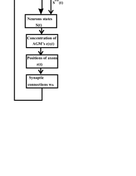
Figure 1: A flowchart of self-wiring process

For implementation network’s electrical activity dynamics several models can be used (firing rate models, integrate and fire neurons, etc.). For simplicity we will exploit the simplest one. We assume that the state of each cell at next moment of time is determined by states of another neuron, and neuronal connections weights, and external signal. Each postsynaptic cell integrates inputs coming from all presynaptic neuron and an external signal $S_{i}^{ext}$

$$s=\sum_{n=1}^{N}w_{n,i}S_{n}(t_{i})+S_{i}^{ext},$$ (2.7)

and the state of each neuron at next moment is determined by following rule: if $s>0$ then $S_{i}(t_{i+1})=1$, else $S_{i}(t_{i+1})=0$.

This model gives a closed set of equations describing AGM’s release and diffusion, and axons grow and neuronal connections establishment as well as the net’s electrical activity dynamics. In the flowchart (Fig. 1) the back loop in the neural net’s activity-dependent development and self-wiring are shown. The concentration of AGM in the extracellular space is controlled by neurons state. Growth and movement of growth cones is managed by the concentration gradients of AGM. Growth cones can make neuronal connections with other neurons and change the network’s connections structure which change the network’s activity.

III Numerical analysis

In this section we present the result of the numerical simulation of the self-wiring net presented above. For testing possibilities and properties of self-wiring nets we use the net with $27$ neurons, $N=27$, placed at the points with radius-vectors ${\bf r_{1}}=(0,0,1)$, ${\bf r}_{2}=(0,0,0)$, ${\bf r}_{3}=(0,-1,0)$, … ${\bf r}_{27}=(1,1,-1)$ (see Fig. 3). Each neuron has $27$ growth cones, which can be considered as branches of its axon. Initially all growth cones are located near the soma ${\bf g}_{k}^{n}={\bf r}_{k}+{\bf\varepsilon}$, $|{\bf\varepsilon}|<0.01$, and all synaptic weights equal to zero ($w_{ik}=0$ $i,j=1...N$).

We can write the Eqn. 2.6 for AGM’s gradient using a discrete time $t=n\Delta t$ (present time), $t_{m}=m\Delta t$ (release time) in the following form

$$\nabla c({\bf r},{\bf r}_{i},m\Delta t,n\Delta t)=\frac{S_{i}(n\Delta t)({\bf r}-{\bf r}_{i})}{16D^{5}\pi^{\frac{3}{2}}((n-m)\Delta t)^{\frac{5}{2}}}\exp\left(-kt-\frac{|{\bf r}-{\bf r}_{i}|^{2}}{4D^{2}(n-m)\Delta t}\right),$$ (3.8)

where $\Delta t$ is a time interval between the net’s iterations. For simplification we set $\Delta t=1$ and rewrite the Eqn. 3.8 in terms of indices $m$, $n$

$$\nabla c_{m,n}({\bf r},{\bf r}_{i})=\frac{S_{i}(n)({\bf r}-{\bf r}_{i})}{16D^{5}\pi^{\frac{3}{2}}(n-m)^{\frac{5}{2}}}\exp\left(-kt-\frac{|{\bf r}-{\bf r}_{i}|^{2}}{4D^{2}(n-m)}\right).$$ (3.9)

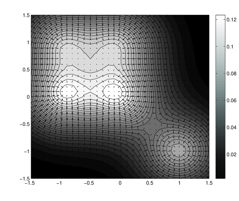
Figure 2: The contour plot of target-derived AGM concentration. The concentration of AGM is higher in lighter regions of the figure. The arrows reproduce the concentration gradients which means the axons movement directions for the particular place.

For numerical integration a growth cone equation of motion 2.5 we have to rewrite it in terms of the discrete time. Using the time interval $\Delta t=1$ we obtain the recursion relation which allow us calculate the spatial position of each growth cone at the moment $k+1$ in terms of the $k$-th moment

$${\bf g}_{k+1}={\bf g}_{k}+\lambda[S_{n}(t_{k})-1]\sum_{i=1}^{N}\sum_{m=1}^{k}\nabla c_{m,k}({\bf g_{k}},{\bf r}_{i}).$$ (3.10)

In above equation we have omitted indices, describing a cell’s and the growth cone’s number. The value $\Delta t=1$ is not critical for numerical calculations of the model and it was used only for simplification point of view. Different values of parameters $D$, $k$, $\lambda$ gives different connectivity patterns between neurons, because these parameters characterize growth cone’s movement speed, and AGM’s acting distance, and etc. Basic properties of the net have remained unchanged. For all subsequent numerical calculations we used the following values: $D=0.1$, $k=0.1$, $\lambda=10$.

In Fig. 2 we present the contour plot of the section by plane $z=0.02$ the static AGM concentration when the $6$-th, $7$-th, $15$-th, $16$-th, $19$-th neurons are in active state. The arrows reproduce the concentration gradients which means the axons movement directions for the particular place.

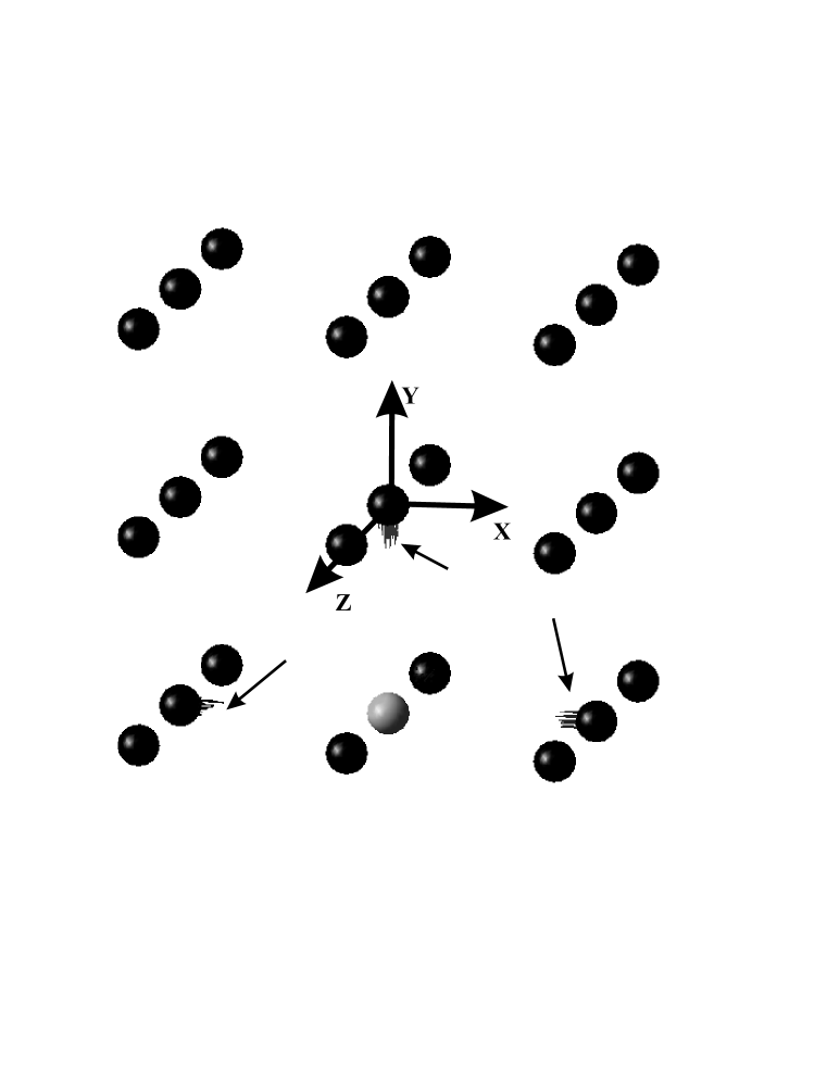
Figure 3: Activity-dependent evolution at the beginning of simulation $(n=110)$, see Section III. One of the cell has stimulated by the external signal $S_{11}^{ext}=1$ (bright sphere), and other neurons are at inactive state. The axon’s branches of the nearest neurons have started to grow in the direction of the active cell because it releases AGM.

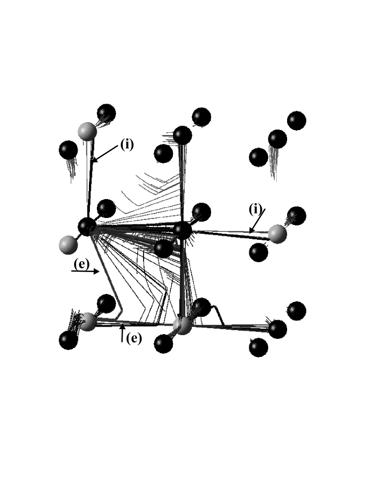
Figure 4: Activity-dependent evolution at $n=680$. Between some of the neurons inhibitory (i) and excitatory (e) connections have been established.

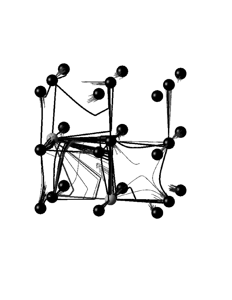
Figure 5: Activity-dependent evolution at $(n=910)$. By using the training program the complicated connections pattern between neurons have been created. The network has following neuronal connections: $w_{10,11}=1$, $w_{12,11}=1$ ,$w_{2,11}=1$, $w_{13,14}=-1$, $w_{15,14}=-1$, $w_{5,14}=-1$, $w_{23,14}=-1$, $w_{17,14}=-1$, $w_{11,14}=1$, $w_{6,5}=-1$, $w_{4,5}=-1$, $w_{8,5}=-1$, $w_{2,5}=1$, $w_{11,5}=-1$, $w_{17,5}=-1$, $w_{15,5}=-1$, $w_{13,5}=-1$, $w_{12,5}=1$, $w_{14,5}=1$, $w_{10,5}=1$, $w_{14,11}=-1$, $w_{20,11}=-1$, $w_{1,2}=-1$, $w_{3,2}=-1$, $w_{7,8}=-1$, $w_{23,24}=-1$, $w_{22,23}=-1$, $w_{26,23}=-1$, $w_{9,6}=-1$, $w_{15,6}=-1$, $w_{9,8}=-1$, $w_{17,8}=-1$, $w_{3,6}=-1$, $w_{12,2}=-1$, $w_{14,2}=-1$, $w_{5,11}=-1$, $w_{5,6}=-1$, $w_{14,23}=-1$, $w_{17,6}=-1$, $w_{12,6}=-1$, $w_{14,6}=-1$, $w_{10,6}=-1$, $w_{20,6}=-1$, $w_{20,2}=-1$, $w_{13,16}=-1$, $w_{20,23}=-1$, $w_{10,2}=-1$, $w_{13,11}=-1$, $w_{5,2}=1$.

By using the appropriate training patterns sequence the net is built with inhibitory and excitatory connections which is evolved in oscillatory manner without any external stimulation. As an example we present the results of the network training process which was obtained by using the following training pattern sequence: $S_{11}^{ext}=1$ for $10<n<192$; $S_{14}^{ext}=1$ for $192<n<360$; $S_{5}^{ext}=1$ for $360<n<515$; $S_{5}^{ext}=1$ for $525<n<576$; $S_{2}^{ext}=1$ for $580<n<875$; $S_{6}^{ext}=1$ for $580<n<880$; $S_{8}^{ext}=1$ for $580<n<880$; $S_{23}^{ext}=1$ for $580<n<880$. In Fig. 3 we reproduce three dimensional picture of the state of the net at the simulation beginning. Individual neurons (whilst without neuronal connections) depicted as spheres and its states depicted by color (bright - active state, dark- inactive). The travelling axon’s branches are depicted as thin curves. One can see from this figure, how axons grow toward the active cell. When the growth cone reaches the soma of another neuron, two neurons became connected and axon’s connected branch is depicted by thick curve (Fig. 4). The synapse type (inhibitory or excitatory) is depicted by color of a curve (bright - excitatory, dark- inhibitory). When the branch of the same axon reaches the another cell, which has already connected with it, this branch will be deleted. The neural net obtained by training is shown in Fig. 5.

Further training of this net is a hard problem because the internal oscillation will influence to the training process. The oscillating patterns of neuronal activity will cause establishment of new connections, even after switching off the external stimulation, and can cause uncontrolled self-wiring. In forthcoming papers we plan to develop programming (training) methods in order to build the net with initially defined connections.

We can gain access to the patterns stored in the net by stimulating them by external patterns. Because of an external stimulation will cause activation of neurons and release of AGM we conclude that access to the memory can change the connectivity pattern, i.e. patterns stored in the memory.

IV Conclusions

In this paper we presented a mathematical model describing processes of self-wiring in neural nets. The model can give us a new understanding of real neural nets development and functioning. By using the computer simulations we showed that the long-time memory can be encoded in neuronal connectivity and in what way the external stimulations builds a functioning neural network.

Hypotheses proposed here should be tested experimentally (in vivo, in vitro), for verification the possibilities of presented model application for qualitative and quantitative description of a neuronal integration processes in a real nets. Our approach gives only general modeling scheme of activity-dependent network formation processes and to accordance with experimental data the model can be complicated and a particular rules describing separate processes can be changed.

The theoretical framework developed here, can be used for description the development of a particular set of neurons constituting the neural system, which can be located in the media containing also another type neurons and glia cells. In our model axon’s branches began to growth directly from the soma. In a real nets growth cones can be guided at the growth beginning by another mechanisms (genetically determine contact adhesion, etc) and then by the mechanism presented in this paper. Geometrical properties and activity of real neurons are more complicate and they have dendrites. Here we used the most simple representations of hypothetical neurons (large spherical soma without dendrites ) and its activity (binary neurons). Using the approach described here it is possible to construct a model for description real particular networks, using more realistic models of neurons (ingrate-and-fire, Hodgkin-Huxley, etc) and taking into account neurons geometrical properties and dendrites. We suppose that the model presented can be used for description self-wiring processes in a developing (embryonal) as well as adult neuronal systems.

Cytoarchitectural differences between different cortical areas are the result of differences in distributions of neuronal phenotypes and morphologies. Self-wiring between binary neurons fails to reproduce cytoarchitectural differences of the neocortical organization, which has implications for inadequacies of compartmental models. In order to reproduce cytoarchitectural differences, axonal and dendritic morphologies of single neurons Kal need to be integrated into the model.

References

- (1) Andras P, A model for emergent complex order in small neural networks, J. Integr. Neurosci. 3:55-69, 2003
- (2) Ascoli GA, Passive dendritic integration heavily affects spiking dynamics of recurrent networks, Neural Netw. 16:657-663,2003.
- (3) Balkoweic A, David MK, Activity-dependent release of endogenous brain-derived neurotrophic factor from primary sensory neurons detected by ELISA in Situ, J. Neurosc. 20:7417-7423, 2000.
- (4) Borodinsky LN, Root CM, Cronin JA, Sann SB, Gu X, Spitzer C, Activity-dependent homeostatic specification of transmitter expression in embrionic neurons, Nature 429:523-530, 2004.
- (5) Catalano SM Shatz CJ, Activity-Dependent Cortical Target Selection by Thalamic Axons, Science 281:559-562, 1998.
- (6) Chauvet GA, On the mathematical integration of the nervous tissue based on the S-propagator formalism I: Theory, J. Integr. Neurosci. 1:31-68, 2002
- (7) Chauvet P, Chauvet GA, On the mathematical integration of the nervous tissue based on the S-propagator formalism II: Numerical simulations for molecular-dependent activity, J. Integr. Neurosci. 1:157-194, 2002.
- (8) Ciccolini F, Collins TJ, Sudhoelter J, Lipp P, Berridge MJ, Local and Global Spontaneous Calcium Events Regulate Neurite Outgrowth and Onset of GABAergic Phenotype during Neural Precursor Differentiation, J. Neurosc. 23:103-111, 2003.
- (9) Dickson BJ, Molecular Mechanisms of Axon Guidance, Science 298:1959-1964, 2002.
- (10) Dugué GP, Dumoulin A, Triller A, Dieudonne S, Target-Dependent Use of Coreleased Inhibitory Transmitters at Central Synapses, J. Neurosc. 25:6490-6498, 2005.
- (11) Goodhill GJ, Gu M, Urbach JS, Predicting axonal response to molecular gradient with a computational model of filopodial dynamics, Neural Comp. 16:2221-2243, 2004.
- (12) Gomez TM, Spitzer NC, Regulation of growth cone behavior by calcium: new dynamics to earlier perspectives, J. Neurobiol, 44:174-183, 2000.
- (13) Gomez TM, Spitzer NC, In vivo regulation of axon extension and pathfinding by growth-cone calcium transients, Nature, 397:35-355, 1999.
- (14) Hartmann M, Heumann R, Lessman V, Synaptic secretion of BDNG after high-frequency stimulation in glutamatergic synapses, The EMBO J. 20:5887-5897, 2001.
- (15) Henley J, Poo MM, Guiding neuronal growth cones using signals, Trends Cell Biol., 14:320-330, 2004.
- (16) Hentschel HGE, van Ooyen A, Models of axon guidance and bunding during development, Proc. R. Soc. Lond B 266:2231-2238, 1999.
- (17) Kalisman N, Silberberg G, Markram H, Deriving physical connectivity from neuronal morphology, Biol. Cybern. 88:210-218, 2003.
- (18) Kandler K, Activity-dependent organization of inhibitory circuits: lessons from the auditory system, Curr. Opin. Neurobiol. 14:96-104, 2004.
- (19) Ming GL, Henley J, Tessier-Lavigne M, Song H.-J, Poo M.-M, Electrical activity modulates growth cone guidance by diffusible factors, Neuron, 29:441-452, 2001.
- (20) Nieto MA, Molecular Biology of Axon Guidance, Neuron 17 :1039-1048, 1996.
- (21) van Ooyen A, van Pelt J, Activity-dependent outgrowth of neurons and overshot phenomena in developing neural networks, J.theor. Biol 167:27-43,1994.
- (22) van Ooyen A, van Pelt J, Complex Periodic Behavior in a neural network model with activity-dependent neurite outgrowth, J. Theor. Biol. 179:229-242, 1996.
- (23) van Pelt J, Kamermans M, Levelt CN, Van Ooyen A, Ramakers GJA, Roelfsema PR (eds.), Development, Dynamics and Pathology of Neuronal Networks: From Molecules to Functional Circuits, Prog. Brain Res. 147, Elsevier, Amsterdam, 2005.
- (24) Segev R, Ben-Jacob E, Generic modeling of chemotactic based self-wiring of neural networks, Neural Networks 13:185-199, 2000.
- (25) Tessier-Lavigne M., Goodman CS, The Molecular Biology of Axon Guidance, Science 274:1123-1133, 1996.