Designing Complex Networks

Abstract

We suggest a new perspective of research towards understanding the relations between structure and dynamics of a complex network: Can we design a network, e.g. by modifying the features of units or interactions, such that it exhibits a desired dynamics? Here we present a case study where we positively answer this question analytically for networks of spiking neural oscillators. First, we present a method of finding the set of all networks (defined by all mutual coupling strengths) that exhibit an arbitrary given periodic pattern of spikes as an invariant solution. In such a pattern all spike times of all the neurons are exactly predefined. The method is very general as it covers networks of different types of neurons, excitatory and inhibitory couplings, interaction delays that may be heterogeneously distributed, and arbitrary network connectivities. Second, we show how to design networks if further restrictions are imposed, for instance by predefining the detailed network connectivity. We illustrate the applicability of the method by examples of Erdös-Rényi and power-law random networks. Third, the method can be used to design networks that optimize network properties. To illustrate the idea, we design networks that exhibit a predefined pattern dynamics and at the same time minimize the networks’ wiring costs.

1 How does network structure relate to dynamics?

Our understanding of complex systems, in particular biological ones, ever more relies on mathematical insights resulting from modeling. Modeling a complex system, however, is a highly non-trivial task, given that many factors such as strong heterogeneities, interaction delays, or hierarchical structure often occur simultaneously and thus complicate mathematical analysis.

Many such systems consist of a large number of units that are at least qualitatively similar. These units typically interact on a network of complicated connectivity. Important example systems range from gene regulatory networks in the cell and networks of neurons in the brain to food webs of species being predator or prey to certain other species [3, 17, 11].

A major question is how the connectivity structure of a network relates to its dynamics and its functional properties. Researchers therefore are currently trying to understand which kinds of dynamics result from specific network connectivities such as lattices and random networks as well as networks with small-world topology or power-law degree distribution. [31, 26, 30]

Here we suggest a complementary approach: network design. Can we modify structural features of a complex network such that it exhibits a desired dynamics? We positively answer this question analytically for a class of spiking neural network models and illustrate our findings by numerical examples.

In neurophysiological experiments, recurring patterns of temporally precise and spatially distributed spiking dynamics have been observed in different neuronal systems in vivo and in vitro [19, 29, 37, 14]. These spike patterns correlate with external stimuli (events) and are thus considered key features of neural information processing [2]. Their dynamical origin, however, is unknown. One possible explanation for their occurrence is the existence of excitatorily coupled feed-forward structures, synfire chains [1, 15, 10, 5], which are embedded in a network of otherwise random connectivity and receive a large number of random external inputs. Such stochastic models explain the recurrence of coordinated spikes but do not account for the specific relative spike times of individual neurons, although these are discussed to be essential for computation, too. To reveal mechanisms underlying specific spike patterns and their computational capabilities, our long term aim is to develop and analyze a new, deterministic network model that explains the occurrence of specific precisely timed spike patterns exhibiting realistic features. The work presented here constitutes one of the first steps in this direction (cf. also [18, 20, 9]) and focuses on designing networks such that they exhibit an arbitrary predefined periodic spike pattern.

The article is organized as follows. In section 2 we introduce a class of network models of spiking neurons and illustrate their relation to standard modeling approaches using differential equations. In section 3 we design networks by deriving systems of equations and inequalities that analytically restrict the set of networks (in the space of all coupling strengths) such that they exhibit an arbitrary predefined periodic spike pattern as an invariant dynamics. It turns out that such systems are often underdetermined such that further requirements on the individual units, the interactions and the network connectivity can be imposed. We illustrate this in section 4 by specifying completely, for each neuron, the sets of other neurons it receives spikes from, i.e. the entire network connectivity. We present examples of networks with specified connectivities of different statistics and design their coupling strengths such that they exhibit the same spike pattern. In section 5 we demonstrate the possibility of designing networks that are optimal (with respect to some cost function). We present illustrating examples of networks that exhibit a certain pattern of precisely timed spikes and at the same time minimize wiring costs. In section 6 we provide a brief step-by-step instruction for applying the presented method. Section 7 provides the conclusions and highlights open questions regarding the design of complex networks.

The method of finding the set of networks exhibiting a predefined pattern (parts of sections 2 and 3 of this article) was briefly reported before in reference [23] and in abstract form in [22], where only the case of non-degenerate patterns, identical delays and identical neurons was treated explicitely. Small inhomogeneities have been discussed in [9]. Here we include also degenerate patterns, heterogeneously distributed delays and allow for different neuron types. Moreover, we present new applications of network design, see in particular sections 4 and 5.

2 Model neural networks

2.1 Phase model

Consider a network of $N$ oscillatory neurons that interact by sending and receiving spikes via directed connections. The network connectivity is arbitrary and defined if we specify for each neuron $l\in\{1,\ldots,N\}$ the sets $\operatorname{Pre}(l)$ from which it receives input connections. One phase-like variable $\phi_{l}(t)$ specifies the state of each neuron $l$ at time $t$. A continuous strictly monotonic increasing rise function $U_{l}$, $U_{l}(0)=0$, defines the membrane potential $U_{l}(\phi_{l})$ of the neuron, representing its subthreshold dynamics [25], see Fig. 1. The neurons interact at discrete event times when they send or receive spikes. We first introduce the model for non-degenerate events, i.e. non-simultaneous event times, and provide additional conventions for degenerate events in the next subsection.

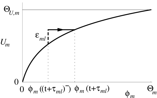
Figure 1: Phase dynamics in response to incoming excitatory spike. The rise function $U_{m}$ of neuron $m$ is plotted as a function of its phase $\phi_{m}$. In the absence of interactions, $\phi_{m}(t)$ increases uniformly with time $t$ according to Eq. (1). If a spike is sent by neuron $l$ at time $t$, it is received by neuron $m$ at time $t+\tau_{ml}$ and induces a phase jump $\phi_{m}((t+\tau_{ml})^{-})\rightarrow\phi_{m}(t+\tau_{ml})$ that is mediated by the rise function $U_{m}$ and its inverse according to (2) and (3). Here $\Theta_{U,m}=U_{m}(\Theta_{m})$ is the threshold for the membrane potential, cf. sec. 2.3.

In the absence of interactions, the phases increase uniformly obeying

$$d\phi_{l}/dt=1.$$ (1)

When $\phi_{l}$ reaches the (phase-)threshold of neuron $l$, $\phi_{l}(t^{-})=\Theta_{l}>0$, it is reset, $\phi_{l}(t)=0$, and a spike is emitted. After a delay time $\tau_{ml}$ this spike signal reaches the post-synaptic neuron $m$, inducing an instantaneous phase jump

$$\phi_{m}\left(t+\tau_{ml}\right)=H_{\varepsilon_{ml}}^{(m)}\left(\phi_{m}\left(\left(t+\tau_{ml}\right)^{-}\right)\right),$$ (2)

mediated by the continuous response function

$$H_{\varepsilon}^{(m)}(\phi)=U_{m}^{-1}(U_{m}(\phi)+\varepsilon)$$ (3)

that is strictly monotonic increasing, both as a function of $\varepsilon$ and of $\phi$. Here, $\varepsilon_{ml}$ denotes the strength of the coupling from neuron $l$ to $m$. This coupling is called inhibitory if $\varepsilon_{ml}<0$ and excitatory if $\varepsilon_{ml}>0$. We note that sending and receiving of spikes are the only nonlinear events occurring in these systems. Throughout the manuscript, $\phi_{l}(t)$ is assumed to be piecewise linear for all $l$ such that in any finite time interval there are only a finite number of spike times.

2.2 Degenerate event timing

These events of sending and receiving spikes might sometimes occur simultaneously such that care has to be taken in the definition of the model dynamics. Simultaneous events occurring at different neurons do not cause any difficulties because an arbitrary order of processing does not affect the collective dynamics at any future time. However, if two or more events occur simultaneously at the same neuron, we need to specify a convention for the order of processing. We will therefore go through the possible combinations in the following:

(i) spike sending due to spike reception: The action of a received spike might be strong enough such that the excitation is supra-threshold,

$$U_{m}\left(\phi_{m}\left(\left(t+\tau_{ml}\right)^{-}\right)\right)+\varepsilon_{ml}\geq U_{m}\left(\Theta_{m}\right).$$ (4)

We use the convention that neuron $m$ sends a spike simultaneous to the reception of another spike from neuron $l$ at time $t+\tau_{ml}$ and is reset to

$$\phi_{m}\left(t+\tau_{ml}\right)=0.$$ (5)

(ii) spike received at sending time: If neuron $m$ receives a spike from neuron $l$ exactly at the same time when $m$ was about to send a spike anyway,

$$\phi_{m}\left(\left(t+\tau_{ml}\right)^{-}\right)=\Theta_{m},$$ (6)

we take the following convention for the order processing: first the spike is sent and the phase is reset to zero, then the spike is received such that

$$\phi_{m}\left(t+\tau_{ml}\right)=H_{\varepsilon_{ml}}^{(m)}\left(0\right).$$ (7)

If the spike received causes again a supra-threshold excitation, we neglect a second spike potentially generated at time $t+\tau_{ml}$ and just reset the neuron $m$ to zero as in (5).

(iii) simultaneous reception of multiple spikes: If multiple spikes are received simultaneously by the same neuron and each subset of spikes does not cause a supra-threshold excitation (as in (4)), a convention about the order of treatment is not necessary as can be seen from the following argument. If neuron $m$ at time $\theta$ simultaneously receives $h\in\mathbb{{N}}$ spikes from neurons $l_{1},...,l_{h\,}$, and $\sigma:\{1,...,h\}\rightarrow\{1,...,h\}$ is an arbitrary permutation of the first $h$ integers, we have

$$H_{\varepsilon_{ml_{\sigma(1)}}}^{(m)}(H_{\varepsilon_{ml_{\sigma(2)}}}^{(m)}(...H_{\varepsilon_{ml_{\sigma(h)}}}^{(m)}(\phi_{m}(\theta^{-}))...))$$

$$= U_{m}^{-1}[U_{m}(U_{m}^{-1}[U_{m}(...U_{m}^{-1}[U_{m}(\phi_{m}(\theta^{-}))+\varepsilon_{ml_{\sigma(h)}}]...)+\varepsilon_{ml_{\sigma(2)}}])+\varepsilon_{ml_{\sigma(1)}}]$$

$$= U_{m}^{-1}[U_{m}(\phi_{m}(\theta^{-}))+\varepsilon_{ml_{\sigma(h)}}+...+\varepsilon_{ml_{\sigma(2)}}+\varepsilon_{ml_{\sigma(1)}}]$$

$$= H_{\varepsilon_{ml_{1}}+\varepsilon_{ml_{2}}+...+\varepsilon_{ml_{h}}}^{(m)}(\phi_{m}(\theta^{-})).$$ (8)

Treating the incoming spikes separately in arbitrary order is therefore equivalent to treating them as one spike from a hypothetic neuron with coupling strength $\varepsilon_{ml_{1}}+\varepsilon_{ml_{2}}+...+\varepsilon_{ml_{h}}$ to neuron $m$. Moreover, upon sufficiently small changes of the spike reception times, the sub-threshold response of a neuron $m$ continuously changes with these reception times, even if their order changes: For every ordering of the reception times, the total phase response converges, in the limit of identical times, to the phase response to simultaneously received spikes. This is because the neuron’s response function $H^{(m)}$ is identical for different incoming spikes. We note that this might not be the case in neurobiologically more realistic models if they take into account that spikes from different neurons arrive at differently located synapses. These spikes may have a different effect on the postsynaptic neuron even if they generate the same amount of charge flowing into (or out of) the neuron.

We extend the definition

$$\phi_{m}(\theta)=H_{\varepsilon_{ml_{1}}+\varepsilon_{ml_{2}}+...+\varepsilon_{ml_{h}}}^{(m)}(\phi_{m}(\theta^{-}))$$ (9)

for the processing of multiple spike receptions to more involved cases, where a subset of spikes generates a spike. Treating this subset first would result in a different dynamics than summing up all couplings strength, e.g. if the remaining couplings balance the strong excitatory subset. In this case the order of treatment is not arbitrary and the phase as well as the spikes generated in response to the receptions do not continuously depend on the spike reception times; as a convention, we sum the coupling strengths first, as in (9).

The generalization of (i) and (ii) to the case of multiple spikes received simultaneously is straightforward. The dynamics however will in general also not depend continuously on the reception times.

(iv) simultaneous sending of multiple spikes: As we exclude the simultaneous sending of multiple spikes by the same neuron, if several spikes are sent simultaneously, they are sent by different neurons; therefore no difficulties arise and we need no extra convention.

2.3 Phases vs. neural membrane potentials

The above phase dynamics in particular represent (cf. also [25, 12, 32, 35, 36]) dynamics of neural membrane potentials defined by a hybrid dynamical system [4] consisting of maps that occur at discrete event times and ordinary differential equations, or, formally, of a differential equation of the form

$$\frac{dV_{m}}{dt}=f_{m}(V_{m})+I_{m}(t).$$ (10)

Here $I_{m}(t)=\sum_{l,n}\varepsilon_{ml}\delta(t-t{}_{l,n}-\tau_{ml})$ is a sum of delayed $\delta$-currents induced by the neurons $l\in\operatorname{Pre}(m)$ sending their $n$th spike at time $t{}_{l,n}$. A solution $V_{m}(t)$ gives the membrane potential of neuron $m$ at time $t$ in response to the current from the network $I_{m}(t)$. See Fig. 2 for an illustration. A spike is sent by neuron $m$ whenever a potential threshold is crossed (for supra-threshold input, e.g., $V_{m}(t{}_{m,n}^{-})+\varepsilon_{ml}\geq\Theta_{U,m}$ for some $l$; otherwise $V_{m}(t{}_{m,n}^{-})=\Theta_{U,m}$), leading to an instantaneous reset of that neuron, $V_{m}(t{}_{m,n})=0$ (or to a nonzero value equal to the coupling strength of the incoming pulse, if a subthreshold spike reception coincides with the potential satisfying $V_{m}(t{}_{m,n}^{-})=\Theta_{U,m}$, according to (ii) in sub-section 2.2). The positive function $f_{m}(V)>0$ (for all admissible $V$) yields a solution $\tilde{V}_{m}(t)$ of the free ($I_{m}=0)$ dynamics that satisfies the initial condition $\tilde{V}_{m}(0)=0$. We continue this solution $\tilde{V}_{m}$ on the real interval $t\in(B,\Theta_{m}]$, i.e. to negative real arguments $t$ with infimum $B\in\mathbb{R}^{-}\cup\{-\infty\}$ and to positive real $t$ until $\Theta_{m}\in\mathbb{R}^{+}$ where $\tilde{V}_{m}(\Theta_{m})=\Theta_{U,m\,}$. We note that a too large inhibition can be inconsistent with a possible lower bound $\lim_{\phi\searrow B}\tilde{{V}}_{m}(\phi)>-\infty$ of the membrane potential as present, e.g., for the leaky-integrate-and-fire neuron with $\gamma<0$ (cf. Eq. (16)). However, it does not change the methods developed below using the phase representation and is therefore not considered in the following. The above rise function $U_{m}$ is then defined via $\tilde{V}_{m}$ as

$$U_{m}(\phi):=\tilde{V}_{m}(\phi),$$ (11)

where $\phi\in(B,\Theta_{m}]$. The potential dynamics can now be expressed in terms of a natural phase $\phi_{m}(t)$ such that

$$V_{m}(t)=U_{m}(\phi_{m}(t))$$ (12)

for all $t$. Since $\tilde{V}_{m}(t)$ is strictly monotonically increasing in $t$, this also holds for $U_{m}(\phi)$ in $\phi$, and the inverse $U_{m}^{-1}$ exists on the interval $(\lim_{\phi\searrow B}\tilde{{V}}_{m}(\phi),\Theta_{U,m}]$. Therefore, the phase at the initial time, say $t_{0}$, can be computed from the initial membrane potential via $\phi_{m}(t_{0})=U_{m}^{-1}(V_{m}(t_{0}))$. If the dynamics evolves freely, the phase satisfies $d\phi_{m}/dt=1$, and is reset to zero when its threshold $\Theta_{m}$ is reached, cf. Fig. 2. Due to the invertibility of $U_{m}$, there is a one-to-one mapping

$$\Theta_{m}=U_{m}^{-1}\left(\Theta_{U,m}\right)$$ (13)

between the threshold $\Theta_{U,m}$ in the membrane potential and the threshold $\Theta_{m}$ in the phase. This phase threshold equals the free period of neuron $m$,

$$\Theta_{m}=T_{0,m\,},$$ (14)

due to the constant unit velocity (1) of the phase in the absence of input: starting from zero after reset, the phase $\phi_{m}$ needs a time $\Theta_{m}$ to reach the threshold. Thus $\Theta_{m}$ is the intrinsic inter-spike-interval and $1/\Theta_{m}$ is the intrinsic frequency of neuron $m$.

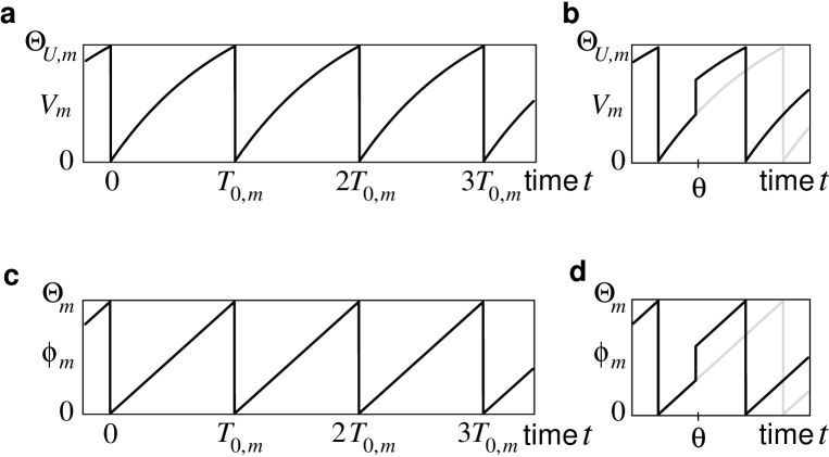
Figure 2: Relation between phase and membrane potential dynamics. (a,b) Dynamics of membrane potential $V_{m}(t)$ of neuron $m$. (a) The free dynamics is periodic with period $T_{0,m}$; (b) dynamics in response to an incoming excitatory spike at time $\theta$. (c,d) Dynamics of $\phi_{m}(t)$ representing a phase-like variable of the membrane potential dynamics displayed in panels (a) and (b). (c) Periodic phase dynamics has the same period $T_{0,m}$; (d) dynamics in response to input implies phase jump given by Eq. (2).

In the presence of interactions, the size of the discontinuities in the phase resulting from spike receptions have to match the size of the corresponding discontinuities in the membrane potential, cf. Figs. 1 and 2. To compute the correct size, we first compute the membrane potential $V_{m}(\theta^{-})=U_{m}(\phi_{m}(\theta^{-}))$ of neuron $m$ just before the reception time $\theta$ of a spike from neuron $l$. The membrane potential after the interaction is given by $V_{m}(\theta)=U_{m}(\phi_{m}(\theta^{-}))+\varepsilon_{ml}$ due to (10). We return to the phase representation using the inverse rise function and compute the phase after the interaction

$$\phi_{m}(\theta)=U_{m}^{-1}(V_{m}(\theta))=U_{m}^{-1}(U_{m}(\phi_{m}(\theta^{-}))+\varepsilon_{ml})=H_{\varepsilon_{ml}}^{(m)}(\phi_{m}(\theta^{-})),$$ (15)

and arrive at relation (2) between the phase before and after interaction. Together with the fact that the reset levels, the thresholds and the free dynamics match due to $U_{m}^{-1}(0)=0$, Eqns. (13) and (11), this shows the equivalence of the membrane potential dynamics given by the hybrid system (10) and the phase dynamics defined in section 2.1.

As an important example, the leaky integrate-and-fire neuron, defined by $f_{m}(V)=I-\gamma V$, results in the specific form

$$U_{\textrm{IF}}(\phi)=(I/\gamma)(1-e^{-\gamma\phi}).$$ (16)

Here $I>0$ is a constant external input and $\gamma\in\mathbb{{R}}$ specifies the dissipation in the system. For normal dissipation, $\gamma>0$, $U_{\textrm{IF}}(\phi)$ is concave, $U_{\textrm{IF}}^{\prime\prime}(\phi)<0$, bounded above by $I/\gamma$ and it approaches this value for $\phi\rightarrow\infty$. Assuming $I/\gamma>\Theta_{U}$ we obtain an intrinsically oscillatory neuron. For $\gamma<0,$ $U_{\textrm{IF}}(\phi)$ is convex, $U_{\textrm{IF}}^{\prime\prime}(\phi)>0$ , and bounded below by $I/\gamma<0$. It grows exponentially with $\phi$ such that, apart from $\Theta_{U}>0$, no condition is necessary to obtain a self-oscillatory neuron. For $\gamma=0$, the dynamics of an isolated neuron is trivial and specified by $U_{\textrm{IF}}(\phi)=I\phi$. The phase-threshold (13) for a particular integrate-and-fire neuron $m$ is given by

$$\Theta_{m}=U_{m}^{-1}(\Theta_{U,m})=\gamma_{m}^{-1}\ln(I_{m}/(I_{m}-\gamma_{m}\Theta_{U,m}))$$ (17)

if the parameters are $I_{m}$ and $\gamma_{m}$; for $\gamma_{m}=0$ we have $\Theta_{m}=\Theta_{U,m}/I_{m}$, the limit $\gamma_{m}\rightarrow 0$ in (17).

Another interesting and analytically useful example is given by the biological oscillator model first introduced by Mirollo and Strogatz [25],

$$U_{\textrm{MS}}(\phi)=b^{-1}\ln(1+a^{-1}\phi),$$ (18)

$ab>0$, which result from a differential equation (10) with
$f_{m}(V)=\exp(-bV)/(ab)$. Here $U_{\textrm{MS}}(\phi)$ is concave for $a,b>0$ and convex for $a,b<0$. In the former case the domain of $U_{\text{MS}}$ is $\phi\in(-a,\infty)$, with $U_{\textrm{MS}}(\phi)\rightarrow\infty$ as $\phi\rightarrow\infty$; in the latter case the domain is $\phi\in(-\infty,|a|)$, where $U_{\text{MS}}(\phi)\rightarrow\infty$ as $\phi\nearrow|a|$. Therefore, in both cases, there are no additional conditions on $\Theta_{U}$. The threshold for the phase of a particular neuron $m$ is given by

$$\Theta_{m}=U_{m}^{-1}(\Theta_{U,m})=a_{m}(\exp(b_{m}\Theta_{U,m})-1)$$ (19)

for parameters $a_{m},b_{m}$.

We note a direct relation between neural oscillators of leaky integrate-and-fire and Mirollo-Strogatz type: the rise function of a Mirollo-Strogatz oscillator is the inverse of the rise function of a leaky integrate-and-fire neuron. For $x$ in the domain of $U_{\textrm{MS}}$ (or $U_{\textrm{IF}}^{-1}$) we have

$$U_{\textrm{MS}}(x)=\frac{1}{b}\ln(1+\frac{x}{a})=-\frac{1}{\gamma}\ln(1-\frac{\gamma}{I}x)=U_{\textrm{IF}}^{-1}(x)$$ (20)

when setting $b=-\gamma$, $a=-I/\gamma$. This can be directly verified by explicitely inverting $U_{\textrm{IF}}$. To our knowledge, this has not been noticed before but might be useful to establish equivalences for dynamical properties of networks of such neurons because the response function $H$ contains both, the rise function $U$ and its inverse $U^{-1}$, cf. Eq. (3).

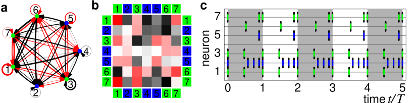
Figure 3: (color) Spike pattern in a small network ($N=7$). (a,b) Network of four leaky integrate-and-fire (green) and three Mirollo-Strogatz (blue) neurons in graph and matrix representation. The parameters of the leaky integrate-and-fire neurons are randomly chosen within $\gamma_{m}\in(0.5,1.5)$, $I_{m}=(1.08,2.08)$ and $\Theta_{m}\in(0.5,1.5)$. (If $\gamma_{m}=1$ and $I_{m}=e/(e-1)\approx 1.58$ as well as $\Theta_{m}=1$ then $\Theta_{U,m}=1$.) The parameters $b_{m}$ of the Mirollo-Strogatz neurons are randomly chosen within $b_{m}\in(0.7,1.5)$, then $a_{m}$ is chosen within $a_{m}\in(1/(e^{b_{m}}-1)-0.1,1/(e^{b_{m}}-1)+0.1)$ and $\Theta_{m}\in(0.5,1.5)$. The delays are randomly distributed within $\tau_{ml}\in(0.1,0.9)$. Connections are either excitatory (black) or inhibitory (red) . In (a) the line widths of the links, in (b) the color intensities are proportional to the coupling strengths. The network is a realization randomly drawn from those networks with couplings in the range $\varepsilon_{lm}\in(-1.5,1.5)$ that exhibit the predefined pattern displayed in (c) (black bars underlying the colored ones). (c) The spiking dynamics (green and blue bars according to neuron type) of the network shown in (a) and (b) perfectly agrees with the predefined pattern of period $T=1.3$ (black bars). The pattern includes several simultaneous spikes. One neuron, $l=4$, is silenced (non-spiking).

3 Network Design:
Analytically restricting the set of admissible networks

In this section, we explain the underlying ideas of how to design a network. For the class of systems introduced above, we derive conditions on a network under which it exhibits an arbitrary predefined periodic spike pattern. To avoid extensively many case distinctions, the following presentation requires that between any two subsequent spike times $t$ and $t^{\prime}$ of a neuron $l$ that neuron receives at least one spike in the interval $(t,t^{\prime})\cap(t,t+\Theta_{l})$. This simply ensures that all spike times in a pattern can be modified by the coupling strengths.

Definition 1

(Admissible Network) Given a predefined spike pattern, we call a network that exhibits this pattern as an invariant dynamics an admissible network.

We assume here that all neuron parameters ($U_{m}$, $\Theta_{m}$) and delay times $\tau_{ml}$ are given and fixed in a network; the task is to find networks with these given features that exhibit a desired spike pattern as an invariant dynamics. To design these networks, we choose to vary the coupling strengths $\varepsilon_{ml}$. It turns out that there is often a family of solutions such that networks with very different configurations of the coupling strengths are admissible; below we derive analytical restrictions that define the set of all networks exhibiting such a pattern. Of course there might be situations, where other parameters, such as the delays [13] are desired to be variable as well (or only). The key aspects of the approach presented below can be readily adapted to such design tasks.

The analysis presented here is very general. It covers arbitrarily large networks, different types of neurons, heterogeneously distributed delays and thresholds (and thus intrinsic neuron frequencies), combinations of inhibitory and sub- and supra-threshold excitatory interactions as well as complicated pattern dynamics that include degenerate event times, multiple spiking of the same neuron within the pattern and silent neurons that never emit a spike. Figure 3 illustrates such a general case.

3.1 Pattern Periodicity imposes restrictions

Here we provide an indexing method for any given periodic spike pattern. We then explain the relations between the periodicity of a spike pattern and the possible) periodicity of a trajectory in state space along which an appropriate network dynamical system generates that pattern.

What characterizes a periodic pattern of precisely timed spikes? Let $t_{i^{\prime}}$, $i^{\prime}\in\mathbb{Z}$, be an ordered list of times at which a neuron emits the $i^{\prime}\textrm{th}$ spike occurring in the network, such that $t_{j^{\prime}}\geq t_{i^{\prime}}$ if $j^{\prime}>i^{\prime}$. Assume a periodic pattern consists of $M$ spikes. Such a pattern is then characterized by its period $T$, by the times $t_{i}\in[0,T)$ of spikes $i\in\{1,...,M\}$ within the first period, and by the indices $s_{i}\in\{1,\ldots,N\}$ identifying the neuron that sends spike $i$ at $t_{i}\,$. If two or more neurons in the network simultaneously emit a spike, i.e. $t_{i}=t_{j}$ with $i\neq j$, the above order is not unique and we fix the corresponding indices $s_{i}$ and $s_{j}$ arbitrarily. The periodicity then entails

$$t_{i}+nT=t_{i+nM}\,\,\textrm{and}\,\,s_{i}=s_{i+nM},$$ (21)

where $n\in\mathbb{Z}$ and the definition of $s$ was appropriately extended. This imposes conditions on the time evolution of the neurons’ phases. Suppose a specific neuron $l$ fires at $K(l)$ different times $t_{i_{k}}\in[0,T)$, $k\in\{1,...,K(l)\}$ within the first period. For non-degenerate event times this implies

$$\phi_{l}(t_{i_{k}}^{-})=\Theta_{l},$$ (22)

for the neuron’s spike times, whereas at any other time $t\in[0,T)$, $t\neq t_{i_{k}}$ for all $k$,

$$\phi_{l}(t^{-})<\Theta_{l},$$ (23)

to prevent untimely firing.

Due to the periodicity of the pattern, we can assume without loss of generality that the delay times $\tau_{ml}$ are smaller than the patterns period $T$; otherwise, we take them modulo $T$ without changing the invariant dynamics such that $\tau_{ml}\in[0,T)$.

Theorem 2

The periodicity of the phases of all neurons in the network is sufficient for the periodicity of the spiking times of each neuron. If there are no supra-threshold excitations in the network, the spike pattern has the period of the phase dynamics.

If the phase dynamics is periodic with period $T$ and no supra-threshold excitations occur, it satisfies in particular $\phi_{l}((t_{i_{k}}+nT)^{-})=\Theta_{l}$ and $\phi_{l}((t+nT)^{-})<\Theta_{l}$ for $t_{i}\neq t_{i_{k}}$; $t_{i_{k}}\in[0,T)$, $k\in\{1,\ldots,K(l)\}$, are the firing times of neuron $l$ in the first period. Therefore the sub-pattern of spikes generated by neuron $l$ is periodic with period $T$. Since $l$ is arbitrary, the entire pattern is periodic with period $T$.

Interestingly, if there are supra-threshold excitations, the sub-pattern of a neuron need not have the period $T$ of the phases, as can be seen from a simple, albeit constructed example: Consider a neuron $l$, which is coupled only to itself and receives input from itself as well as once per phase period $T$ from only one other neuron $m$. If neuron $l$ receives a supra-threshold input from neuron $m$ at time $\theta$, we have $\phi_{l}(\theta^{-})<\Theta_{l}$ and $U_{l}(\phi_{l}(\theta^{-}))+\varepsilon_{lm}\geq U_{l}(\Theta_{l})$. Suppose the delay of the coupling from $l$ to $l$ is $\tau_{ll}=T$, i.e. equal to the period of the phases, and the coupling strength $\varepsilon_{ll}$ is inhibitory and such that $H_{\varepsilon_{lm}+\varepsilon_{ll}}^{(l)}(\phi_{l}(\theta^{-}))=0$, i.e. $\varepsilon_{ll}=-U_{l}(\phi_{l}(\theta^{-}))-\varepsilon_{lm}<0$. Then the phase of neuron $l$ can be periodic, whether or not it receives a spike from itself because $\phi_{l}(\theta)=0$ in each case, either due to the reset of neuron $l$ or due to the inhibitory spike received from itself. Now, if neuron $l$ sent a spike at time $\theta$, there will be no spike sending at $\theta+T$ because of the inhibition by its self-interaction. Since the self-interaction spike is then missing at time $\theta+2T$, a spike will be emitted at that later time and so on. So the spike sub-pattern of this neuron (consisting of all those spikes in the total pattern that are generated by neuron $l$) has period $2T$, and not $T$.

However the spike sub-pattern of any neuron $l$ has to be periodic even if it receives supra-threshold input. This can be seen as follows: Due to the conventions above, a spike can only be emitted when there is a discontinuity in the phase $\phi_{l}$ (after a supra-threshold excitation, the phase is always zero, after a simultaneous reception and spiking it is always unequal to $\Theta_{l}$) or if the neuron receives a supra-threshold input when its phase is $\phi_{l}(\theta^{-})=0$. Since $\phi_{l}(t)$ is piecewise continuous, in every (finite) time interval $[t,t+T)$ there are only finitely many discontinuities, as well as only finitely many times with $\phi_{l}(\theta^{-})=0$ because the phase is monotonous otherwise. Therefore, given a certain phase dynamics, spikes can be emitted by the network only at finitely many times in any interval $[t,t+T)$. This implies that there are only finitely many combinations of spikes which can be emitted by the network within a period $T$ of the phases. Thus, after a finite integer multiple of $T$, the spike patterns have to recur. After this has happened, not only the phases but (because here we can choose $T$ to be an arbitrary integer multiple of the phase period such that $\tau_{lm}<T$ without loss of generality) also all spikes in transit are the same as at some time before. Since at any time the state of the network is fixed by the phases and the spikes in transit, the entire dynamics must repeat. So, the pattern is periodic with some period $nT$, $n\in\mathbb{{N}}$.

Theorem 3

Let $S\subset\{1,...,N\}$ be the set of neurons that (i) do not receive any supra-threshold excitations and (ii) are firing at least once in the pattern. Then, the periodicity $T$ of the entire pattern is sufficient for the periodicity of the phases

$$\phi_{l}(t)=\phi_{l}(t+nT),$$ (24)

for all neurons $l\in S$, all $n\in\mathbb{Z}$ and all $t\in[0,T)$.

We disprove the opposite: Suppose, for some $l\in S$ and some $t$, $\phi_{l}(t)>\phi_{l}(t+T)$. Then this inequality remains true for all future times $t$. First, it remains true during free time evolution. Because the inputs are identical for every period and because the $H_{\varepsilon}^{(l)}(\phi)$ are strictly monotonically increasing as function of $\phi$, it remains true also after arbitrarily many interactions. Therefore, denoting the next firing time of neuron $l$ after time $t$ by $t_{j}$, we conclude that $1=\phi_{l}(t_{j}^{-})>\phi_{l}((t_{j}+T)^{-})$, violating the pattern’s periodicity. An analogous argument shows that if $\phi_{l}(t)<\phi_{l}(t+T)$ for some $t$, the pattern would not be periodic either. Therefore, if the pattern is periodic, the phases of neurons $l\in S$ are also periodic and the phases have the period of the pattern.

As direct consequence from Theorems 2 and 3 we note the important special case $S=\{1,...,N\}$.

Corollary 4

If all neurons in the network receive only subthreshold input and are firing at least once in a pattern, periodicity of the entire pattern is equivalent to the periodicity of the phase dynamics and the periods are equal.

Remark 5

If a neuron that (i) receives one or more supra-threshold inputs or (ii) is silenced (i.e. has no firing time in the pattern) has non-periodic phase dynamics, its spike sub-pattern can still be periodic.

(i) If a neuron $l$ receives a supra-threshold input, a small initial deviation from the periodic phase dynamics that occurs sufficiently briefly before the input, will only change the phase $\phi_{l}$ of that neuron but not its next spike time as long as the input remains supra-threshold. Since the dynamics continues without deviations with respect to the periodic phase dynamics, all future events will also take place at the predefined times. Thus there are initial conditions such that the phase dynamics is not entirely periodic but the spike pattern is. (ii) A sufficiently small initial deviation from the periodic phase dynamics that occurs at a silenced neuron can decay without making the neuron fire such that the spike pattern stays periodic as without the deviation, although the phase of the silenced neuron is not periodic.

For simplicity, we impose in the following that the phase dynamics of all neurons, including those neurons that are silent (i.e. never send a spike) and those that receive supra-threshold inputs, are periodic with period $T$. We consider $\phi_{l}(t)$ for $t\in[0,T)$ with periodic boundary conditions. All times are measured modulo $T$ and spike time labels $j$ are reduced to $\{1,...,M\}$ by subtracting a suitable integer multiple of $M$.

3.2 Parameterizing all admissible network designs

In this subsection we are working towards an analytical restriction of the set of all admissible networks for a given spike pattern. We provide a method of indexing all spike reception times, and of ordering them in time.The input coupling strengths are indexed accordingly. Based on this scheme, we derive conditions ensuring the sending of a spike at the pre-defined spike times, periodicity of the phase dynamics, and quiescence (non-spiking) of the neurons between their desired spike times. A main result of the paper, Theorem 7, provides a system of restrictions on the coupling strengths, which separate into disjoint constraints for the couplings onto each neuron, cf. Remark 6.

Let $\theta_{l,j}:=t_{j}+\tau_{ls_{j}}$ be the time when neuron $l$ receives the spike labeled $j$ from neuron $s_{j}$. Then, for inhomogeneous delay distribution the $\theta_{l,j}$ might not be ordered in $j$. Therefore, we define a permutation $\sigma_{l}:\{1,...,M\}\rightarrow\{1,...,M\}$ of the indices of spikes received by neuron $l$, such that

$$\bar{\theta}_{l,j}:=\theta_{l,\sigma_{l}(j)}$$ (25)

is ordered, i.e. $\bar{\theta}_{l,j}\geq\bar{\theta}_{l,i}$ if $j>i$. If multiple spikes are received at one time, $\sigma_{l}$ is not unique. This, however, has no consequence for the collective dynamics because all the associated spike receptions are treated as one according to (9).

If neuron $l$ receives multiple, say $p(l,j)$ spikes at time $\bar{\theta}_{l,j}$, we only consider the lowest of all indices $j^{\prime}$ with reception time $\bar{\theta}_{l,j^{\prime}}=\bar{\theta}_{l,j}$. If neuron $l$ receives spikes at $M_{l}$ different times, we denote the smallest index of each reception time by $j_{1}(l),...,j_{M_{l}}(l)$ such that

$$j_{n}(l):=j_{n-1}(l)+p(l,j_{n-1}(l)).$$ (26)

for $n\in\{2,\ldots,M_{l}\}$. Here $j_{1}(l)=1.$ The first set of equal reception times starts with index $j_{1}(l)=1$ and contains $p(l,1)$ spikes. Therefore, the second set of equal reception times has first index $j_{2}(l)=p(l,1)+1=p(l,j_{1}(l))+j_{1}(l)$ and contains $p(l,j_{2}(l))$ spikes. This way all indices are defined recursively.

To keep the notation concise, we skip the argument $l$ in the following (where it is clear) as the argument or index of some quantity which is itself a further index or a subindex, e.g., of $\bar{\theta}_{l}$ or $\varepsilon_{l}$. For instance, we abbreviate $\bar{\theta}_{l,j_{i}(l)}$ by $\bar{\theta}_{l,j_{i}}$ and $p(l,j_{k}(l))$ by $p(j_{k})$ where appropriate. Furthermore, indices denoting different spike receptions of neuron $l$ are reduced to $\{1,...,M_{l}\}$ by subtracting a suitable multiple of $M_{l}$. We define $P_{l}(i)\in\{1,...,M_{l}\}$ (cf. also Fig. 4) as the index of the last reception time for neuron $l$ before its firing time $t_{i}$,

$$P_{l}(i):=\text{argmin}\{t_{i}-\bar{\theta}_{l,j_{k}}\,|\,k\in\{1,...,M_{l}\},t_{i}-\bar{\theta}_{l,j_{k}}>0\}.$$ (27)

If there are no simultaneous spikes received by neuron $l$ and if there is no spike received at the firing time $t_{i}$ itself, $P_{l}(i)$ is given by

$$P_{l}(i)=\text{argmin}\{t_{i}-\bar{\theta}_{l,j}\,|\,j\in\{1,...,M\}\}.$$ (28)

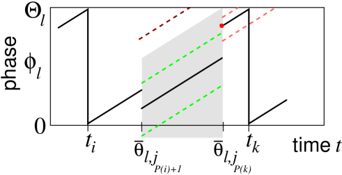
Figure 4: (color) Restriction of a neuron’s dynamics between its firing events, cf. (31) and (32). In this example, two spikes arrive between the firing times $t_{i}$ and $t_{k}$ of neuron $l$. The solid line indicates one possible time evolution of the phase $\phi_{l}(t)$. Between the firing times, $\phi_{l}(t)$ may follow any path within the possibly semi-infinite polygon (gray shaded; green dashed lines show other possible trajectories). A too large phase at $\bar{\theta}_{l,j_{P(i)+1}}$ contradicts (32) and will lead to early firing (dark red dashed line). The phase at $\bar{\theta}_{l,j_{P(k)}}$ is fixed (red dot). Any other phase inconsistent with the equality in (31) would lead to a firing time earlier or later than predefined (light red dashed lines).

In the following, if two or more reception times are equal, we will select the smallest index and restrict the dynamics only once, using Eqns. (8),(9) and the definition of $j_{i}(l)$ above. Only the total action of all spikes received by a neuron $l$ at a particular $\bar{\theta}_{l,j_{i}}$ will be restricted, by a single condition. We therefore define the sum of the coupling strengths of all spikes received by neuron $l$ at time $\bar{\theta}_{l,j_{i}}$ as

$$\bar{\varepsilon}_{l,i}=\varepsilon_{ls_{\sigma(j_{i})}}+...+\varepsilon_{ls_{\sigma(j_{i}+p(j_{i})-1)}}.$$ (29)

Indeed, $\sigma_{l}(j_{i}(l)+k)$, $k\in\{0,...,p(l,j_{i}(l))-1\}$, are the indices of the $p(l,j_{i}(l))$ different spikes received by neuron $l$ at the $i$th reception time $\bar{\theta}_{l,j_{i}}$, $i\in\{1,...,M_{l}\}$. If neuron $l$ receives all spikes at different times, we have $\bar{\varepsilon}_{l,i}=\varepsilon_{ls_{\sigma(i)}}$. Let

$$\Delta_{l,i}=\bar{\theta}_{l,j_{i+1}}-\bar{\theta}_{l,j_{i}}$$ (30)

be the time differences between two successive different reception times, where $i+1$ has to be reduced to $\{1,...,M_{l}\}$ by subtracting a suitable integer multiple of $M_{l}$. We now rewrite Eqns. (22) and (23) for neuron $l$ as a set of conditions on the phases $\phi_{l}(\bar{\theta}_{l,j_{i}})$ at the different spike reception times $\bar{\theta}_{l,j_{i}}$ in terms of the firing times $t_{i_{k}}$ of that neuron and the spike reception times $\bar{\theta}_{l,j_{i^{\prime}}}$, $i^{\prime}\in\{1,...,M_{l}\}$.

If the given pattern does not imply the reception of a spike precisely at the firing time $t_{i_{k}}$ (together with the firing times and the delays also the reception times are fixed), this results in

$$\phi_{l}(\bar{\theta}_{l,j_{P(i_{k})}})= \Theta_{l}-(t_{i_{k}}-\bar{\theta}_{l,j_{P(i_{k})}}),$$ (31)

$$\phi_{l}(\bar{\theta}_{l,j_{i}})< \Theta_{l}-\Delta{}_{l,i},$$ (32)

where $k\in\{1,...,K(l)\}$ and $i\in\{1,...,M_{l}\}\backslash\{P(i_{k})|k\in\{1,...,K(l)\}\}$. We note that, by definition (27), there is no input to neuron $l$ between the spike(s) received at $\bar{\theta}_{l,j_{P(i_{k})}}$ and the neuron’s next firing time $t_{i_{k}}$.

The firing time condition (31) states that the neuron at time $\bar{\theta}_{l,j_{P(i_{k})}}$ is as far away from its threshold $\Theta_{l}$ as it needs to be in order to exactly evolve there freely in the remaining time $t_{i_{k}}-\bar{\theta}_{l,j_{P(i_{k})}}$. The inequalities (32) guarantee that the neuron does not spike between the firing times determined by the predefined pattern: They ensure that neuron $l$ is far enough from its threshold at all other spike reception times and is not firing at any time that is not in the desired pattern, $t\neq t_{i_{k}}$.

Above, we had fixed the convention, that if a spike is received by a neuron when it is just about to fire, the spike received is processed after the sending of the new spike. If we had used the convention that first the received spike is considered, the “$<$” in inequality (32) would have been replaced by a “$\leq$”. Here equality, $\phi_{l}(\bar{\theta}_{l,j_{i}})=\Theta_{l}-\Delta{}_{l,i}$, means that the neuron approaches the threshold at $\bar{\theta}_{l,j_{i+1}}^{-}$, i.e. $\phi_{l}(\bar{\theta}_{l,j_{i+1}}^{-})=\Theta_{l},$ but since the received spike is processed first, an untimely spike can be prevented by an inhibitory input.

If there is one or several spikes received precisely at a predefined firing time $t_{i_{k}}$, supra-threshold excitation can be used to realize the pattern. To account for this, the firing time condition (31) and the silence condition (32) with $i=P_{l}(i_{k})+1$ have to be replaced by the conditions

$$\phi_{l}(\bar{\theta}_{l,j_{P(i_{k})}}) <\Theta_{l}-(t_{i_{k}}-\bar{\theta}_{l,j_{P(i_{k})}}),$$ (33)

$$U_{l}(\phi_{l}(t_{i_{k}}^{-}))+\bar{\varepsilon}_{l,P(i_{k})+1} \geq U_{l}(\Theta_{l}).$$ (34)

Here, the strict inequality (33) prevents untimely spiking (cf. the dark red dashed line in Fig. 4) and guarantees that the neuron does not reach the threshold by its intrinsic dynamics. The second, inequality (34), ensures the spiking at $t_{i_{k}}$. However, (34) is not an inequality on the phases depending at the reception times only, but involves the total coupling of the incoming spikes. We note that expression (33) with an equal sign, “$=$”, describes the case that the neuron spikes without supra-threshold excitation, because due to our above convention, the firing is treated before the spike reception. Then, inequality (34) is obsolete. So Eq. (31) is the appropriate spike time condition also if spikes are received by neuron $l$ when it just reaches threshold. Now, there are two cases possible (i) the spikes do not cause a supra-threshold excitation $U_{l}(0)+\bar{\varepsilon}_{l,P(i_{k})+1}<U_{l}(\Theta_{l})$ from the reset phase of the neuron or (ii) they cause a supra-threshold excitation, $U_{l}(0)+\bar{\varepsilon}_{l,P(i_{k})+1}\geq U_{l}(\Theta_{l})$. In the first case, $\phi_{l}(t_{i_{k}})=\phi_{l}(\bar{\theta}_{l,j_{P(i_{k})+1}})=H^{(l)}_{\bar{\varepsilon}_{l,P(i_{k})+1}}(0),$ in the second $\phi_{l}(t_{i_{k}})=\phi_{l}(\bar{\theta}_{l,j_{P(i_{k})+1}})=0$. In the first case, the silence condition (32) with $i=P(i_{k})+1$ applies such that this case does not need a special treatment, in the second, we have the inequality $\bar{\varepsilon}_{l,P(i_{k})+1}\geq U_{l}(\Theta_{l})$ instead.

Specifying conditions on the phases at these ordered and clustered (simultaneous) spike reception times is equivalent to specifying the phases at the unordered and unclustered times because $\phi_{l}(\theta_{l,i})=\phi_{l}(\theta_{l,j})$ if $\theta_{l,i}=\theta_{l,j}$.

If there are no simultaneous events, the strengths of coupling onto a particular neuron $l$, $\varepsilon_{ll^{\prime}}$, $l^{\prime}\in\{1,\ldots,N\}$, are restricted by $K(l)$ nonlinear equations and $M-K(l)$ inequalities originating from (31) and (32). All the coupling strengths in the network realizing a given pattern are thus restricted by a system of $\sum_{l=1}^{N}K(l)=M$ nonlinear equations and $\sum_{l=1}^{N}(M-K(l))=(N-1)M$ inequalities.

Remark 6

The constraints (equations and inequalities) restricting the coupling strengths of the network (to be consistent with a predefined pattern) separate into disjoint constraints for the couplings onto each individual neuron.

In the presence of simultaneous events, for each neuron there are $M_{l}-K(l)+S(l)$ inequalities originating from (33), (34) and (32), (where $S(l)$ is the number of supra-threshold excitations, not counting the ones where the spike is omitted) and $K(l)-S(l)$ equations originating from the spikings described by (31). We see that simultaneous receptions decrease the number of constraints. Again, these constraints separate (remark 6). This property is due to the fact that the pattern is fixed; it turns out (see below) that because of this separation, it is easier to find a solution for the coupling strengths that satisfy these constraints.

Fig. 4 illustrates the constraints. After a firing of neuron $l$ at time $t_{i}$ where its phase is zero, conditions (31) and (32) impose restrictions on the phases at the spike reception times while the time evolution proceeds towards the subsequent firing time $t_{k}$ of neuron $l$.

If we now compute explicitely the dynamics of neuron $l$ between two successive firing times $t_{i}$ and $t_{k}$ and evaluate the dynamics at the times occurring in (31) and (32), we obtain

$$\begin{array}[]{rl}H_{\bar{\varepsilon}_{l,P(i)+1}}^{(l)}(\bar{\theta}_{l,j_{P(i)+1}}-t_{i})&<\Theta_{l}-\Delta{}_{l,P(i)+1}\,,\\ H_{\bar{\varepsilon}_{l,P(i)+2}}^{(l)}(H_{\bar{\varepsilon}_{l,P(i)+1}}^{(l)}(\bar{\theta}_{l,j_{P(i)+1}}-t_{i})+\Delta{}_{l,P(i)+1})&<\Theta_{l}-\Delta{}_{l,P(i)+2}\,,\\ &\,\,\vdots\\ H_{\bar{\varepsilon}_{l,P(k)}}^{(l)}(...H_{\bar{\varepsilon}_{l,P(i)+2}}^{(l)}(H_{\bar{\varepsilon}_{l,P(i)+1}}^{(l)}(\bar{\theta}_{l,j_{P(i)+1}}-t_{i})+\Delta{}_{l,P(i)+1})\\ \ldots+\Delta{}_{l,\textrm{}P(k)-1})&=\Theta_{l}-(t_{k}-\bar{\theta}_{l,j_{P(k)}})\end{array}$$ (35)

in the case of no spike reception at time $t_{i}$ and no supra-threshold excitation that generates the spike at $t_{k}$.

Now we consider the case that there was a spike reception at time $t_{i}$. If a supra-threshold spike generated the spike time $t_{i}$ from a phase $\phi_{l}(t_{i}^{-})<\Theta_{l}$ and the intrinsic dynamics generates the spike at $t_{k}$, the set of equations and inequalities reads

$$\begin{array}[]{rl}H_{\bar{\varepsilon}_{l,P(i)+2}}^{(l)}(\Delta{}_{l,P(i)+1})&<\Theta_{l}-\Delta{}_{l,P(i)+2}\,,\\ &\,\,\vdots\\ H_{\bar{\varepsilon}_{l,P(k)}}^{(l)}(...H_{\bar{\varepsilon}_{l,P(i)+2}}^{(l)}(\Delta{}_{l,P(i)+1})\ldots+\Delta{}_{l,P(k)-1})&=\Theta_{l}-(t_{k}-\bar{\theta}_{l,j_{P(k)}}).\end{array}$$ (36)

Alternatively, at $t_{i}$, the threshold can be reached by the intrinsic dynamics $\phi_{l}(t_{i}^{-})=\Theta_{l}$ although a spike is arriving. Here we have to consider two different cases: (i) $U_{l}(0)+\bar{\varepsilon}_{l,P(i)+1}<U_{l}(\Theta_{l})$, i.e. the spike is subthreshold. This is just a special case of (35) with $\bar{\theta}_{l,j_{P(i)+1}}-t_{i}=0$. (ii) $U_{l}(0)+\bar{\varepsilon}_{l,P(i)+1}\geq U_{l}(\Theta_{l})$, i.e. the spike is supra-threshold. In this case, we fixed the convention that the second spike is omitted and the neuron is reset to zero; therefore system (36) is supplemented with the condition

$$\bar{\varepsilon}_{l,P(i)+1}\geq U_{l}(\Theta_{l})$$ (37)

on $\bar{\varepsilon}_{l,P(i)+1}$.

The above equations also cover the case that a spike is received by neuron $l$ at the spike time $t_{k}$ when neuron $l$ already reached $\Theta_{l}$, i.e. $\bar{\theta}_{l,j_{P(k)+1}}=t_{k}$. However, also supra-threshold excitation can then also be used to generate the spike $t_{k}$. Then, if no spike is received at $t_{i}$, or if a spike is received when the threshold is already reached and no supra-threshold excitation takes place, the couplings are restricted by (35) where the last equation has to be replaced by the inequalities

$$H_{\bar{\varepsilon}_{l,P(k)}}^{(l)}(...H_{\bar{\varepsilon}_{l,P(i)+2}}^{(l)}(H_{\bar{\varepsilon}_{l,P(i)+1}}^{(l)}(\bar{\theta}_{l,j_{P(i)+1}}-t_{i})$$

$$+\Delta{}_{l,P(i)+1})\ldots+\Delta{}_{l,P(k)-1}) <\Theta_{l}-(t_{k}-\bar{\theta}_{l,j_{P(k)}}),$$

$$U_{l}(H_{\bar{\varepsilon}_{l,P(k)}}^{(l)}(...H_{\bar{\varepsilon}_{l,P(i)+2}}^{(l)}(H_{\bar{\varepsilon}_{l,P(i)+1}}^{(l)}(\bar{\theta}_{l,j_{P(i)+1}}-t_{i})$$

$$+\Delta{}_{l,P(i)+1})\ldots+\Delta{}_{l,P(k)-1})+\Delta{}_{l,P(k)})+\bar{\varepsilon}_{l,P(k)+1} \geq U_{l}(\Theta_{l}).$$ (38)

If supra-threshold excitation occurred at time $t_{i}$ and supra-threshold input generated the spike at $t_{k}$, the couplings are restricted by (36) (possibly completed by (37)), where the last equation has to be replaced by the inequalities

$$H_{\bar{\varepsilon}_{l,P(k)}}^{(l)}(...H_{\bar{\varepsilon}_{l,P(i)+2}}^{(l)}(\Delta{}_{l,P(i)+1})$$

$$\ldots+\Delta{}_{l,P(k)-1}) <\Theta_{l}-(t_{k}-\bar{\theta}_{l,j_{P(k)}}),$$

$$U_{l}(H_{\bar{\varepsilon}_{l,P(k)}}^{(l)}(...H_{\bar{\varepsilon}_{l,P(i)+2}}^{(l)}(\Delta{}_{l,P(i)+1})$$

$$\ldots+\Delta{}_{l,P(k)-1})+\Delta{}_{l,P(k)})+\bar{\varepsilon}_{l,P(k)+1} \geq U_{l}(\Theta_{l}).$$ (39)

We have thus shown:

Theorem 7

The set of solutions to the systems (35)–(39) for all $K(l)$ pairs of subsequent firing times $(t_{i},t_{k})$, where $i=i_{n}$, $k=i_{n+1}$, $n\in\{1,\ldots,K(l)\}$, provides the set of all admissible coupling strengths $\varepsilon_{ll^{\prime}}$, $l^{\prime}\in\{1,\ldots,N\}$, of incoming connections to neuron $l$.

Corollary 8

Solutions to systems analogous to (35)–(39) for all neurons $l\in\{1,\ldots,N\}$ define all coupling strengths of an admissible network.

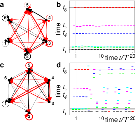
Figure 5: (color online) Two different networks (a), (c) realize the same predefined pattern ((b), (d) grey lines). The networks consist of six identical leaky integrate-and-fire neurons with $I_{m}=1.2$, $\gamma_{m}=1$, $\Theta_{m}=1$. The networks are realizations of random graphs where each coupling is present with probability $p=0.8$; the coupling delay is $\tau_{ml}=0.125$. A small random perturbation is applied at the beginning of the second period. The network dynamics (spike times relative to the spikes of neuron $l=1$, color coded for each neuron), found by exact numerical integration [35] shows that in network (a) the pattern is stable and thus regained after a few periods (b); in network (c) the pattern is unstable and eventually another pattern is assumed (d). Reproduced from Ref. [23].

Often (35)–(39) are under-determined systems such that many solutions exist, implying that many different networks realize the same predefined pattern, cf. Fig. 5. This is illustrated in more detail in the next section. Roughly speaking, in the absence of supra-threshold excitation, the time of each spike of each neuron provides one “hard” (equality) constraint on the in general N-dimensional set of input coupling strengths of that neuron. The silence conditions provide “soft” (inequality) constraints, often not lowering the dimensionality of the solution space of coupling strengths. Intuitively a hard restriction can be understood by considering a simple example: Consider a network of $N=3$ neurons. If one neuron $m$ receives two spikes in a fixed time interval in which it does not send a spike itself, the coupling strengths of these spikes are arbitrary as long as their total impact on the neuron’s phase $\phi_{m}$ (advancing or retarding) is the same, cf. also Fig. 4. This provides one, and not two, hard restrictions to the set of input coupling strengths to neuron $m$.

In the case of leaky integrate-and-fire or Mirollo-Strogatz neurons, a solution of (35)–(39), if one exists, can be found in a simple way, because the system is then reducible to be linear in the coupling strengths or polynomial in its exponentials, respectively.

Remark 9

There are patterns for which the systems (35)–(39), with predefined neuron properties and predefined delay distribution, do not have a solution.

This means that if the delays and neural parameters are specified, no network, independent of how the coupling strengths are chosen, exhibits that predefined pattern. This can already be observed from a simple example: consider a non-degenerate pattern where neuron $l$ sends three successive spikes and between each two successive of these spike times there is precisely one spike received, each sent by the same neuron $m$. Then, the coupling strength $\varepsilon_{lm}$ is fixed (by the firing time condition to which (35) reduces) to ensure the correct time of the second spike of neuron $l$ and cannot be modified to ensure the third one. So, if the interval between the second and third spike time does not by coincidence match the one determined by the input, the pattern will not be realizable by any network. Other, more complicated examples follow immediately.

This implies that certain predefined patterns may not be realizable in any network, no matter how its neurons are interconnected. We note that if we allow the neural parameters and delay times to vary as well, the system again might have a solution.

3.3 Explicit analytical parameterization

In this sub-section, we will show that an entire class of patterns can, under few weak requirements always be realized by a (typically multi-dimensional) family of networks. This class consists of simple periodic patterns, in which every neuron fires exactly once before the pattern repeats. For a simple periodic pattern, we label, without loss of generality, the neuron firing at time $t_{l}$ by $l$, i.e. $s_{l}=l$ for $l\in\{1,...,M=N\}$. Accordingly we have $\theta_{l,m}=t_{m}+\tau_{lm}$. The time differences between two successive spike times of the same neuron equal the period of the simple periodic pattern. Thus, for each neuron $l$ the reception times of spikes from all neurons of the network are guaranteed to lie between two successive firings of neuron $l$. We note again, that due to the periodicity of the pattern, we can assume without loss of generality that the delay times are smaller than the patterns period; otherwise, we take them modulo $T$ without changing the invariant dynamics. In the following, we require that two simple criteria are met.

Criterion 10

For each neuron its self-interaction delay is smaller than its free period, i.e. $\tau_{ll}<T_{0,l}$ for $l\in\{1,\ldots,N\}$.

This criterion ensures that the spike time of each neuron can be modified, at least by the self-coupling. If, as we assume throughout the manuscript (see section 3), a neuron $l$ firing only once in the period (here at $t_{l}$) receives at least one spike in the interval $(t_{l},t_{l}+\Theta_{l})$ (or, if $\Theta_{l}\geq T$ in $(t_{l},t_{l}+T)$), this criterion is not necessary to hold for Theorem 12 below; Theorem 12 holds for any presynaptic neuron sending the spike modifying the spike time (Criterion 11 appropriately modified).

Criterion 11

The threshold minus a possible lower bound of the phase plus the self-interaction delay for each neuron $l$ is larger than the pattern’s period, $\Theta_{l}-B_{l}+\tau_{ll}>T$.

This second condition is obsolete if there is no lower bound of the phase, as e.g. for leaky integrate-and-fire neurons.

Given these weak constraints, the following statement holds.

Theorem 12

For simple periodic patterns, if conditions (10) and (11) are satisfied, solutions to (35) exist and the set of admissible networks contains an $N(N-1)$ dimensional submanifold in the space of coupling strengths.

This means that all simple periodic patterns are typically realizable by a high-dimensional family of networks.

We first show that one solution exists, then state another Theorem, which explicitly shows that the solution space contains an $N(N-1)$-dimensional submanifold.

We explicitly construct a trivial solution, where only self-interaction is present, while all the other coupling strengths are zero. We consider the one neuron system consisting of neuron $l$. Because of $\phi_{l}(t_{l})=0$ and condition (10) at the reception time of the spike from neuron $l$ to itself, $\phi_{l}((t_{l}+\tau_{ll})^{-})=\tau_{ll}$ holds. At time $t_{l}+\tau_{ll}$ the neuron’s phase is set to $\phi_{l}(t_{l}+\tau_{ll})=\Theta_{l}-(T-\tau_{ll})<\Theta_{l}$ by choosing the coupling strength $\varepsilon_{ll}=H_{\phi_{l}(t_{l}+\tau_{ll})}^{(l)-1}(\phi_{l}((t_{l}+\tau_{ll})^{-}))$. Here, $H_{\psi}^{(l)-1}(\phi)=U_{l}(\psi)-U_{l}(\phi)$ is the inverse of $H_{\varepsilon}^{(l)}(\phi)$ with respect to $\varepsilon$, which exists for any $\psi$ and $\phi$ in the domain of $U_{l}$. Indeed, $0\leq\phi_{l}((t_{l}+\tau_{ll})^{-})<\Theta_{l}$ is in the domain of $U_{l}$ as well as $\phi_{l}(t_{l}+\tau_{ll})$. The latter is true, even if a lower bound is present, because $\phi_{l}(t_{l}+\tau_{ll})=\Theta_{l}-(T-\tau_{ll})>B_{l}$ due to condition 11. Now, since no further spike is received, the condition Eq. (31) for the spike sending time is satisfied and the next spiking will take place at $t_{l}+T$. Since there are no further spike receptions there are no silence conditions (32) to be satisfied. All neurons taken together as a network without couplings between different neurons the pattern is invariant. We now set out to parameterize the entire nonempty class of solutions realizing the given pattern. Indeed, for simple periodic patterns this can be done analytically:

Theorem 13

For any simple periodic pattern, the set of all networks satisfying the systems (35-39) can be explicitly parameterized.

The parameterization for each neuron $l\in\{1,\ldots,N\}$ is given as follows

(i) in the case $\theta_{l,j}\neq t_{l}$ for all $j\in\{1,...,N\}$,

$$\bar{\varepsilon}_{l,P(l)+1}= H_{\phi_{l}(\bar{\theta}_{l,j_{P(l)+1}})}^{(l)-1}(\bar{\theta}_{l,j_{P(l)+1}}-t_{l}),$$

$$\bar{\varepsilon}_{l,P(l)+k}= H_{\phi_{l}(\bar{\theta}_{l,j_{P(l)+k}})}^{(l)-1}(\phi_{l}(\bar{\theta}_{l,j_{P(l)+k-1}})+\Delta_{l,P(l)+k-1}),$$

$$\bar{\varepsilon}_{l,P(l)}= H_{\Theta_{l}-(t_{l}-\bar{\theta}_{l,j_{P(l)}})}^{(l)-1}(\phi_{l}(\bar{\theta}_{l,j_{P(l)-1}})+\Delta_{l,P(l)-1}),$$ (40)

where $k\in\{2,...,M_{l}-1\}$ and the neurons’ phases $\phi_{l}(\bar{\theta}_{l,j_{i}})$, $i\in\{1,...,M_{l}\}\backslash\{P_{l}(l)\}$ at the spike reception times are the parameters that are subject to the restrictions (32). These equations also hold with $\bar{\theta}_{l,j_{P(l)+1}}-t_{l}=0$ if there is a spike reception at $t_{l}$ but no supra-threshold excitation.

(ii) If there is a spike reception at $t_{l}$, neuron $l$ already reaches threshold due to its intrinsic dynamics $\phi_{l}(t_{l}^{-})=\Theta_{l}$, and there is supra-threshold excitation immediately after the reset, we have

$$\bar{\varepsilon}_{l,P(l)+1}\geq U_{l}(\Theta_{l})-U_{l}(0),$$

$$\bar{\varepsilon}_{l,P(l)+2}= H_{\phi_{l}(\bar{\theta}_{l,j_{P(l)+2}})}^{(l)-1}(\bar{\theta}{}_{l,j_{P(l)+2}}-t_{l}),$$

$$\bar{\varepsilon}_{l,P(l)+k}= H_{\phi_{l}(\bar{\theta}_{l,j_{P(l)+k}})}^{(l)-1}(\phi_{l}(\bar{\theta}_{l,j_{P(l)+k-1}})+\Delta_{l,P(l)+k-1}),$$

$$\bar{\varepsilon}_{l,P(l)}= H_{\Theta_{l}-(t_{l}-\bar{\theta}_{l,j_{P(l)}})}^{(l)-1}(\phi_{l}(\bar{\theta}_{l,j_{P(l)-1}})+\Delta_{l,P(l)-1}),$$ (41)

where $k\in\{3,...,M_{l}-1\}$. The parameters are the neurons’ phases $\phi_{l}(\bar{\theta}_{l,j_{i}})$, $i\in\{1,...,M_{l}\}\backslash\{P_{l}(l),P_{l}(l)+1\}$ at the spike reception times that are subject to the restrictions (32) and $\bar{\varepsilon}_{l,P(l)+1}$ which is bounded below by $\bar{\varepsilon}_{l,P(l)+1}\geq U_{l}(\Theta_{l})$.

(iii) If there is a spike reception at $\theta_{l,j}=t_{l}$, and the spike at $t_{l}$ is generated by supra-threshold excitation:

$$\bar{\varepsilon}_{l,P(l)+2}= H_{\phi_{l}(\bar{\theta}_{l,j_{P(l)+2}})}^{(l)-1}(\bar{\theta}_{l,j_{P(l)+2}}-t_{l}),$$

$$\bar{\varepsilon}_{l,P(l)+k}= H_{\phi_{l}(\bar{\theta}_{l,j_{P(l)+k}})}^{(l)-1}(\phi_{l}(\bar{\theta}_{l,j_{P(l)+k-1}})+\Delta_{l,P(l)+k-1}),$$

$$\bar{\varepsilon}_{l,P(l)+1}\geq U_{l}(\Theta_{l})-U_{l}(\phi_{l}(\bar{\theta}_{l,j_{P(l)}})+\Delta_{l,P(l)}),$$ (42)

where $k\in\{3,...,M_{l}\}$. Here the parameters are the neurons’ phases $\phi_{l}(\bar{\theta}_{l,j_{i}})$, $i\in\{1,...,M_{l}\}\backslash\{P_{l}(l)+1\}$ at the spike reception times that are subject to the restrictions (32), (33) and $\bar{\varepsilon}_{l,P(l)+1}$, which is not parameterized but only bounded below by a function of $\phi_{l}(\bar{\theta}_{l,j_{P(l)}})$ unless we require that the spike precisely excites the neuron to the threshold, i.e. the “$=$” in the last equation is valid.

These relations follow directly from (35-39) by inversion and (31-33).

Since the $\bar{\varepsilon}_{l,i}$ are disjoint sums of couplings $\varepsilon_{lj}$ , the couplings towards neuron $l$ can be parameterized using the parameters for $\bar{\varepsilon}_{l,i}$ and $p(l,j_{i})-1$ independent couplings per reception time $\bar{\theta}_{l,j_{i}}$.

We now demonstrate the second statement of Theorem 12.

In case (i) above, the Jacobian of the couplings with respect to the phases can be directly seen to have full rank $M_{l}-1$. Therefore, parameterization (40) gives an $M_{l}-1$-dimensional submanifold of the $M_{l}$-dimensional space of $\bar{\varepsilon}_{l,i}$. Since the $\bar{\varepsilon}_{l,i}$ are just disjoint sums of couplings $\varepsilon_{lj}$, an $(N-1)$-dimensional submanifold of networks realizing the pattern exists in $N$-dimensional $\varepsilon_{lj}$-space, $j\in\{1,\ldots,N\}$, $l$ fixed. We further know that the trivial solution of uncoupled neurons with self-interaction constructed above is contained in case (i). Therefore, the set of parameters subject to the restrictions (32) is nonempty. Since it is open, there is an $(N-1)$-dimensional open set parameterizing the submanifold. The product of these submanifolds of all couplings is an $N(N-1)$-dimensional submanifold which is contained in the set of solutions.

3.4 A note on stability

Is a pattern emerging in a heterogeneous network stable or unstable? We numerically investigated patterns in a variety of networks and found that in general the stability properties of a pattern depend on the details of the network it is realized in, see Fig. 5 for an illustration. Depending on the network architecture, the same pattern can be exponentially stable or unstable, or exhibit oscillatory stable or unstable dynamics.

For any specific pattern in any specific network, the linear stability properties can also be determined analytically, similar to the exact perturbation analyses for much simpler dynamics in more homogeneous networks [33, 34]. More generally, in every network of neurons with congenerically curved rise functions and with purely inhibitory (or purely excitatory) coupling, a nonlinear stability analysis [21] shows that the possible non-degenerate patterns are either all stable or all unstable. For instance, in purely inhibitory networks of neurons with rise functions of negative curvature, such as standard leaky integrate-and-fire neurons, Eq. (16) with $\gamma>0$, every periodic non-degenerate spike pattern, no matter how complicated, is stable.

If in the pattern, a neuron receives a spike when it was just about to spike and the corresponding input coupling strength is not zero, the pattern is super-unstable: an arbitrarily small perturbation in the reception time can lead to a large change in the dynamics. These cases, however, are very atypically in the sense that when randomly drawing the delay times and the spike times in a pattern from a smooth distribution the probability of occurrence of any simultaneous events, in particular those leading to this super-instability, is zero. Simultaneous spikes sent and simultaneous spike received by different neurons do not lead to a super-unstable pattern, because the phase dynamics depends continuously on perturbations.

4 Implementing additional requirements:
Network Design on Predefined Connectivities

4.1 Can we require further system properties?

As we have seen above, the systems of equations and inequalities (35)–(39) defining the set of admissible networks is often underdetermined. We can then require additional properties from the neurons and their interactions. So far we assumed that neurons and delays were given but arbitrary, but network coupling strengths, and therefore the connectivity, were not restricted.

Here we provide examples of how to require in advance additional features that are controlled by the coupling strengths. A connection from a neuron $l$ to $m$ can be absent (requiring the coupling strength $\varepsilon_{ml}=0$), taken to be inhibitory ($\varepsilon_{ml}<0$) or excitatory ($\varepsilon_{ml}>0$) or to lie within an interval; in particular, we can specify inhibitory and excitatory subpopulations.

Additional features entail additional conditions on the phases at the spike reception times which can be exploited for network parameterization, as we here demonstrate for simple periodic patterns, where we employ the same conventions as in sub-section 3.3.

(i) If the pattern is non-degenerate, exclusion of self-interaction is guaranteed by the conditions

$$\phi_{l}(\theta_{l,l})=\tau_{ll}$$ (43)

if there is no spike-reception in $(t_{l},\theta_{l})$, and

$$\phi_{l}(\theta_{l,l})-\phi_{l}(\theta_{l,\sigma(\sigma^{-1}(l)-1)})=\Delta_{l,\sigma^{-1}(l)-1}$$ (44)

otherwise, typically reducing the dimension of the submanifold of possible networks by $N$.

(ii) Requiring purely inhibitory networks leads to the accessibility conditions

$$\phi_{l}(\bar{\theta}_{l,j_{P(l)+1}})\leq \bar{\theta}_{l,j_{P(l)+1}}-t_{l},$$ (45)

$$\phi_{l}(\bar{\theta}_{l,j_{i+1}})-\phi_{l}(\bar{\theta}_{l,j_{i}})\leq \Delta_{l,i},$$ (46)

where $i\in\{1,...,M_{l}\}\backslash\{P_{l}(l)\}$. Since $\phi_{l}(\bar{\theta}_{l,j_{P(l)+1}}^{-})=\bar{\theta}_{l,j_{P(l)+1}}-t_{l}$, the first inequality is equivalent to $\phi_{l}(\bar{\theta}_{l,j_{P(l)+1}})\leq\phi_{l}(\bar{\theta}_{l,j_{P(l)+1}}^{-})$. This guarantees $\bar{\varepsilon}_{l,P(l)+1}=H_{\phi_{l}(\bar{\theta}_{l,j_{P(l)+1}})}^{(l)-1}\left(\phi_{l}(\bar{\theta}_{l,j_{P(l)+1}}^{-})\right)=U_{l}(\phi_{l}(\bar{\theta}_{l,j_{P(l)+1}}))-U_{l}(\phi_{l}(\bar{\theta}_{l,j_{P(l)+1}}^{-}))\leq 0,$ due to the monotonicity of $U_{l}$, such that the couplings summing up to $\bar{\varepsilon}_{l,P(l)+1}$ can be chosen to be inhibitory or zero. Analogously, the second inequality ensures $\phi_{l}(\bar{\theta}_{l,j_{i}})\leq\phi_{l}(\bar{\theta}_{l,j_{i}}^{-}).$ We note that (45) also covers the case of spikes received at time $t_{l}$. Since their action is inhibitory, no supra-threshold excitation can occur and (45) yields $\phi_{l}(t_{l})=\phi_{l}(\bar{\theta}_{l,j_{P(l)+1}})\leq\bar{\theta}_{l,j_{P(l)+1}}-t_{l}=0$.

To parameterize all networks we can therefore successively choose $\phi_{l}(\bar{\theta}_{l,j_{P(l)+m}})$, $m\in\{1,...,M_{l}-1\}$, starting with $m=1$. Inequalities (45) and (46) hold with reversed relations for purely excitatory coupling if no supra-threshold excitation occurs. Otherwise, they have to be replaced by

$$\phi_{l}(\bar{\theta}_{l,j_{P(l)+2}})\geq \bar{\theta}_{l,j_{P(l)+2}}-t_{l},$$ (47)

$$\phi_{l}(\bar{\theta}_{l,j_{i+1}})-\phi_{l}(\bar{\theta}_{l,j_{i}})\geq \Delta_{l,i},$$ (48)

where $i\in\{1,...,M_{l}\}\backslash\{P_{l}(l),P_{l}(l)+1\}$. An additional condition at time $t_{l}=\bar{\theta}_{l,j_{P(l)+1}}$ is not necessary, since the condition that the spike has a supra-threshold action already ensures the excitatory coupling. In general, purely inhibitory realizations can exist if the minimal inter-spike-interval of each single neuron $l$ is larger than the neuron’s free period, i.e.

$$\min\left\{t_{i_{k+1}}-t_{i_{k}}|k\in\{1,...,K(l)\}\right\}\geq\Theta_{l},$$ (49)

for all $l\in\{1,...,N\}$, where the index $k+1$ has to be reduced to $\{1,...,K(l)\}$ subtracting a suitable multiple of $K(l)$. If (49) is not satisfied, for some $k$, $\phi_{l}(t_{i_{k+1}}^{-})=\Theta_{l}$ is not reachable from $\phi_{l}(t_{i_{k}})=0$. For the same reason, purely excitatory realizations can exist if

$$\max\left\{t_{i_{k+1}}-t_{i_{k}}|k\in\{1,...,K(l)\}\right\}\leq\Theta_{l}.$$ (50)

In the case of simple periodic patterns, for purely inhibitory coupling the inequalities (49) reduce to $T\geq\max_{m}\Theta_{m}$. If even

$$T>\max_{m}\Theta_{m}$$ (51)

holds, the trivial solution is purely inhibitory with couplings $\varepsilon_{ll}<0$. Therefore, from Theorems 12, 13 and the corresponding proof, we conclude that there is a submanifold of purely inhibitory networks in the set of solutions. Analogously, if

$$T<\min_{m}\Theta_{m},$$ (52)

there is a submanifold of purely excitatory networks in the set of solutions.

4.2 Very different connectivities, yet the same pattern

Requiring certain connections to be absent is particularly interesting. This just enters the restricting conditions (35-39) as simple additional equalities $\varepsilon_{ml}=0$ specifying that there is no connection from $l$ to $m$.

By specifying absent connections we generally also specify which connections are present (except in cases where $\varepsilon_{ml}=0$ by coincidence), i.e. the connectivity of the network. Though very simple to implement, specifying the absence of connections is thus a very powerful tool.

Remark 14

Absence of each of the $N^{2}$ connections $\varepsilon_{ml}$, $m,l\in\{1,\ldots,N\},$ can be pre-specified independently.

This means that we can typically specify in advance any arbitrary connectivity of the network. A particular predefined pattern is of course not always realizable in such a network.

We illustrate this network design with predefined connectivities by a few examples. The two small networks of Figure 5 are both networks with pre-specified absent links. Here we chose random networks of $N=6$ neurons where each connection is present with probability $p=0.8$. The figure displays two different networks that exhibit the same pattern. One network has been chosen such that the pattern is stable the other such that it is unstable. Interestingly, on the one hand the same pattern can be invariant in two different networks with similar statistics, on the other hand their stability properties depend on the details of the coupling configurations.

We also considered large networks by predefining exactly the presence or absence of each link according to very different degree distributions. We designed them, by varying the remaining (non-zero) coupling strengths, such that all network examples exhibit the same predefined simple-periodic pattern. Network design on specific connectivities is of course not restricted to the example cases presented here, because the sets of input coupling strengths can be specified independently from each other.

For illustration, we present four large networks of $N=1000$ neurons realizing the same predefined periodic pattern of spikes. For simplicity, we took for all networks the in-degree equal to the out-degree for each neuron. A random degree sequence was drawn from the given degree distribution (see below) and the degrees assigned to the neurons. The networks were then generated using a Monte-Carlo method similar to those discussed in Ref. [24].

Approximately $50$% of the neurons are of integrate-and-fire type, the remaining are of Mirollo-Strogatz-type. The parameters of the leaky integrate-and-fire neurons are randomly chosen within $I_{m}\in(1.08,2.08)$, $\gamma_{m}\in(0.5,1.5)$, the parameters $b_{m}$ of the Mirollo-Strogatz neurons are randomly chosen in $b_{m}\in(0.9,1.2)$, then $a_{m}\in(1/(e^{b_{m}}-1)-0.1,1/(e^{b_{m}}-1)+0.1)$. The thresholds of both neuron types are uniformly distributed within the interval $\Theta_{l}\in(0.8,1.2)$. The delay distribution is heterogeneous, delays are uniformly distributed in the interval $\tau_{lm}\in(0.1,0.3)$, $l,m\in\{1,...,N\}$.

Two network examples (Figs. 6,7) have random connectivity with different exponential degree distributions

$$p(k)\propto e^{-\alpha k}$$ (53)

where $k$ is the neuron degree. The other two networks (Figs. 8,9) have power-law degree distribution, according to

$$p(k)\propto k^{-\gamma}$$ (54)

For both distributions, we fixed a lower bound on the degree $k_{c}=6$ such that each neuron has $k\geq k_{c}$ input and output connections. For networks of both distributions, we realized one with purely inhibitory coupling strengths (Figs. 6,8) and one with mixed inhibitory and excitatory coupling strengths (Figs. 7,9).

All network examples are constructed to realize the same predefined spike pattern with period $T=1.5$. The numerical simulations (Figs. 6-9c, green or blue bars for spiking integrate-and-fire or Mirollo-Strogatz-type neurons) agree perfectly with the predefined pattern (Figs. 6-9c, underlying black bars).

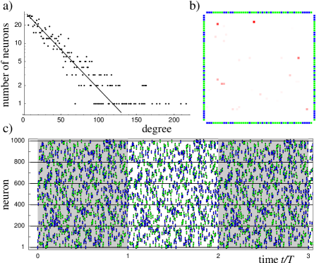
Figure 6: (color) Network design with given connectivity. Predefined pattern in a network ($N=1000$) with exponential degree distribution (panel (a), $\alpha=0.03$) and purely inhibitory coupling. Panel (b) displays the sub-matrix of coupling strengths between the first $50$ neurons. Inhibitory couplings are red, excitatory couplings are gray. The intensity of the color is proportional to the coupling strength. Due to too faint color, some very weak couplings are invisible in the plot. The frame shows integrate-and-fire neurons in green and Mirollo-Strogatz neurons in blue. (c) The numerical simulations of the designed networks (green and blue bars for integrate-and-fire and Mirollo-Strogatz type neurons) show perfect agreement with the predefined pattern (black bars).

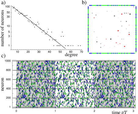
Figure 7: (color) Network design with given connectivity. Predefined pattern in a network ($N=1000$) with exponential degree distribution (panel (a), $\alpha=0.1$) and mixed inhibitory and excitatory coupling. Other panels as in Figure 6.

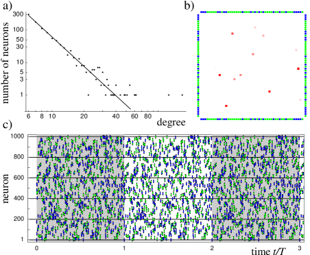
Figure 8: (color) Network design with given connectivity. Predefined pattern in a network ($N=1000$) with power-law degree distribution (panel (a), $\gamma=3.0$) and purely inhibitory coupling. Other panels as in Figure 6.

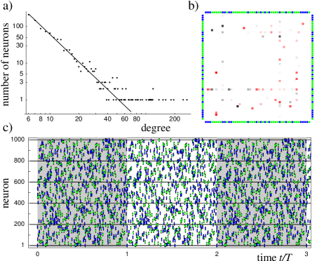
Figure 9: (color) Network design with given connectivity. Predefined pattern in a network ($N=1000$) with power-law degree distribution (panel (a), $\gamma=2.5$) and mixed inhibitory and excitatory coupling. Other panels as in Figure 6.

Remark 15

Due to the simplicity of imposing absence of links, the same method can be applied to a wide variety of network connectivities. In particular, a connectivity can be randomly drawn from any kind of degree distribution; a connectivity can also be structured (e.g. correlated degrees) and one may want to implement a very detailed specific form of it, e.g., as given by real data.

As noted above, however, not all networks can be designed for any pattern; in particular it is in general necessary to have sufficiently many incoming links to each neuron such that the interaction delay times and the input coupling strengths can account for the desired phase dynamics consistent with the predefined spike pattern.

5 Designing optimal networks

In section 3 we derived analytical constraints specifying the set of all networks that exhibit a predefined pattern and found that often there is a multi-dimensional family of solutions in the space of networks (as defined by all coupling strengths). In the previous section we exploited this freedom to design networks the connectivity of which is specified in detail. We may also exploit the freedom of choosing a solution among many possibilities by optimizing certain network properties.

Can we design networks that optimize certain structural features and at the same time exhibit a predefined pattern dynamics? This question is a very general one and it can be addressed by considering a variety of features of neuroscientific or mathematical interest. To briefly illustrate the idea, we here focus on optimizing convex ’cost’ functions of the coupling strengths $\varepsilon_{lm}$ and look for those networks among the admissible ones that minimize wiring costs.

Even for this very specific problem there are a number of different approaches we can take. For instance, we can consider networks with the same type of interactions, inhibitory or excitatory, or allow for a mixture of both, or optimize for different features of the connectivity. For simplicity, we here consider small networks whose neurons are exclusively of integrate-and-fire type and allow for a mixture of inhibitory and excitatory coupling. Integrate-and-fire neurons have the advantage (for both analysis and optimization) that the constraints (35)–(39) are linear.

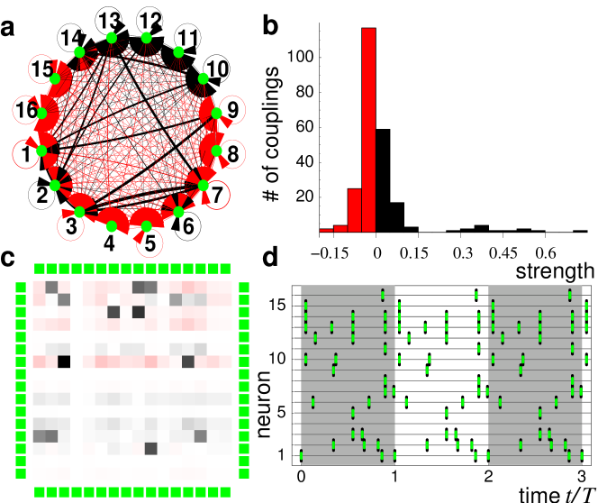
Figure 10: (color) Network of leaky integrate-and-fire neurons that minimizes the wiring cost in Euclidean norm by minimizing (55). The parameters are randomly chosen within $I_{m}\in(1.0,2.0)$, $\gamma_{m}\in(0.5,1.5)$ and $\Theta_{m}\in(0.8,1.2)$. The delays are uniformly distributed in $\tau_{lm}\in(0.1,0.9)$, $l,m\in\{1,...,N=16\}$. Panels (a) and (c) show the network and the coupling matrix $\varepsilon_{lm}$. Panel (b) shows the histogram of the strengths of existing connections in the network. The bin size is 0.05. Panel (d) displays the predefined spike pattern (black bars) that is accurately reproduced (green bars). In the optimal network every neuron is connected to every other except the silenced neuron $l=4$. This neuron has no outgoing connections: Since it generates no spikes, outgoing connections would be superfluous and do not appear in the optimal network.

The most straightforward goal for optimizing wiring costs is to minimize the quadratic cost function

$$G(\varepsilon):=\sum_{l=1}^{N}\sum_{m=1}^{N}\varepsilon_{lm}^{2}\,,$$ (55)

A similar approach has already been successfully used when minimizing wiring costs of biological neural networks based on anatomical and physical constraints but neglecting dynamics issues, see, e.g. [8]. When minimizing the Euclidian ($L_{2}$) norm $\sqrt{G(\varepsilon)}$ by minimizing (55) for each row vector $(\varepsilon_{l,m})_{m\in\{1,\ldots,N\}}$ of the coupling matrix, a solution is searched among the admissible ones that is closest to the origin in the space of networks (defined by the coupling strengths).

Figure 10 shows an example of such an optimization. The network is almost globally connected and shows moderate variation among the individual coupling strengths. The predefined pattern dynamics is exactly reproduced. Such a network, while optimizing the wiring cost according to (55) does not appear to have any special features apart from apparently homogeneous and relatively small coupling strengths.

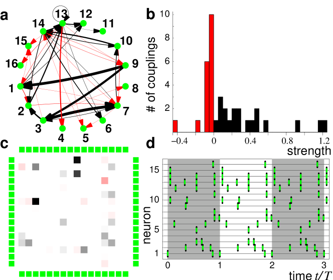
Figure 11: (color) Network that minimizes the wiring cost in $L_{1}$-norm (56). The parameters are randomly chosen within $I_{m}\in(1.0,2.0)$, $\gamma_{m}\in(0.5,1.5)$ and $\Theta_{m}\in(0.8,1.2)$. The delays are uniformly distributed in $\tau_{lm}\in(0.1,0.9)$, $l,m\in\{1,...,N=16\}$. Panels (a) and (c) show the network and the coupling matrix $\varepsilon_{lm}$. Panel (b) shows the histogram of the strengths of existing connections in the network. The bin size is 0.05. Panel (d) displays the predefined spike patterns (black bars) that is accurately reproduced (green bars). The optimal network is very sparsely connected. In fact the network has one large strongly connected component, containing the neurons $\{1,2,3,5,7,9,10,13,14\}$, while the remaining neurons receive connections exclusively from this component and do not have any outgoing connections.

It seems that nature often designs networks in a different way, possibly such that they serve a dynamical purpose especially well. In particular evolution has not optimized most biological neural networks in the above manner: they are not close to globally coupled.

An alternative goal for optimizing wiring costs is to minimize the cost function

$$G(\varepsilon):=\sum_{l=1}^{N}\sum_{m=1}^{N}\left|\varepsilon_{lm}\right|,$$ (56)

that is, the $L_{1}$-norm of each row vector of the coupling matrix. When minimizing the $L_{1}$-norm (56), as before, a solution is searched among the admissible ones that is closest to the origin in the space of networks, but this time ’close’ is defined by the $L_{1}$ distance measure. Interestingly, under weak conditions on the linear equality constraints, an optimal solution (56), searched under these constraints only, has many entries $\varepsilon_{lm}$ equal to zero, cf. [7]. Because we typically also have many inequalities which depend on details of the pattern dynamics and are therefore uncontrolled, we cannot guarantee the zero entries for the full optimization problem (defined by equalities and inequalities) here. However, our numerics suggests that the solution in fact gives a network with many links absent and the number of links present being typically of the order of number of equality constraints.

Thus a network optimized by minimizing the $L_{1}$-norm is sparse, see, e.g., Fig. 11. Moreover, compared to the optimal $L_{2}$-norm solution above, this network has more heterogeneous connection strengths. Given some type of dynamics, a sparse network possibly is what biological systems would optimize for. In biological neural networks for instance, creating an additional synapse would probably use more resources (energy, biological matter, space, time, etc.) than making an existing synapse stronger.

Sparseness might possibly also be optimized in biological neural networks where requirements are met enabling other specific, functionally relevant dynamics. In general, of course, this dynamics may or may not consist of spike patterns.

Remark 16

The optimization problem, (55) and (56) with constraints (35)–(39), does typically not have a true optimum.

If a pattern is predefined that has more than one reception times between two successive sending events of some neuron, there usually are strict inequalities among the constraints (35)–(39). Because the functions $H_{\varepsilon}^{(l)}$ in (35)–(39) are local homeomorphisms (i.e. are continuous with local inverses that are continuous) the set of admissible coupling strengths is then not closed and thus does not contain its boundary.

During optimization, typically a solution is searched that is as close to such a boundary as possible. For instance, suppose one connection from $m$ to $l$ is inhibitory and its strength $\varepsilon_{lm}$ is desired as small as possible. Then a solution is searched where the phase $\phi_{l}$ of the neuron $l$ that receives a spike from $m$ is such that the phase jump that spike induces is maximal (in absolute value) when $\varepsilon_{lm}$ is held constant. This way a given desired phase jump would be achieved by a minimal coupling strength. Typically, the phase $\phi_{l}$ sought-after corresponds to a boundary of the set of admissible phases. For instance, if $U_{l}$ is concave, an inhibitory spike has the largest possible effect on $\phi_{l}$ (largest phase jump) at $\phi_{l}=\Theta_{l}$. The corresponding phase constraint, however, may read $\phi_{l}<\Theta_{l}$. Thus the boundary phase and therefore also the boundary coupling strength cannot be assumed. As a consequence, the optimization problem has no true solution.

We fix this problem by imposing, instead of (35)–(39) and possible additional constraints with inequalities of the type $\phi_{l}>x$ or $\phi_{l}<y$, constraint sets that are closed, i.e. $\phi_{l}\geq x+\kappa$ or $\phi_{l}\leq y-\kappa$, where $\kappa>0$, $\kappa\ll 1$ is a small cutoff. We fixed $\kappa=0.001$ in the optimal design problems considered here.

6 Brief Network Design Manual

In this section we briefly summarize the presented method (of designing the coupling strengths of a network such that it realizes a pre-defined pattern) by providing step-by-step instructions. For simplicity, as above, we assume that all other parameters, such as neuron rise functions and interaction delay times are given or fixed a priori. We refer to the relevant sections and formulas derived above where appropriate. A simple example of a small network of $N=3$ neurons (Fig. 12) illustrates the indexing used in the general instructions.

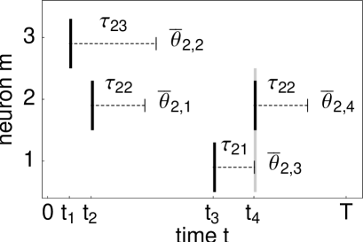
Figure 12: Pattern of $M=4$ spikes in a network of $N=3$ neurons illustrating the indexing of spike sending and reception times. The spike (sending) times $t_{i}$, marked by black bars, are indexed with increasing $i$ according to their temporal order of occurrence in the network (the neuron identities play no role for this index). The ordered spike reception times $\bar{\theta}_{l,i}$ are displayed for neuron $l=2$. They are generally different for other receiving neurons ($l\neq 2$, not shown) and obtained by adding the delay times $\tau_{lm}$ (dashed lines) to the spike sending times $t_{j}$ and then ordering the resulting set for each neuron. Here there is one degenerate event: neuron $l=2$ receives a spike from $m=1$ exactly at its second spike sending time $t_{4}$ (light gray vertical bar).

Suppose a periodic pattern of $M$ spikes is given in a network of $N$ neurons.

1) Label the neurons arbitrarily by $m\in\{1,\ldots,N\}$.

2) Fix the origin of time, $t=0$, arbitrarily and pick an interval of length $T$, the period of the given pattern.

3) Order the spike times. Some neurons may send one spike per period, others multiple spikes, and again others no spike at all (silent neuron). Label the times of all spike sending events according to their temporal order of occurrence in the network. In the example of Fig. 12, we have one spike time $t_{1}$ of neuron $m=3$, two spike times $t_{2}$ and $t_{4}$ of neuron $m=2$ and one spike time $t_{3}$ of neuron $m=1$.

4) Compute the spike reception times at each neuron $l$ using the interaction delay times $\tau_{lm}$ such that $\theta_{l,j}=t_{j}+\tau_{lm}$. Here $m$ is that neuron that sent the spike at time $t_{j}$. We identify this neuron by $s_{j}:=m$ in the formulas above. For those neurons $l$ for which the spike reception times are not ordered, reorder them by permuting indices according to (25) to obtain ordered reception times $\bar{\theta}_{l,j}$. In the example, the delay time $\tau_{23}$ from neuron $m=3$ to neuron $l=2$, is longer than $\tau_{22}$, which, for the given pattern, results in reception times $\theta_{2,j}$ that are not in the same order as the spike sending times $t_{j}$. Particularly we have $\bar{\theta}_{2,1}=\theta_{2,2}$, $\bar{\theta}_{2,2}=\theta_{2,1}$, $\bar{\theta}_{2,3}=\theta_{2,3}$ and $\bar{\theta}_{2,4}=\theta_{2,4}$. The ordered reception times $\bar{\theta}_{2,j}$ are as indicated in Figure 12.

5) Are there degenerate times at which a reception time at one neuron equals that neuron’s spike sending time? If so, decide whether to use, for each such reception, supra-threshold or sub-threshold input signals; for each non-degenerate spike reception, use sub-threshold inputs. In the example, the time at which neuron $2$ receives a spike from neuron $1$ coincides with the second spike sending time $t_{4}=\bar{\theta}_{2,3}$ of neuron $2$. So for this reception time $\bar{\theta}_{2,3}$ of neuron $l=2$, decide whether to use sub- or supra-threshold input. For all other receptions at neuron $l=2$, use sub-threshold input.

6) For each neuron $l$ and each spike time $t_{k}$ of that neuron, look for the previous spike time of neuron $l$ and name it “$t_{i}$”. Compute and look up the particular response functions $H^{(l)}_{\varepsilon}$, the thresholds $\Theta_{l}$ and the differences in spike reception times $\Delta_{l,j}$. Now, if there is

• no spike reception at time $t_{i}$ and no supra-threshold input generating $t_{k}$ write down system (35).

• a spike reception at $t_{i}$ inducing the spike at $t_{i}$ by a supra-threshold input and no supra-threshold input generating $t_{k}$, write down system (36).

• a spike reception at time $t_{i}$ but the threshold is nevertheless reached by the neuron from its intrinsic dynamics (as desired by the designer) and no supra-threshold input generating $t_{k}$ : if the coupling, effective after reset at $t_{i}$, is (i) subthreshold, this is a special case of (35); (ii) if it is supra-threshold, supplement (36) with (37).

• case (a) with supra-threshold input generating $t_{k}$ write down (35) with the equation replaced by (38).

• case (b) with supra-threshold input generating $t_{k}$ write down (36) and replace the equation by (39).

• (i) for the case (c,i) with supra-threshold input generating $t_{k}$, write down (35) and replace the equation by (38) (ii) for the case (c,ii) write down (36) completed by (37) and replace the equation by (39).

Repeat this step 6) for all neurons $l$ and all pairs $(t_{i},t_{k})$ of their successive spike times.

At this point, a complete list of restricting equations and inequalities has been created. One particular solution to these restrictions provides all coupling strengths of a network that exhibits the predefined pattern as an invariant dynamics. The set of all solutions thus provides the set of all networks that exhibit this spike pattern.

One can now either

7) solve for one particular solution; or

8) further restrict the constraint system, e.g. by requiring additional properties of the connectivity, cf. section 4, and solve that for a particular solution; or

9) use the entire constraint system and try to find a solution that is optimal in a desired sense, as done in section 5 for the example of minimal wiring costs; or

10) combine additional restrictions, point 8), and optimization, point 9).

Point 10) has not been presented in this manuscript but is an interesting starting point for future research.

We found it useful to start trying these network design methods on small network examples of simple units, for instance integrate-and-fire neurons, and investigate very simple patterns with few (or no) degeneracies first. Moreover, given that there is no general recipe about how to apply additonal restrictions and how to solve general optimization problems, it might also be useful to start with few restrictions and simple optimization tasks in very small networks the dynamics of which (and possibly their desired “optimal” features) can be understood intuitively.

7 Conclusions

7.1 Summary

In this article, we have shown how to design model networks of spiking neurons such that they exhibit a predefined dynamics. We focused on the question of how to adapt the coupling strengths in the network to fix the dynamics. We derived analytical constraints on the coupling strengths (which define the set of all networks) given an arbitrarily chosen predefined periodic spike pattern. The analysis presented here is very general. It covers networks of arbitrary size and of different types of neurons, heterogeneously distributed delays and thresholds (and thus intrinsic neuron frequencies), combinations of inhibitory and sub- and supra-threshold excitatory interactions as well as complicated stored patterns that include degenerate event times, multiple spiking of the same neuron within the pattern and silent neurons that never fire. These constraints do not admit a solution for certain patterns. Once the features of individual neurons and the delay-distribution are fixed, this implies that these patterns cannot exist in any network, no matter how the neurons are interconnected.

A predefined simple periodic pattern is particularly interesting because under weak assumptions, the constraint system has a solution for any such pattern. Thus, a network realizing any simple periodic pattern is typically guaranteed to exist; we analytically parameterized all such networks. The family of solutions is typically high-dimensional, cf. also [38], and we showed how to design networks that are further constraint. We highlighted the possibility to design networks of completely predetermined connectivity (fixing the absence or presence of links between each pair of neurons). To illustrate the idea, we have explicitely designed networks with different exponential and power-law degree distributions such that they exhibit the same spike pattern.

The design perspective can furthermore be used to find networks that exhibit a predefined dynamics and are at the same time optimized in some way. As a first example, we considered networks minimizing wiring cost. The connectivity of biological neural networks that exhibit precise spatio-temporal spiking dynamics is typically sparse. The work presented here suggests that this sparseness may result from an optimization process that takes into account dynamical aspects. If biological neural networks indeed optimize connectivity for dynamical purposes, our results suggest that these networks may minimize the total number of connections (rather than, e.g., their total strengths) and at the same time still realize specific spiking dynamics.

7.2 Perspectives for future research

The dynamics of artifically grown biological neural networks may provide an immediate application ground for the theory presented here. For instance, to uncover the origin of recurring, specific spike patterns, one could imagine using a design approach to precisely control the growth of biological neural networks on artificial substrates and reveal under which conditions and how a desired pattern arises in a biological environment. For practicability of such an approach, of course, pattern stability, only briefly discussed here, needs a more detailed analysis. Moreover, the size of the basin of attraction of a spike pattern will probably also play an important role in such studies. Perhaps it may even become possible to develop design techniques to optimize pattern stability and basin size, thus gaining robust pattern dynamics.

Network design might be a valuable new perspective of research, as shown here by example for spiking neural networks. Using the design idea might not only aid a better understanding of the relations between structure and function of complex networks in general; network design might also be exploited for systems that we would like to fulfill a certain task, for example computational systems such as artificial neural networks.

The idea of designing a system of coupled units is not new. For instance an artificial Hopfield neural network [16] can be trained by gradually adapting the coupling strengths, such that it becomes an associative memory, fulfilling a certain pattern recognition task. Such networks typically consist of binary units that are all-to-all coupled. However, already in the late 1980’s [6] mean field theory has been successfully extended to study the properties of sparse, randomly diluted Hopfield networks. In that work, Derrida, Gardner and Zippelius showed that the storage capacity of such diluted systems is reduced compared to the all-to-all coupled one, but still significant.

Here we transferred the idea of system design to complex networks that may have a complicated, irregular connectivity and thus cannot in general be described by mean field theory. In related study [39], a method has been presented to construct neural network models that exhibit spike trains with high statistical correlation to given extracellular recordings. The specific results presented our this study might be valuable to obtain further insights into biological neural systems and the precisely timed, still unexplained, spike patterns they exhibit. This study, however, also raises a number of questions both for the theory of spiking neural network as well as, more generally, for studies of other complex networks and their dynamics. We list a few questions we believe are among the most interesting, and promising in the near future:

Can network design studies help to develop functionally relevant dynamics? Design of particular model networks could on the one hand identify possible functional (as well as irrelevant) subgroups of real-world networks, including neural, gene and social interaction networks; on the other hand network design could also guide the development of new useful paradigms and devices, for instance for information processing or communication networks.

What is an optimal network design that ensures synchronization [28], a prominent kind of collective dynamics? The approach could of course also be useful to avoid certain behavior. For instance, may network design even give hints about how to suppress synchronization and hinder epileptic seizures in the brain (see e.g. [27] and references therein)? What are potential ways to design your favorite network? What kind of dynamics would be desirable (or undesirable^∗) for it.

Let’s use network design – and make specific network dynamics (not^∗) happen.

References

- [1] M. Abeles. Local Cortical Circuits: An Electrophysiological Study. Springer, Berlin, 1982.
- [2] M. Abeles. Time is precious. Science 304:523, 2004.
- [3] T. Achacoso and W. Yamamoto, editors. AY’s Neuroanatomy of C. elegans for computation. CRC Press, 1992.
- [4] P. Ashwin and M. Timme. Unstable attractors: existence and robustness in networks of oscillators with delayed pulse coupling. Nonlinearity 18:2035, 2005.
- [5] Y. Aviel, C. Mehring, M. Abeles, and D. Horn. On embedding synfire chains in a balanced network. Neural Comput. 15:1321, 2003.
- [6] A. Zippelius, B. Derrida, E. Gardner. An exactly solvable asymmetric neural network model. Europhys. Lett. 4:167, 1987.
- [7] S. Boyd and L. Vandenberghe. Convex Optimization. Cambridge Univ. Press, Cabridge, UK, 2004.
- [8] D. B. Chklovskii. Exact solution for the optimal neuronal layout problem. Neural Comput. 16:2067, 2004.
- [9] M. Denker, M. Timme, M. Diesmann, F. Wolf, and T. Geisel. Breaking synchrony by heterogeneity in complex networks. Phys. Rev. Lett. 92:074103, 2004.
- [10] M. Diesmann, M.-O. Gewaltig, and A. Aertsen. Stable propagation of synchronous spiking in cortical neural networks. Nature 402:529, 1999.
- [11] B. Drossel and A. McKane. Modelling Food Webs. Wiley-VCH, 2002.
- [12] U. Ernst, K. Pawelzik, and T. Geisel. Synchronization induced by temporal delays in pulse-coupled oscillators. Phys. Rev. Lett 74:1570, 1995.
- [13] C. W. Eurich, K. Pawelzik, U. Ernst, J. D. Cowan, and J. G. Milton. Dynamics of self-organized delay adaptation. Phys. Rev. Lett. 82:001594, 1999.
- [14] K. Gansel and W. Singer. Replay of second-order spike patterns with millisecond precision in the visual cortex. Soc. Neurosci. Abstr. 276.8 (2005).
- [15] M. Herrmann, J. A. Hertz, and A. Prügel-Bennett. Analysis of synfire chains. Network 6:403, 1995.
- [16] J. J. Hopfield. Neural networks and physical systems with emergent collective computational abilities. PNAS 79:2554, 1982.
- [17] F. I. Jeff Hasty, David McMillen and J. J. Collins. Computational studies of gene regulatory networks: in numero molecular biology. Nature Rev. Genet. 2(268), 2001.
- [18] D. Z. Jin. Fast convergence of spike sequences to periodic patterns in recurrent networks. Phys. Rev. Lett. 89:208102, 2002.
- [19] M. Abeles et al. Spatiotemporal firing patterns in the frontal cortex of behaving monkeys. J. Neurophysiol. 70:1629, 1993.
- [20] I. J. Matus Bloch and C. Romero Z. Firing sequence storage using inhibitory synapses in networks of pulsatile nonhomogeneous integrate-and-fire neural oscillators. Phys. Rev. E 66:036127, 2002.
- [21] R.-M. Memmesheimer and M. Timme. in preparation.
- [22] R.-M. Memmesheimer and M. Timme. Spike patterns in heterogeneous neural networks. Comp. Neurosci. Abstr. (CNS) S98, 2006.
- [23] R.-M. Memmesheimer and M. Timme. Designing the Dynamics of Spiking Neural Networks. Phys. Rev. Lett., 97:188101, 2006.
- [24] R. Milo, N. Kashtan, S. Itzkovitz, M.E.J. Newman, and U. Alon. On the uniform generation of random graphs with prescribed degree sequences. http://arxiv.org/abs/cond-mat/0312028, 2003.
- [25] R. E. Mirollo and S. H. Strogatz. Synchronization of pulse coupled biological oscillators. SIAM J. Appl. Math. 50:1645, 1990.
- [26] M. E. J. Newman. The structure and function of complex networks. SIAM Review 45:167, 2003.
- [27] P. A. Tass, O. V. Popovych, Christian Hauptmann. Control of neuronal synchrony by nonlinear delayed feedback. Biol. Cybern., 95:69, 2006.
- [28] A. Pikovsky, M. Rosenblum, and J. Kurths. Synchronization: A Universal Concept in Nonlinear Sciences. Cambridge Univ. Press, Cambridge, MA, 2001.
- [29] W. Singer. Neural synchrony: A versatile code for the definition of relations. Neuron 24:49, 1999.
- [30] I. Stewart. Networking opportunity. Nature 427:601, 2004.
- [31] S. Strogatz. Exploring complex networks. Nature 410:268, 2001.
- [32] M. Timme. Collective dynamics in networks of pulse-coupled oscillators. Doctoral Thesis, Georg August University Göttingen (2002).
- [33] M. Timme, F. Wolf, and T. Geisel. Coexistence of regular and irregular dynamics in complex networks of pulse-coupled oscillators. Phys. Rev. Lett. 89:258701, 2002.
- [34] M. Timme, F. Wolf, and T. Geisel. Prevalence of unstable attractors in networks of pulse-coupled oscillators. Phys. Rev. Lett. 89:154105, 2002.
- [35] M. Timme, F. Wolf, and T. Geisel. Unstable attractors induce perpetual synchronization and desynchronization. Chaos 13:377, 2003.
- [36] M. Timme, F. Wolf, and T. Geisel. Topological speed limits to network synchronization. Phys. Rev. Lett. 92:074101, 2004.
- [37] Y. Ikegaja et al. Synfire chains and cortical songs: Temporal modules of cortical activity. Science 304:559, 2004.
- [38] A. A. Prinz, D. Bucher, E. Marder Similar network activity from disparate circuit parameters. Nature neurosci. 7:1345, 2004.
- [39] V. A. Makarov, F. Panetsos, O. de Feo A method for determining neural connectivity and inferring the underlying network dynamics using extracellular spike recordings. J. Neurosci.Meth. 144:265, 2004.