Randomization and Feedback Properties of Directed Graphs Inspired by Gene Networks.

Abstract

Having in mind the large-scale analysis of gene regulatory networks, we review a graph decimation algorithm, called “leaf-removal”, which can be used to evaluate the feedback in a random graph ensemble. In doing this, we consider the possibility of analyzing networks where the diagonal of the adjacency matrix is structured, that is, has a fixed number of nonzero entries. We test these ideas on a network model with fixed degree, using both numerical and analytical calculations. Our results are the following. First, the leaf-removal behavior for large system size enables to distinguish between different regimes of feedback. We show their relations and the connection with the onset of complexity in the graph. Second, the influence of the diagonal structure on this behavior can be relevant.

I Introduction.

Gene regulatory networks are graphs that represent interactions between genes or proteins. They are the simplest way to conceptualize the complex physico-chemical mechanisms that transform genes into proteins and modulate their activity in space and time. In the network view, all these processes are projected in a static, purely topological picture, which is sometimes simple enough to explore quantitatively UF05 . Thanks to the systematic collection of many experimental results in databases, and to new large scale experimental and computational techniques that enable to sample these interactions, these graphs are now accessible to a significant extent. Some examples are the undirected graphs of protein-protein interactions, and the directed graphs of transcription and metabolic networks UF05 ; BLA+04 ; DRO+02 ; PRP04 . The availability of such large-scale interaction data is extremely important for post-genomic biology, and has provided for the first time a whole-system overview on the global relationships among players in a living system.

The hope is to study these graphs together with the available information on the genes and the physics/chemistry of their interactions to infer information on the architecture and evolution of living organisms. In this program, the simplest possible approach to take is to study the topology of these networks. For instance, order parameters such as the connectivity and the clustering coefficient have been considered YOB04 . Other investigators have focused on the relations of gene-regulatory graphs with other observables, such as spatial distribution of genes, genome evolution, and gene expression HPL04 ; Kep03 ; TB04 ; HCW04 ; LBY+04

Typically, in an investigation concerning a topological feature of a biological network, one generates so called “randomized counterparts” of the original data set as a null model. That is, random networks which conserve some topological observables of the original. The main biological question that underlies these studies asks to establish when and to what extent the observed biological topology, and thus loosely the living system, deviate from the “typical case” statistics. To answer this question, the tools from the statistical mechanics of complex systems are appropriate. For example, a topological feature that has lead to relevant findings is the occurrence of small subgraphs - or “motifs” MIK+04 .

The study presented here focuses on the topology, and in particular on the problem of evaluating and characterizing the feedback present in the network. On a generic biological standpoint, this is an important issue, as it is related to the states and the dynamics that a network can exhibit. Roughly speaking, the existence of feedback in the network topology is a necessary condition for the dynamics of the network to show multistability and cycles Tho73 . In presence of feedback, the relations between internal variables play an important role, as opposed to situations where the network is tree-like, and the external conditions determine completely the configurations and the dynamics. Recently, we came to similar conclusions analyzing the structure of the compatible gene expression patterns (fixed points) in a a Boolean model of a transcription network LJB05 . This model exhibits a transition between a regime of simple gene control, and a regime of complex control, where the internal variables become relevant and dynamically non-trivial solutions are possible. These regimes correspond to the SAT, and HARD-SAT phases of random-instance satisfiability problems. For random Boolean functions, the two regimes can be understood completely in terms of feedback in the network topology. A selection of the Boolean functions can change this outcome CLP+06 .

Rather than dealing with specific experimental networks, this is meant as a theoretical study on a model graph ensemble . Our purpose here is twofold. First, to introduce some “order parameters”, i.e. functions that describe the relevant feedback properties, connected to algorithms that can be used to evaluate the feedback without enumerating the cycles. Second, to study an ensemble of random graphs, or randomization technique, with structured adjacency matrices, that conserve the number of entries in their diagonal. This choice, which we will justify, leads to a distinct behavior. The two problems are introduced in section II. We show the connections between different points of view on the problem, using simple algebraic, graph theoretical, and statistical mechanical tools. The first approach is an application of a decimation algorithm called “leaf-removal” BG01 ; MRZ03 . This algorithm links the feedback to the existence of a percolating “core” in the network, containing cycles. The numbers of core variables and edges can then be used as order parameters for the feedback. Here, we formulate three variants of the leaf-removal algorithm, and discuss the statistical meaning and the relations between them and different levels of feedback. Namely, for an oriented graph, one can use these algorithms to define and distinguish “simple” from “complex” feedback. Furthermore, we discuss how one can connect feedback to the satisfiability-like optimization problem of counting the solutions of a random linear system on the Galois field GF2 Lev05 . This can also be seen as a linear algebra problem concerning the kernel and rank of the connectivity matrix. The theoretical motivation for the choice of an ensemble with structured diagonal will follow naturally from this discussion. In section III we present our main results, as a series of “phase diagrams”, which describe the typical feedback of random realizations of the graphs. In the unstructured case, the phase diagrams obtained by leaf-removal show the existence of five regimes, or “phases”, characterizing the feedback in the limit of infinite graph size. Some of these regimes are connected to complexity transitions for the associated random GF2 optimization problem. Moreover, we show that the choice of a structured diagonal leads to a quantitatively different behavior, and thus to a significantly different amount of feedback in the graph. These differences are greatly enhanced if the degree distribution is scale-free.

II Formulation of the Problem and Algorithms

The problem we want to address consists in evaluating the feedback in a random ensemble of graphs. While the range of application is more general, to avoid excess of ambiguity we choose a specific ensemble of graphs that will be treated in detail throughout the paper. We consider oriented graphs, where each node has $p$ incoming links. The graph ensemble can be specified through a $M\times N$ Boolean matrix $B$ (having elements $0$ or $1$). $B$ represents the input-output relationships in the network. If $x_{i}$ are network nodes, $B_{ji}=1$ if $x_{i}\rightarrow x_{j}$, and zero otherwise. The matrix is rectangular because only $M<N$ nodes have an input. We allow for self links, or diagonal elements. For a simple directed graph one can say that feedback exists as soon as closed paths of directed edges emerge. Having in mind the fact that, while here we consider only topological properties, the incoming links are “inputs”, that is, they encode for some conditions on the nodes (for example, on gene expression), we can also use a separate graphical representation for the nodes, or “variables”, and the “functions” regulating these variables. This representation is a bipartite graph (Fig. 1). Each graph has $N$ variables and $M$ functions, and thus on average $\gamma=M/N$ functions per variable.

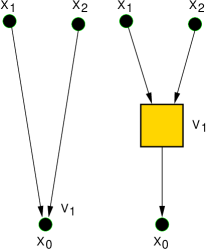
Figure 1: Different representations of interactions in the graph $G$. Left: oriented graph Right: a bipartite oriented graph. $V_{1}$ is a function and $x_{i}$ are variables, $x_{0}$ is the output.

An important point concerning randomization, is that the choice of what feature to conserve and what not to conserve in the randomized counterpart is quite delicate and depends on specific considerations on the system. In the words of statistical mechanics, the typical case scenario can vary greatly with the choice of the ensemble. For instance, the network motifs shown by randomizing a network with an Erdos-Renyi random graph differ from the usual ones, for which the degree sequence is used as a topological invariant IMK+03 . In studies of biological networks, the diagonal of $B$ is normally disregarded, or assumed to have the same probability distribution as a row or a column. The use of considering it is a matter of the nature of the graph and the property under exam. For the case of transcription networks, an ensemble with structured diagonal might have some relevance. For example, for motifs discovery, sometimes one puts the diagonal to zero, and considers degree-conserving randomizations that do not involve the diagonal SMM+02 . In our earlier work on transcription networks, we have considered the autoregulators as a structured diagonal LJB05 . We will show, for our model graph ensemble, that this leads to considerably different results for the feedback. There are other biological examples where a structured adjacency matrix emerges naturally. The simplest example are mixed interaction graphs. For instance, one can consider a composition of a transcription network with a protein-interaction network (which is a non directed graph) and pose the question of evaluating the feedback on a global scale compared to randomized counterparts.

Leaf-removal algorithms.

A straightforward way to measure the amount of feedback in a graph is to count cycles. However, this is in general computationally as costly as enumerating all the paths. For this reason, it is desirable to use algorithms and order parameters that allow a quicker evaluation. To this aim, we describe three variants of a decimation algorithm, termed “leaf-removal”, that is able to remove the tree-like parts of the graph, leaving the components with feedback. We define a leaf as a variable having only incoming links, and a “free” variable, or a root, a variable having only outgoing links (Fig 2). $\gamma$ is a measure for the fraction of regulated variables, as opposed to external variables which only enter functions as inputs. The three variants of the leaf-removal iteratively remove links and nodes from the graph, using the following prescriptions (Fig 2).

1. LRa. Remove leaves and their incoming links.

2. LRb. As above. Additionally, remove incoming links of nodes whose incoming links are all connected to roots, which are also removed.

3. LRc. As LRa. Additionally, remove all the incoming links (together with their associated nodes) of nodes whose incoming links are connected to at least one root.

This is an iterative nonlinear procedure, where more variables may disappear in a single move. LRc works naturally on directed and undirected bipartite graphs. In fact, viewing the system as a bipartite graph, one can verify that LRc is equivalent to removing all the functions connected to a single node, ignoring directionality. Instead, LRa and LRb are thought for a directed graph, such as the ones we consider here.

There are two possible outcomes for the leaf-removal. Removing the whole graph, or stopping at a core subgraph that contains cycles. The core is composed of $N_{C}$ genes and $M_{C}$ functions. We want to use these as order parameters for the feedback. Equivalently, we can use $\Delta_{C}=\frac{N_{C}-M_{C}}{N}$ and $\gamma_{C}=M_{C}/N_{C}$. The difference between LRa and LRb is that LRb is able to remove tree-like parts of the graph that are upstream of a simple cycle. LRc is also able to do this. On the other hand, LRc might break some of these cycles because it disregards the orientations of the edges (Fig. 2). LRc cannot break “complex” cycles, defined as cycles where each node is connected to at least two functions.

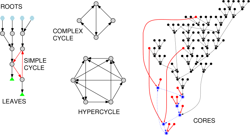
Figure 2: Left: example of roots (free variables) and leaves for the leaf-removal algorithm. This graph contains a simple cycle (in red), which is not removed by LRa and LRb, but is removed by LRc. Middle: examples of a complex cycle and a hypercycle. A complex cycle (top) is not removed by LRc, but does not belong to the kernel of of $A^{t}$. A hypercycle (bottom) is an element of the kernel of $A^{t}$, because each variable appears in an even number of functions. Right: example of cores for the different leaf-removal variants, applied on the same initial graph. The image refers to a random graph with $p=3$, $\gamma=0.5$, $N=600$. The cores are represented as a directed graph, and superimposed. The LRa core (whole figure) contains feedback loops and tree-like regions (black) upstream of the loops. The LRb core (red) does not contain the treelike parts, but all the feedback is preserved. The LRc core is empty, as this algorithm is able to break simple cycles connected to single free variables. The cycle of the original graph is indicated by circled nodes and dashed edges (blue).

Connections with Random Systems in GF2 and Adjacency Matrix Algebra.

To investigate the feedback properties of the graph, one can also consider the following linear system in the Galois field $\mathrm{GF2}$ (the set $\{0,1\}$ with the conventional operations of product, and sum modulo 2).

$$Ax=v\ \ .$$ (1)

Here, $v$ is a random vector of $\mathrm{GF2}^{M}$, that represents the functions, and $A=B+I_{MN}$, where $I_{MN}$ is the truncated $M\times N$ identity matrix, and the sums are in $\mathrm{GF2}$. In other words, we imagine that each output variable is subject to a random XOR constraint, and the idea is to use this as a probe for the feedback. Each XOR constraint, or GF2 equation corresponds to a function. In the language of statistical mechanics, the random linear system (1) maps to a p-spin model on the graph MRZ03 . The important point is that feedback translates into algebraic properties of the matrix $A$ in GF2, and in solutions of Eq. (1). A feedback loop, or a cycle, corresponds to the pair $A^{o},h^{o}$, where $A^{o}$ is a $l\times l$ submatrix of $A$, and $h^{o}$ is a $l$-component vector such as $h^{o}A^{o}=0$. Indeed, the functions and variables selected by the nonzero elements of $h^{o}$ are such that each variable appears in an even number of constraints.

We can also define a “hypercycle” as an $M$ component vector $h$ of GF2, such as the right product $hA=0$, because the functions and variables selected by the ones in $h$ are such that each variable appears in an even number of functions. Graphically, a hypercycle is a connected cluster made of functions that share an even number of nodes (Fig. 2). From the algebraic point of view, it is an element of the kernel of $A^{t}$, and is then connected to the solvability of Eq. (1). This consideration enables to evaluate the average number $\overline{\cal N}$ of solutions of Eq. 1. Perhaps surprisingly, one can prove that $\overline{\cal N}=2^{N-M}$ under very general conditions. However, this average ceases to be significant when the hypercycles become extensive (i.e., the number of nodes they involve has order $N$), as the fluctuations become dominant. This is discussed in detail in Appendix A.1. The exact threshold for $\gamma$ where hypercycles become extensive is a phase transition in the thermodynamic limit $N\to\infty,\ \ M\to\infty$ at constant $\gamma$. Precisely, it is called the SAT-UNSAT transition for Eq. (1) MPZ02 . The UNSAT threshold depends on the graph ensemble, and has been determined in some cases Kol98 . In some instances, there may exist also an intermediate “HARD-SAT” or glassy phase, where $2^{N-M}$ solutions exists, but they belong to basins of attractions whose distance from each other MPZ02 is order $N$. For a p-spin problem on a graph, this glassy phase corresponds to the presence of complex cycles MRZ03 .

Structured diagonal.

As a hypercycle is a particular realization of a complex cycle, it is easy to understand how the core of a leaf-removal algorithm will in general (but not always) contain hypercycles: none of the algorithms is able to break these structures. This is shown in Appendix A.2, which discusses the relation of the leaf-removal “moves” with operations on the rows and columns of $A$, related to the solution of Eq. (1). As explained there, for a directed graph, the extensive hypercycle, or UNSAT region may exist only at $\gamma=1$. In the case where the diagonal is structured, the situation is quite different, and the hypercycle phase can appear for $\gamma<1$ LJB05 ; CLP+06 . The above consideration justifies from an abstract standpoint the intermediate situations, with a fixed fraction of ones on the diagonal of $A$. In considering this ensemble of matrices with structured diagonal, we can introduce an additional parameter $\chi$, that represents the fraction of ones on the diagonal of $A$. It is important to note that the introduction of a structured diagonal in $A$ changes the adjacency matrix, and thus the graph ensemble. This change can have different interpretations. Rather than focusing on a particular one, the objective here is to show on an abstract standpoint how the phase behavior of Eq. (1) is perturbed by $\chi$.

III Regimes of Feedback

In this section, we discuss numerical and analytical results for the leaf-removal algorithms that support the general considerations above. We considered mainly the ensemble of graphs with fixed indegree $p$ and Poisson-distributed outdegree $k$, $p(k)=\frac{(p\gamma)^{k}}{k!}e^{-p\gamma}$. The diagonals are thrown with independent probability, to ensure that the average fraction of ones is $\chi\in[0,1]$. The choice of a structured diagonal does not perturb the marginal probability distributions of columns or rows. One can connect $\chi$ to the notion of “orientability”. If $M>N$, it is impossible to orient a graph assigning one single output per function. On the other hand, a graph with a structured diagonal can be seen as a partially oriented one, where some directed constraints coexist with some undirected ones. In this interpretation $\chi=1$ is the simple directed graph with no self-links. The case $\chi=0$ can be seen as a totally undirected graph, a similar ensemble to that used in MRZ03 .

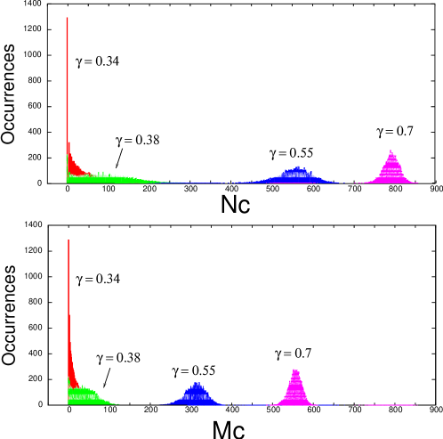
Figure 3: Histogram of the core dimensions $N_{C}$ and $M_{C}$ as a function of $\gamma$ for LRb. The data refer to $10^{4}$ random networks with $p=3$ and initial size $N=1000$. For low $\gamma$, the cores are clustered towards the empty graph. At $\gamma\simeq 0.38$ the core distribution becomes wide. Successively, the mean values grow and the histogram acquires again a sharp single peak at increasing $M_{C},N_{C}$. This is reminiscent of a second order phase transition. For LRc, this transition is much sharper (first order), and marks the onset of complexity in the core solutions $\gamma_{d}^{c}$.

We start with the totally orientable case $\chi=1$. For each value of $\gamma$, at fixed network size $N$, one can generate randomized graphs and evaluate their cores numerically. This procedure is exemplified in Fig. 3 for the case of LRb. The figure shows a transition to a regime where the core is nonempty and all the graphs are sharply distributed around the average core size. Equivalently, one can evaluate the core order parameter $\Delta_{C}$, which vanishes when the core is empty or $M_{C}=N_{C}$. The same order parameter is negative when $M_{C}>N_{C}$. Each LR has two critical values. The first, $\gamma_{d}^{x}$, is associated to the emergence of a nonempty (extensive) core. The second $\gamma_{s}^{x}$, to the condition $N_{C}<M_{C}$. Based on our results, $\gamma_{s}$ is always the same for all three leaf-removals, and corresponds to the onset of the UNSAT phase of extensive hypercycles. From simulations and analytical work, $\gamma_{s}=1$. $\gamma_{d}^{x}$, instead, depends on the ability to remove parts of the graph of the different algorithms.

As we have seen, LRa can remove less than LRb, because the latter is able to deal with the tree-like parts of the graph that lay upstream of the loops. Also, LRb can remove less than LRc, because LRc can break feedback loops if they are connected to a single free variable. Thus, one can expect $\gamma_{d}^{a}<\gamma_{d}^{b}<\gamma_{d}^{c}$. This is indeed our observation (Fig. 4).

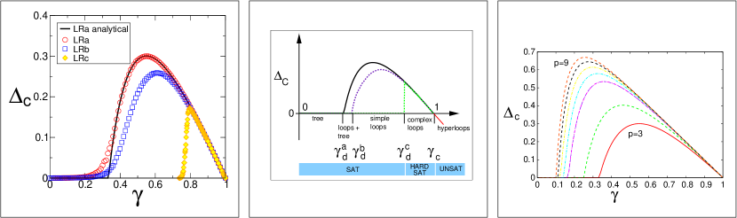
Figure 4: Left: $\Delta_{C}(\gamma)$ for $\chi=1$, $p=3$. The solid line corresponds to the analytical calculation (Appendix A.3). The symbols are numerical results for $10^{3}$ realizations of graphs with $N=1000$. $\gamma_{d}^{a}<\gamma_{d}^{b}<\gamma_{d}^{c}$ mark the transition to an extensive core for the three leaf-removal algorithms. $\gamma_{s}=1$ for all three algorithms to the point where $\Delta_{C}$ becomes negative. Middle: A scheme of the resulting phase diagram. Right: Analytical ($N\to\infty$) values of the order parameter $\Delta_{C}$ for the LRa algorithm, $\chi=1$ and different values of $p$. The order parameter deviates from zero at the threshold $\gamma_{d}^{a}=1/p$, and crosses again at $\gamma_{c}=1$. The calculation is described in Appendix A.3.

Based on these results, we can distinguish the following five regimes of feedback: (1) all cores are empty, (2) only the LRa core is nonempty, (3) both the LRa and the LRb core are nonempty, (4) all the cores are nonempty with $N_{C}>M_{C}$, (5) all the cores have $N_{C}<M_{C}$. These last two regimes can be seen as thermodynamic phases connected with the SAT-UNSAT transition of the associated linear system.

1. There are no feedback loops in the typical case.

2. Feedback loops emerge, that form a core having an extensive treelike component upstream. The cycles are intensive (i.e. the core contains a number of nodes negligible with respect to N, or $o(N)$), but the tree upstream becomes extensive ($O(N)$). Analytically, one can compute that $\gamma_{d}^{a}$ corresponds to the percolation-like threshold $1/p$ (see Appendix A.3 and Fig. 4). Intuitively, as soon as the graph percolates, even in the presence of a small region containing cycles, the tree upstream of the feedback loops can span an extensive part of the graph.

3. There is an extensive core of simple loops. LRb erases the tree upstream of the feedback loops, thus it can only have its threshold when the region of cycles itself becomes extensive. So far, we have not been able to compute the threshold $\gamma_{d}^{b}$ analytically. However, our simulations indicate that it lies higher than $\gamma_{d}^{a}$ (Fig. 4).

4. HARD-SAT phase. Intensive hypercycles, and extensive complex cycles form the core, where each variable appears in 2 or more functions. This gives a clustered structure to the space of solutions in the corresponding random linear system. $\Delta_{C}$ is proportional to the complexity $\Sigma$ of the space of solutions, defined by the relation $\log\mathcal{N}\sim N(\Sigma+S)$. Here $S$, the entropy, measures the width of each cluster, while $\Sigma$ counts the number of clusters.

5. UNSAT phase. The hypercycles become extensive. The threshold $\gamma_{s}=1$ can be compute analytically (see Appendix A.3, and Fig. 4)

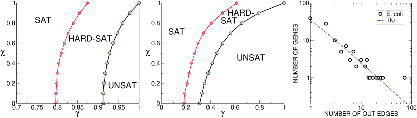
Figure 5: Left: Phase diagram for $p=3$ and structured diagonals (varying $\chi$). There are quantitative changes with respect to $\chi=1$. Middle: Phase diagram for scale-free distribution of the outdegree $k$. $\gamma_{d}^{c}$ and $\gamma_{s}$ move with the same trend and undergo a notable quantitative drift with increasing $\chi$. Right: The exponent for the outdegree distribution is a fit from data on the transcription network of E. coli SMM+02 .

Considering now ensembles with a structured diagonal, one can carry the same analysis at fixed values of $\gamma$ and $\chi$. As we discussed above, LRc is not sensitive to graph orientation, and graphs with a structured diagonal can be seen as partially oriented ones. Thus, the simplest choice is to forget the other variants of the algorithms and focus on LRc. At fixed $\chi$, there are three phases SAT, HARD-SAT, and UNSAT. On the other hand, as we argued above, because of the structure of the core matrices, these regions vary with $\chi$, and a new phase diagram can be generated. The interesting result is that this ensemble can show quantitatively different thresholds, while leaving the marginal distributions for the row and column connectivity unchanged. We have addressed this question numerically, computing the thresholds $\gamma_{d}^{c}(\chi)$ and $\gamma_{s}(\chi)$. The results for the fixed $p$ ensemble are shown in Fig. 5. The value for both thresholds increases with increasing $\chi$. In particular, $\gamma_{s}(\chi)$ becomes exactly $1$ in the directed case. On the other hand, the phenomenology of the transition does not vary with $\chi$, with a discontinuous jump at the onset of a complex cycles phase, as in a first order phase transition. Thus, in the fixed $p$ ensemble, there is a marked quantitative change in the thresholds. One may wonder whether the impact is the same for ensembles of graphs where the connectivity distributions are wider. Throughout the paper we have considered only the ensemble with fixed $p$ and Poisson distributed $k$. Notably, the effect of a structure diagonal becomes larger for scale-free distributions of $k$. This is illustrated in Fig. 5, where we show the phase diagram for a power-law distribution for $k$ with exponent $1.22$ fitted from data from E. coli SMM+02 , and independently thrown columns for $A$. In this case, the influence of the diagonal can bring the hypercycle threshold $\gamma_{c}$ down by a factor of three.

IV Discussion and Conclusions

We presented a theoretical study focused on the evaluation of feedback and the typical behavior of graphs taken from a random ensemble. The study focuses specifically on the ensemble of directed graphs with fixed indegree and Poisson outdegree. On the other hand, it is inspired by examples of biological graphs. Detecting feedback in large biological graphs and their randomized counterparts is important to understand their functioning. The use of our technique is that it allows for a quick evaluation and, more importantly, it provides some quantitative large-scale observables that can be used to measure the weight and the complexity of feedback loops. In order to do this, we introduce different variants of the leaf-removal algorithm, which naturally carry the definition of simple order parameters, depending on the properties of the core. We showed how the three algorithms relate to graph properties, algebraic operations on the adjacency matrix, and to solutions of the associated linear systems of equations in GF2. This analysis naturally leads to the abstract introduction of structured random graphs that conserve the number of entries in the diagonal of the adjacency matrix, which might be relevant in some biological situation.

Our two main results are the following. First, a phase diagram of different regimes of feedback depending on the fraction of free variables for an oriented graph. It shows a quite rich behavior of phase transitions that are interesting from the statistical physics viewpoint. These include the thresholds observed in diluted spin systems and XOR-like satisfiability problems. As already observed in MRZ03 , the onset of the complex phase is deep in the region where cycles exist and they involve a subgraph of the order of the graph size. On the other hand, the less intricate feedback regimes of intensive simple cycles connected to extensive trees, and of extensive simple cycles, might be relevant to characterize the dynamics in biological instances. The leaf-removal algorithms enable to analyze these different forms of feedback, that can be “weaker” than the complex cycles and hypercycles that are relevant for the associated GF2 problem. The second result is that the introduction of a structured diagonal, which can be interpreted as a partial orientation in the graph, has some influence on the thresholds. This is particularly true in presence of scale-free degree distribution, where we showed a phase diagram inspired by the connectivity in the E. coli transcription network SMM+02 . The algorithms described here can be readily applied to biological data sets and their randomized counterparts. We are currently addressing this question in relation with the Darwinian evolution of some transcription and mixed transcription- and protein-interaction graphs. Finally, while this analysis is loosely inspired to graphs related to gene regulation, the need to evaluate the feedback arises in different contexts, where the tools described here could prove useful.

Appendix A Appendix

A.1 Solutions of the Random System in GF2

Evaluating the average number of solutions of Eq. 1 for large $N$ at constant $\gamma$ gives information in the feedback of the associated graph. We denote the kernel of a matrix by $K$, its range by $R$, and their dimensions by $\kappa$ and $\rho$ respectively. If the probability measure for $v$ is flat, the average number of solutions for fixed $A$ is the probability that $v\in R(A)$, i.e.

$$\mathrm{prob}(v\in R(A))=\frac{2^{\rho(A)}}{2^{M}}=2^{-\kappa(A^{t})}\ ,$$

times the number of elements in $K(A)$ (i.e. $2^{K(A)}$. The average number of solutions is thus

$$\overline{\cal N}=\langle 2^{-\kappa(A^{t})}2^{\kappa(A)}\rangle_{A}=2^{N-M}\ \ ,$$ (2)

where we have used the relations $\rho(A)+\kappa(A)=N$, $\rho(A^{t})+\kappa(A^{t})=M$, and $\rho(A)=\rho(A^{t})$. Moreover, with the same reasoning, the fluctuations in the number of solutions are

$$\overline{{\cal N}^{2}}=(\overline{\cal N})^{2}\langle 2^{\kappa(A^{t})}\rangle_{A}\ ,$$

meaning that when the average $\langle 2^{\kappa(A^{t})}\rangle_{A}$ is $O(1)$, an average number of solutions $\overline{\cal N}=2^{N-M}$ are typically found, while this is not the case if $\langle 2^{\kappa(A^{t})}\rangle_{A}$ is an extensive quantity. In fact, when this “selfaveraging” property breaks down, typically no solutions are found, because $\overline{\cal N}$ is supported only by the multiplicity of very rare $v\in R(A)$. This connects the solvability of the system to the topology of the hypercycles.

There are phase transitions between the two above regimes, tuned by the order parameter $\gamma$. The standard approach is to take the thermodynamic limit $N\to\infty,\ \ M\to\infty$ at constant $\gamma$. These transitions depend on the ensemble of graphs considered Kol98 .

A.2 Adjacency Matrix and Leaf-removal.

Let us try to visualize the leaf-removal procedure, for instance LRc, on a generic adjacency matrix. Consider a general Boolean matrix $A$ $M\times N$, and apply LRc. Each time we find a leaf, we assign it and its corresponding constraint a progressive number, and we use that number as a label for the rows. With these permutations, we construct a hierarchy for the leaves, as the leaves of layer $a$ cannot appear in the clauses of layer $b\geq a$. In the tree-like case, reordering the lines of $A$, we obtain

$$\left(\begin{array}[]{c||c|c|c|c|c||c|c}\mathrm{layer}&N&...&...&...&...&N-M&1\\ \hline\cr(1)&I&...&...&...&...&...&...\\ (2)&0&I&...&...&...&...&...\\ (...)&0&0&...&...&...&...&...\\ (m-1)&0&..&0&I&...&...&...\\ (m)&0&0&..&0&I&...&...\\ \end{array}\right)$$

where $(1)$ is the set of first layer leaves, $(2)$ the second, etc. The last $N-M$ entries of each row correspond to free variables. We have thus obtained a triangulation of $A$, where the diagonal is made of blocks (the layers) of identity matrices.

In the presence of a core, the triangulation can be carried only until a the core is reached, and the the matrix can be rearranged to show the core in the lower right corner. If the core has hypercycles, in the UNSAT phase, the matrix structure is

$$\left(\begin{array}[]{c||c|c|c|c||c}\mathrm{layer}&N...&...&...&...&N_{c}\leftarrow\rightarrow 1\\ \hline\cr(M)&1!&...&....&...&...\\ (..)&0&1!&...&...&...\\ (...)&0&0&1!&...&...\\ \hline\cr(M_{c})&0&..&0&0!&\mathrm{core}\\ (..)&0&..&0&0&``\\ (1)&0&..&0&0&``\\ \end{array}\right)$$

Here, $M_{C}>N_{C}$, so typically it will not possible to find solutions to the core linear system on GF2, or the core does not contain sufficient free variables. When the ensemble for $A$ is specified, one has to apply this procedure to all the realizations. Naturally, the outcome depends on the matrix ensemble. It also depends in general on the variant of leaf-removal that one applies.

Structured diagonal.

Focusing on the diagonal of $A$, we note that in presence of hypercycles, one has necessarily to have some zeros in the $M\times M$ submatrix of $A$ to realize the condition $N_{c}<M_{c}$. This can be seen in the sketch above, where the diagonal elements are followed by an exclamation mark. In particular, the diagonal contains an extensive number of ones. Thus, following the above argument, it is easy to realize that $M_{c}\leq N_{c}$, and the hypercycle phase may exists only marginally at $\gamma=1$. For our main choice of ensemble, this is the case, as each variable can have only one input, so each constraint can always be labeled by the name of its output variable, which will appear as a one in the diagonal of $A$. In the case where the diagonal contains an extensive number of zeros, the situation is quite different, and the hypercycle phase can appear for $\gamma<1$ LJB05 ; CLP+06 .

A.3 Analytical results for LRa

We present here the analytical calculation for LRa. If $f_{k}$ is the probability to have $k$ outputs, LRa defines a dynamics for it, associated by the cancellations of leaves at each time step. For every time $t$, one can write

$$\begin{array}[]{l}N=N\>\sum f_{k}(t)\ ;\vspace{0.1cm}\\ N(t)=N\>\sum_{k\geq 1}f_{k}(t)=N\>(1-f_{0}(t))\ ;\\ \vspace{0.1cm}M(t)\>p=N\>\sum kf_{k}(t)\ .\end{array}$$

The fraction of nonempty columns is given by the probability $1-f_{0}(t)$. Writing the increments as, $\Delta N_{k}=N\>\Delta f_{k}=N\>\frac{\partial f_{k}}{\partial t}\Delta t$, one can choose $\Delta t=\frac{1}{M}$, $t\in[0:1]$, and obtain intensive equations of the kind $\frac{\partial f_{k}}{\partial t}=I(t)_{k,h,f_{h}(t)}\ ,$ where $I$ is the matrix that represents the flux generated by a move Wei02 .

We now separate $A$ in the blocks $S$ and $T$ of constrained and free variables respectively, writing $A=[S|T]$. The variables that appear in $T$ have an outgoing edge but no incoming ones. $S$ has $\gamma\>N$ columns, while $T$ has $(1-\gamma)\>N$ columns. All the rows of $A$ have $p$ ones. The distribution for the ones appearing in the columns, i.e. for the outdegree $k$, is Poisson for both $S$ and $T$, $f_{k}(0)=\frac{\lambda^{k}}{k!}e^{-\lambda}$, with $\lambda(0)=p\gamma$. We impose $s_{i,i}=1$. The lines of $A$ contain on average $p\gamma$ elements in $S$ and $(1-\gamma)p$ elements in $T$, thus after one move there are on average $p\gamma+1$ elements in $S$. Defining $p^{\prime}=p\>\gamma+1$. The flux equations can be written as

$$\begin{array}[]{l}\frac{df^{S}_{k}}{dt}=\frac{p^{\prime}-1}{<k>^{S}(t)-1}[kf^{S}_{k+1}-(k-1)f^{S}_{k}];\quad\mathrm{for~{}}k>1\vspace{0.1cm}\\ \frac{df^{S}_{1}}{dt}=-1+\frac{p^{\prime}-1}{<k>^{S}(t)-1}[f^{S}_{2}]\ \ ,\\ \vspace{0.1cm}\frac{df^{S}_{0}}{dt}=1\ \ ,\end{array}$$

where $<k>(t)=\sum kf_{k}(t)$. Summing the above equations, one obtains the evolution equation for the normalization factor $m^{S}:=\sum p^{c}_{k}=<k>^{S}-1$.

$$\frac{dm^{S}}{dt}=-\frac{p^{\prime}-1}{m^{S}(t)-1}\sum(k-1)f^{S}_{k}=-p\gamma$$

With initial condition $m^{S}(0)=\lambda(0)=p\gamma$, the solution is $m^{S}(t)=p\gamma\>(1-t)$. $m^{S}(t)$ can then be identified with $\lambda(t)$ appearing in the (Poisson) distribution $f_{k}(t)$. $-\frac{\frac{d\lambda(t)}{dt}}{\lambda(t)}=\frac{p^{\prime}-1}{m^{S}(t)}=\frac{p\gamma}{p\gamma}\>\frac{1}{1-t}$, from which $\frac{\lambda(t)}{\lambda(0)}=[1-t]$. Thus, for $k>1$,

$$f^{S}_{k}=e^{\lambda(t)}\>\frac{\lambda(t)^{k-1}}{(k-1)!}\ \ .$$

For $k=1$, one can then write $\frac{\partial}{\partial t}f^{S}_{1}=-1-\frac{\frac{d\lambda}{dt}}{\lambda}\>(\lambda e^{-\lambda})$, so that

$$f_{1}^{S}(t)=-t+e^{\lambda(t)}=-t+e^{p\gamma(t-1)}\ \ .$$

The stop time $t^{*}$ of the algorithm is then a solution of the equation $t^{*}=e^{p\gamma(t^{*}-1)}$. This last equation implies that if $p\gamma<1$ the lowest solution for the stop-time is $t^{*}=1$, or, in other words, all the graph is removed. On the other hand, when $p\gamma>1$, there is a finite stop time $t^{*}<1$, and thus a core. This determines the critical value $\gamma_{d}^{a}=1/p$. The size of the portion of the core matrix contained in $S$ is given by $M^{S}_{stop}=N^{S}_{stop}=\gamma N\>(1-t^{*})$.

In order to evaluate the full core matrix and the order parameters, the same analysis has to be carried out for the matrix of the free variables, $T$. In this case, one has $p_{k}^{T}=k\frac{f^{T}_{k}}{m^{T}(t)}$, where $m^{T}(t)=\sum kf_{k}^{T}$. Again,

$$\Delta N^{T}=N(1-\gamma)\frac{\partial}{\partial t}f_{k}^{T}\Delta t=\frac{1-\gamma}{\gamma}\frac{\partial}{\partial t}f_{k}^{T}\ ,$$

and the flux equations are

$$\begin{array}[]{l}\frac{1-\gamma}{\gamma}\frac{\partial}{\partial t}f_{0}^{T}=\frac{p(1-\gamma)}{m^{T}(t)}f_{1}^{T}\ \ ,\vspace{0.1cm}\\ \frac{1-\gamma}{\gamma}\frac{\partial}{\partial t}f_{1}^{T}=\frac{p(1-\gamma)}{m^{T}(t)}[2f_{2}^{T}-f_{1}^{T}]\ \ ,\vspace{0.1cm}\\ \frac{1-\gamma}{\gamma}\frac{\partial}{\partial t}f_{k}^{T}=\frac{p(1-\gamma)}{m^{T}(t)}[(k+1)f_{k+1}^{T}-kf_{k}^{T}].\end{array}$$

The last equation can be rewritten as $\frac{\partial}{\partial t}f_{k}^{T}=\frac{p\gamma}{m^{T}(t)}[(k+1)f_{k+1}^{T}-kf_{k}^{T}]$. As above, summation yields the evolution of the normalization constant $\frac{\partial}{\partial t}m^{T}(t)=-p\gamma$.

Thus, $\frac{\frac{\partial}{\partial t}\lambda(t)^{T}}{\lambda^{T}}=\frac{p\gamma}{m^{T}(0)-p\gamma t}$, which gives

$$\frac{\lambda(t)^{T}}{\lambda^{T}(0)}=\frac{m^{T}(0)-p\gamma t}{m^{T}(0)}\ \ ,$$

$$f^{T}_{0}(\lambda)=e^{-\lambda}\ \ .$$

In conclusion, the stop time $t^{*}$ is a function of $(p\gamma)$, determined by the relation $t^{*}=e^{p\gamma(t^{*}-1)}$. The transition value to an extensive core is then given by $\gamma_{d}^{a}=1/p$. The core dimensions can be written as $M^{S}_{C}=N\>\gamma(1-t^{*})$, and $N^{T}_{C}=(1-\gamma)(1-f_{0}^{T})=(1-\gamma)(1-t^{*})$. This last quantity gives the core order parameter $\Delta_{C}=(1-\gamma)(1-t^{*})$. $\Delta_{C}$ is zero for $\gamma<\gamma_{d}^{a}$, and becomes nonzero at this critical value, in a continuous, non-differentiable way (with an infinite jump). The other threshold is easily calculated, as, for any finite $p\gamma$, $t^{*}>0$, thus $\gamma_{c}$ is given by the prefactor $1-\gamma$ in $\Delta_{C}$ crossing zero and becoming negative: $\gamma_{c}=1$.

References

- (1) Uetz, P., Finley, Jr, R.: From protein networks to biological systems. FEBS Lett 579(8) (2005) 1821–7
- (2) Babu, M., Luscombe, N., Aravind, L., Gerstein, M., Teichmann, S.: Structure and evolution of transcriptional regulatory networks. Curr Opin Struct Biol 14(3) (2004) 283–91
- (3) Davidson, E., Rast, J., Oliveri, P., Ransick, A., Calestani, C., Yuh, C., Minokawa, T., Amore, G., Hinman, V., Arenas-Mena, C., Otim, O., Brown, C., Livi, C., Lee, P., Revilla, R., Rust, A., Pan, Z., Schilstra, M., Clarke, P., Arnone, M., Rowen, L., Cameron, R., McClay, D., Hood, L., Bolouri, H.: A genomic regulatory network for development. Science 295(5560) (2002) 1669–78
- (4) Price, N., Reed, J., Palsson, B.: Genome-scale models of microbial cells: evaluating the consequences of constraints. Nat Rev Microbiol 2(11) (2004) 886–97
- (5) Yook, S., Oltvai, Z., Barabasi, A.: Functional and topological characterization of protein interaction networks. Proteomics 4(4) (2004) 928–42
- (6) Hurst, L., Pal, C., Lercher, M.: The evolutionary dynamics of eukaryotic gene order. Nat Rev Genet 5(4) (2004) 299–310
- (7) Kepes, F.: Periodic epi-organization of the yeast genome revealed by the distribution of promoter sites. J Mol Biol 329(5) (2003) 859–65
- (8) Teichmann, S., Babu, M.: Gene regulatory network growth by duplication. Nat Genet 36(5) (2004) 492–6
- (9) Hahn, M., Conant, G., Wagner, A.: Molecular evolution in large genetic networks: does connectivity equal constraint? J Mol Evol 58(2) (2004) 203–11
- (10) Luscombe, N., Babu, M., Yu, H., Snyder, M., Teichmann, S., Gerstein, M.: Genomic analysis of regulatory network dynamics reveals large topological changes. Nature 431(7006) (2004) 308–12
- (11) Milo, R., Itzkovitz, S., Kashtan, N., Levitt, R., Shen-Orr, S., Ayzenshtat, I., Sheffer, M., Alon, U.: Superfamilies of evolved and designed networks. Science 303(5663) (2004) 1538–42
- (12) Thomas, R.: Boolean formalization of genetic control circuits. J Theor Biol 42(3) (1973) 563–85
- (13) Lagomarsino, M., Jona, P., Bassetti, B.: Logic backbone of a transcription network. Phys Rev Lett 95(15) (2005) 158701
- (14) Correale, L., Leone, M., Pagnani, A., Weigt, M., Zecchina, R.: Core Percolation and Onset of Complexity in Boolean Networks. Phys. Rev. Lett. 96 (2006) 018101
- (15) Bauer, M., Golinelli, O.: Core percolation in random graphs: a critical phenomena analysis. Eur. Phys. J. B 24 (2001) 339–352
- (16) Mezard, M., Ricci-Tersenghi, F., Zecchina, R.: Alternative solutions to diluted p-spin models and XORSAT problems. J. Stat. Phys 505 (2003)
- (17) Levitskaya, A.A.: Systems of Random Equations over Finite Algebraic Structures. Cybernetics and System Analysis 41(1) (2005) 67
- (18) Itzkovitz, S., Milo, R., Kashtan, N., Ziv, G., Alon, U.: Subgraphs in random networks. Phys Rev E Stat Nonlin Soft Matter Phys 68(2 Pt 2) (2003) 026127
- (19) Mezard, M., Parisi, G., Zecchina, R.: Analytic and algorithmic solution of random satisfiability problems. Science 297(5582) (2002) 812–5
- (20) Kolchin, V.F.: Random Graphs. Cambridge University Press, New York (1998)
- (21) Shen-Orr, S., Milo, R., Mangan, S., Alon, U.: Network motifs in the transcriptional regulation network of Escherichia coli. Nat Genet 31(1) (2002) 64–8
- (22) Weigt, M.: Dynamics of heuristic optimization algorithms on random graphs. Eur. Phys. J. B 28 (2002) 369